Understanding coastal wetland conditions and futures by closing their hydrologic balance: the case of the Gialova lagoon, Greece - Journal ...
←
→
Page content transcription
If your browser does not render page correctly, please read the page content below
Hydrol. Earth Syst. Sci., 24, 3557–3571, 2020
https://doi.org/10.5194/hess-24-3557-2020
© Author(s) 2020. This work is distributed under
the Creative Commons Attribution 4.0 License.

Understanding coastal wetland conditions and futures by closing
their hydrologic balance: the case of the Gialova lagoon, Greece
Stefano Manzoni1,2 , Giorgos Maneas1,3 , Anna Scaini1,2 , Basil E. Psiloglou4 , Georgia Destouni1,2 , and
Steve W. Lyon1,2,5,6
1 Department    of Physical Geography, Stockholm University, 10691 Stockholm, Sweden
2 Bolin  Centre for Climate Research, Stockholm University, 10691 Stockholm, Sweden
3 Navarino Environmental Observatory, 24001, Messinia, Greece
4 Institute for Environmental Research & Sustainable Development, National Observatory of Athens, 15236, Athens, Greece
5 The Nature Conservancy, 08314 Delmont, New Jersey, USA
6 School of Environment and Natural Resources, Ohio State University, 43210 Columbus, Ohio, USA

Correspondence: Stefano Manzoni (stefano.manzoni@natgeo.su.se)

Received: 22 July 2019 – Discussion started: 19 August 2019
Revised: 27 April 2020 – Accepted: 12 June 2020 – Published: 15 July 2020

Abstract. Coastal wetlands and lagoons are under pressure        ter inputs are enhanced by restoring hydrologic connectivity
due to competing demands for freshwater resources and cli-       between the lagoon and the surrounding freshwater bodies.
matic changes, which may increase salinity and cause a           This restoration strategy would be fundamental to stabilizing
loss of ecological functions. These pressures are particularly   the current wide seasonal fluctuations in salinity and main-
high in Mediterranean regions with high evaporative demand       tain ecosystem functionality but could be challenging to im-
compared to precipitation. To manage such wetlands and           plement due to expected reductions in water availability in
maximize their provision of ecosystem services, their hydro-     the freshwater bodies supporting the lagoon.
logic balance must be quantified. However, multiple chan-
nels, diffuse surface water exchanges, and diverse groundwa-
ter pathways complicate the quantification of different water
balance components. To overcome this difficulty, we devel-       1   Introduction
oped a mass balance approach based on coupled water and
salt balance equations to estimate currently unknown water       Coastal wetlands and lagoons regulate hydrologic, sediment,
exchange fluxes through the Gialova lagoon, southwestern         and contaminant exchanges between inland water bodies and
Peloponnese, Greece. Our approach facilitates quantification     the sea; they sustain biodiverse and highly productive ecosys-
of both saline and freshwater exchange fluxes, using mea-        tems and provide important ecosystem services (Thorslund
sured precipitation, water depth and salinity, and estimated     et al., 2017; Newton et al., 2014). The maintenance of these
evaporation rates over a study period of 2 years (2016–2017).    essential functions is threatened by competing demands and
While water exchanges were dominated by evaporation and          climatic changes. Reduced freshwater inflows due to inten-
saline water inputs from the sea during the summer, precipi-     sified water use in upstream catchments, drainage efforts to
tation and freshwater inputs were more important during the      convert wetlands to agricultural areas, and construction of
winter. About 40 % and 60 % of the freshwater inputs were        infrastructure that interferes with the natural water flows are
from precipitation and lateral freshwater flows, respectively.   all causes of reduced wetland functionality from both eco-
Approximately 70 % of the outputs was due to evaporation,        logical and human perspectives (e.g., Jaramillo et al., 2018;
with the remaining 30 % being water flow from the lagoon         Newton et al., 2014). In regions with high population den-
to the sea. Under future drier and warmer conditions, salin-     sity and therefore a higher risk of wetland overexploitation,
ity in the lagoon is expected to increase, unless freshwa-       these anthropogenic changes are compounded with ongoing
                                                                 climatic trends, resulting in lower precipitation and higher

Published by Copernicus Publications on behalf of the European Geosciences Union.
3558 S. Manzoni et al.: Understanding coastal wetland conditions and futures by closing their hydrologic balance
evaporation rates. These trends are expected to continue and 2 Methods
possibly worsen as global temperatures rise.
Mediterranean lagoons in particular are under pressure due 2.1 Study area and climatic conditions
to competing demands for water resources from agriculture,
tourism, the fish industry and ecological systems relying on The Gialova lagoon is located in southwestern Messinia,
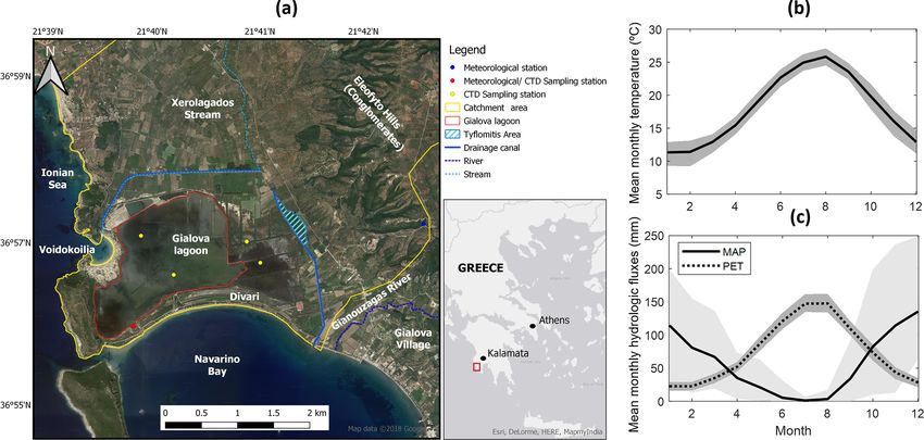
lagoons for their survival (Maneas et al., 2019; Perez-Ruzafa Greece (36.97◦ N, 21.65◦ E; Fig. 1a). The main water body
et al., 2011). While runoff is already decreasing in this region of the lagoon, on which this contribution focuses, covers
(e.g., Destouni and Prieto, 2018), climatic changes are ex- an area of a 225.5 ha; an additional 85.2 ha is covered by
pected to increase aridity by lowering the difference between surrounding wetland areas (Maneas et al., 2019). The spa-
precipitation and potential evapotranspiration by as much tial average of water depth in the main water body is ap-
as 2–4 mm d−1 on an annual basis (Gao and Giorgi, 2008; proximately 0.6 m, with a range between 0.27 and 0.77 m
Cheval et al., 2017). Therefore, coastal areas in the Mediter- (Dounas and Koutsoubas, 1996). The lagoon is delimited by
ranean region (and wetlands in particular) are regarded as sand barriers formed around 5000 yr BP (Emmanouilidis et
vulnerable to climatic changes (Klein et al., 2015; Gao and al., 2018), which separate the lagoon from Navarino Bay to
Giorgi, 2008). the south and Voidokilia Bay to the northwest. It is reason-
To study the consequences of changing hydrologic able to assume that groundwater exchanges occur through
regimes on wetlands (in terms of water quantity and quality), these relatively narrow sand barriers; in addition, a perma-
it is necessary to quantify hydrologic fluxes. This is generally nently open canal connects the Gialova lagoon to Navarino
difficult due to the complex land–water interactions in wet- Bay. The Palaiokastro hill delimits the lagoon on the west
lands, and compound interactions of land and sea with lagoon side, whereas on the north the lagoon is separated from agri-
water bodies. The lack of monitoring data for these multi- cultural areas by a canal built in 1960 to divert water from
ple pathways of water exchange makes the prediction of hy- the Xerolagados River directly to Voidokilia Bay. On the east
drologic changes challenging, requiring indirect approaches and southeast sides, wetland areas surround the main lagoon
that leverage the limited available data. To this end, overar- water body. The Tyflomitis artesian springs provide freshwa-
ching mass balance considerations and closure over a whole ter to this area, thanks to freshwater aquifers feeding them
lake or wetland system can help constrain unknown fluxes of from the east (Pantazis, 2019). Historically, the flow from
water, solutes and latent heat (Destouni et al., 2010; Jarsjo these springs was approximately ≈ 1.6×10⁶ m3 yr−1 , but un-
and Destouni, 2004; Assouline, 1993). Previous examples der current conditions it is limited to ≈ 5 × 10⁵ m3 yr−1 due
have also demonstrated the advantage of this approach for to water extraction upstream (Maneas et al., 2019). Further-
coastal lagoons (Martinez-Alvarez et al., 2011; Rodellas et more, only an unknown fraction of this flow enters the wet-
al., 2018). In this contribution, we develop this approach and lands and lagoon, through up-welling and surface freshwater
describe a minimal coupled water–salt mass balance model bodies, due to a diversion canal carrying most of the spring
to determine both freshwater and saline flux exchanges of water to Navarino Bay. On the north side, the canal draining
coastal water bodies. the Xerolagados river is currently not connected with the la-
While this approach is general, we focus its application goon, but groundwater from the alluvial plain probably con-
on the Gialova lagoon (southwestern Peloponnese, Greece), tributes freshwater to the lagoon, at least during the wet sea-
the center of a Natura2000 protected area with a long history son. However, this aquifer is prone to salt intrusion from the
of water resource management that has radically altered the Gialova lagoon during the dry season (Pantazis, 2019).
lagoon functioning (Maneas et al., 2019). This hydrologic The area is characterized by a Mediterranean climate, with
system, characterized by unquantified point and diffuse wa- mild wet winters and dry summers (Fig. 1b and c). The mean
ter exchanges between lagoon and inland freshwater bodies, annual temperature is 18 ◦ C and the mean annual precipita-
and between the lagoon and the Ionian Sea, offers an oppor- tion is 695 mm yr−1 (measured from 1956 to 2011 at the Hel-
tunity to apply the mass balance approach to estimate un- lenic National Meteorological Service’s station of Methoni,
known hydrologic fluxes. Specifically, we start by quantify- 15.6 km south of the Gialova lagoon (Hellenic National Me-
ing freshwater and saline water exchange rates over a period teorological Service, personal communication, 2019). Trends
of 2 years, to evaluate the Gialova lagoon water balance for in temperature and precipitation over the measurement pe-
the study period. Second, we use the results obtained for cur- riod are weak and not statistically significant. The mean an-
rent climatic conditions and in scenarios of altered precipi- nual potential evapotranspiration has been estimated with
tation, evaporation rate, and freshwater inputs to assess how the Thornthwaite method to be 889 mm yr−1 (Maneas et al.,
climatic changes and water management may alter the lagoon 2019). Seasonal patterns are clear in all these hydroclimatic
salinity, used here as a proxy for its ecological status. variables, with dry and hot summers and wet and mild win-
ters. Precipitation shows higher variability than temperature
and potential evapotranspiration, as indicated by larger dif-
ferences between the 5th and 95th percentiles of the monthly
values (shaded areas in Fig. 1b and c).
Hydrol. Earth Syst. Sci., 24, 3557–3571, 2020 https://doi.org/10.5194/hess-24-3557-2020S. Manzoni et al.: Understanding coastal wetland conditions and futures by closing their hydrologic balance 3559
Figure 1. (a) Map of the study area; (b) long-term mean monthly temperature; (c) long-term mean monthly precipitation (MAP) and po-
tential evapotranspiration (PET). In (b) and (c), shaded areas indicate the variability around the mean (5th and 95th percentiles). Sources
for (a): AeroGRID, CNES/Airbus DS, DigitalGlobe, Earthstar Geographics, Esri, Garmin, GeoEye, GIS user community, HERE, IGN,
© OpenStreetMap contributors 2019 (distributed under a Creative Commons BY-SA License), USDA, USGS.
2.2 Theory where A is the average surface area of the lagoon, h is the
water depth in the lagoon, P and E are the rates of precipita-
Balance equations are formulated for both water volume and tion into and evaporation from the lagoon, respectively, and
salt mass in the Gialova lagoon. The lagoon receives fresh- Qfresh and Qsalt are the exchange rates of lateral freshwa-
water inputs from precipitation and both surface water and ter and saline water fluxes into and from the lagoon (vol-
groundwater fluxes, and saline water from the Navarino and umetric flow rates normalized by the lagoon area A). This
Voidokilia bays (collectively referred to as “sea” in the fol- formulation rests on the assumption that variation and po-
lowing). Outputs include evaporation and water discharge to tential trends in water level are small, so that they do not
the sea. Salt is exchanged with the sea (input or output de- significantly alter the extent of the lagoon area, which can
pending on flow direction), and the salt exchange fluxes de- then be sufficiently well represented by the average area A
pend on both the water fluxes and the salinity of the source over the study period. This assumption is reasonable because
water body. All water exchanges, except precipitation (mea- the shoreline is mostly limited by man-made constructions
sured) and evaporation rate (modeled based on local mete- with steep walls; only at the northwest side of the lagoon is a
orological data), are regarded as unknown. For convenience, small area seasonally flooded. Assuming essentially constant
water and salt fluxes are defined as positive when entering the lagoon area, changes in volume (V = hA) can be approxi-
lagoon. Water fluxes are expressed as volume per unit area mated as A times the changes in water depth ( dV dh
dt ≈ A dt ),
of the lagoon and time (e.g., mm d−1 ) and salt mass fluxes as justifying the first equality in Eq. (1).
mass per unit area and time (e.g., g m−2 d−1 ); concentrations In Eq. (1), precipitation rate and water depth are measured,
are expressed as mass per unit volume of water (e.g., g L−1 ). while evaporation is estimated using the Penman equation,
Subscript “G” indicates the Gialova lagoon; subscript “S” in- parameterized with local meteorological data (Sect. 2.2.3).
dicates sea water. Symbols are listed and defined in Table 1. The two remaining water fluxes, Qfresh and Qsalt , are un-
known and therefore solved for. A second equation is then
2.2.1 Water balance equation necessary to obtain the two unknowns at each time step; this
additional equality is provided by the salt balance.
An overarching balance equation for water volume, neglect-
ing water density variations, can be formulated for the lagoon
in terms of its average water depth and the main water fluxes
that regulate it as
1 dV dh
= = P − E + Qfresh + Qsalt , (1)
A dt dt
https://doi.org/10.5194/hess-24-3557-2020 Hydrol. Earth Syst. Sci., 24, 3557–3571, 20203560 S. Manzoni et al.: Understanding coastal wetland conditions and futures by closing their hydrologic balance
Table 1. Definition of symbols used in the mass balance model and in the calculation of the evapotranspiration rate.
Symbol Description Units
Water and salt balance model (Eqs. 1–6)
A Gialova lagoon area m2
CG Salt concentration in the Gialova lagoon g L−1
CS Salt concentration in the Ionian Sea (= 38.5 g L−1 ) g L−1
E Evaporation rate mm d−1
F Salt mass exchange rate g m−2 d−1
h Gialova lagoon water depth mm
M Salt mass per unit area in the Gialova lagoon g m−2
P Precipitation rate mm d−1
Qfresh Freshwater exchange rate (including surface and groundwater) mm d−1
Qsalt Saltwater exchange rate (including surface and groundwater) mm d−1
V Water volume in the Gialova lagoon m3
Runoff model (Eq. 12)
AET Actual evapotranspiration mm yr−1
PET Potential evapotranspiration mm yr−1
R Runoff from catchments surrounding the Gialova lagoon mm yr−1
Evaporation model (Eq. 7)
cp Heat capacity of air MJ kg−1 ◦ C−1
es Saturated atmospheric vapor pressure kPa
ea Actual atmospheric vapor pressure kPa
G Heat flow in the water column MJ m−2 d−1
ra Aerodynamic resistance d m−1
Rn Net radiation MJ m−2 d−1
1 Slope of the vapor pressure saturation-temperature relation kPa ◦ C−1
γ Psychrometric constant kPa ◦ C−1
λ Latent heat of vaporization MJ kg−1
ρa Air density kg m−3
ρw Water density kg m−3
2.2.2 Salt balance equation Eq. (4), Qsalt is still unknown, whereas CG is measured and
the seawater salinity CS is assumed to be constant and equal
The balance equation for the mass of salt, expressed in terms to 38.5 g L−1 (Sect. 2.3.3). With this formulation, saline in-
of salt mass per unit area of the lagoon reads puts through runoff are neglected. While this assumption is
dM not always justified (Obrador et al., 2008), in the case of the
= F, (2) Gialova lagoon, the intense water exchanges with Navarino
dt
Bay likely contribute more than inland sources to the salt
where M is the salt mass per unit area (in g m−2 ) and F is the
budget.
salt exchange rate per unit area (in g m−2 d−1 ). Salt inputs
Summarizing, we have now two equations in two un-
via precipitation and atmospheric deposition are neglected
knowns (i.e., Qfresh and Qsalt ):
(as in Obrador et al., 2008, for example). Following the above
notations for water variables and assuming that waterborne dh
salt transport is purely advective, the total salt mass and salt = P − E + Qfresh + Qsalt , (5)
dt
exchange rate can be calculated as d (CG h)
CG Qsalt Qsalt < 0
= . (6)
M = CG h, (3) dt CS Qsalt Qsalt > 0
CG Qsalt Qsalt < 0 This system of equations is solved numerically using the fi-
F= . (4)
CS Qsalt Qsalt > 0 nite difference method (Sect. 2.2.4), yielding the unknown
In Eq. (3), the salt mass is obtained as the product of salt con- freshwater and saltwater exchange rates. There are uncer-
centration (CG ) and water depth (h) in the Gialova lagoon. In tainties associated with almost all fluxes and compartments,
Hydrol. Earth Syst. Sci., 24, 3557–3571, 2020 https://doi.org/10.5194/hess-24-3557-2020S. Manzoni et al.: Understanding coastal wetland conditions and futures by closing their hydrologic balance 3561
but mathematically the problem is “closed” – that is, there Sect. 2.2.3. To proceed, Qfresh and Qsalt in Eqs. (5) and (6)
is enough information to obtain both Qfresh and Qsalt . Both must be expressed as functions of these known quantities.
mass balance equations are solved with a daily time resolu- Equation (6) allows Qsalt to be found through
tion, but the results are aggregated to the monthly scale and (
1 d(CG h)
over the whole study period. CG dt Qsalt < 0
Qsalt = 1 d(CG h) . (8)
CS dt Qsalt > 0
2.2.3 Evaporation rate
Using the chain rule of differentiation and discretizing
The evaporation rate (E, expressed in mm d−1 ) is calculated through time, we obtain
using the Penman equation, parameterized following Duan
and Bastiaanssen (2017), d (CG h) dCG dh 1CG 1h
=h + CG ≈h + CG , (9)
1000
1 ρa cp es − ea
dt dt dt 1t 1t
E= (Rn − G) + , (7)
λρw 1 + γ 1 + γ ra where 1t is the discretization time step. If h 1C G 1h
1t + CG 1t >
where all symbols are listed in Table 1 and the factor 1000 0, salt mass increases and it follows that Qsalt > 0, so that
converts units from meters per day (m d−1 ) to millimeters per the second expression in Eq. (8) is used to obtain Qsalt . In
day (mm d−1 ). contrast, if h 1C G 1h
1t + CG 1t < 0, salt mass decreases and the
To use Eq. (7) with the available data (Sect. 2.3), several first equation is used. Therefore, combining Eqs. (8) and (9),
assumptions are made. First, at the daily timescale, the con- we finally obtain
tribution of heat flow in the lagoon (G) is neglected. Second,
net radiation (Rn ) is calculated as the difference between
1
CG h 1C
1t
G
+ CG 1h
1t , h 1C G 1h
1t + CG 1t < 0
Qsalt =
1CG
. (10)
incoming shortwave plus longwave radiation, and outgoing 1
CS
1h
h 1t + CG 1t , h 1C G 1h
1t + CG 1t > 0
shortwave plus longwave radiation, of which only incoming
shortwave radiation is measured. Reflected shortwave radia- The next step requires discretizing and solving Eq. (5) to ob-
tion is estimated assuming an albedo of water equal to 0.08 tain Qfresh from the other hydrologic fluxes, changes in water
(McMahon et al., 2013). Net outgoing longwave radiation is depth, and Qsalt from Eq. (10),
estimated using an empirical relation that accounts for both dh 1h
surface temperature and atmospheric conditions that affect Qfresh = − P + E − Qsalt ≈ − P + E − Qsalt . (11)
incoming longwave radiation (Allen et al., 1998). In this rela- dt 1t
tion, increasing vapor pressure and decreasing solar radiation The two linked Eqs. (10) and (11) do not need to be cou-
(both quantities are measured at our site) decrease outgoing pled through time because changes in water depth (though
longwave radiation for a given surface temperature. Third, not water depth per se) and salt concentration in the lagoon
the aerodynamic resistance is parameterized for open-water are measured. These equations could thus be solved for each
evaporation following Shuttleworth (2012). To test this pa- time interval in sequence. Since the value of water depth h
rameterization, the ratio of equilibrium evaporation and to- varies from one time step to the next, and it is not mea-
tal evaporation was computed, resulting in a median value sured, h in Eq. (10) must be updated at each time step as
of 1.35 (first and third quartiles: 1.21 and 1.62, respectively). ht+1 = ht + 1h before being entered in the equation for the
While this median value is higher than the classical result by next time step. This requires setting the initial value of wa-
Priestley and Taylor (1972) for wet vegetated surfaces (i.e., ter depth for this recursive calculation to start. As long as
1.26), our values are well within the range estimated for wa- 1h/ h
1, this step would not be necessary, but since wa-
terbodies (Assouline et al., 2016). This result thus lends sup- ter depth fluctuations can be significant with respect to the
port to the adopted parameterization. Finally, and similar to mean depth in the shallow Gialova lagoon, this correction is
other studies using the Penman approach to estimate evapo- important.
ration rate (e.g., Rosenberry et al., 2007; Martinez-Alvarez To summarize, Eqs. (10) and (11) represent a simple algo-
et al., 2011; Rodellas et al., 2018), we assume that condi- rithm to calculate the unknown exchanges of water between
tions over the lagoon are homogeneous, and that our point the Gialova lagoon and the freshwater systems upstream and
measurements are representative. Considering the relatively the sea downstream during the measurement period. More-
small size of the lagoon, this assumption is deemed reason- over, they provide estimates of salt mass fluxes associated
able. with the saline water exchanges.
2.2.4 Numerical approach to solve the balance 2.2.5 Simulation scenarios
equations
To assess the effects of changing climatic conditions and wa-
The known quantities in Eqs. (5) and (6) include P , CG , ter resource management on salinity in the Gialova lagoon,
and changes in water depth ( dh 1h
dt ≈ 1t over a fixed, not in- we use Eqs. (5) and (6) in a forward mode – that is, to es-
finitesimal, time interval), and E is estimated as described in timate salinity variations through time based on hydrologic
https://doi.org/10.5194/hess-24-3557-2020 Hydrol. Earth Syst. Sci., 24, 3557–3571, 20203562 S. Manzoni et al.: Understanding coastal wetland conditions and futures by closing their hydrologic balance
fluxes. First, Eq. (5) is solved in discretized form to ob- P = 695 mm yr−1 and PET = 889 mm yr−1 ; see Sect. 2.1).
tain Qsalt for given P , E, 1h/1t, and Qfresh ; second, Qsalt is The obtained reduction coefficients are reported in Table 2.
inserted in Eq. (6), which is also solved in discretized form These climatic scenarios were further combined with al-
to calculate salinity CG . The first step requires estimates of tered water resource management scenarios, in which we as-
all hydrologic fluxes and the change in water storage except sumed that the lateral freshwater fluxes are either reduced
the unknown Qsalt . Measured precipitation and evaporation due to intensified water use or increased by attempts to re-
rates are modified to account for climatic changes, while the store the Gialova lagoon to its original state of a brackish
change in storage (dh/dt) is maintained from current condi- wetland (Table 2). To consider a wide range of possible man-
tions given the strong coupling of water levels in the lagoon agement outcomes, we considered freshwater flux changes
and in the sea (Sects. S1 and Fig. S1 in the Supplement). Sea varying continuously from a 50 % reduction to a 50 % in-
level rise is not considered in these scenarios. The Qfresh ob- crease with respect to the current conditions, as estimated
tained under current conditions as described in Sect. 2.2.4 is in Sect. 2.2.4. Management scenarios were implemented by
modified to account for both climatic and water management varying the daily modeled values of Qfresh , independently
changes. With these assumed P , E, Qfresh and dh/dt val- of climatic conditions (e.g., assuming that freshwater ex-
ues, Qsalt is calculated at each time step from the water bal- changes are fully controlled and not limited by water avail-
ance (Eq. 5), and salinity is then readily obtained with the ability). As was also done for the climate change scenar-
salt mass balance (Eq. 6). ios, all daily values of Qfresh were varied, including fresh-
We considered three climate change scenarios (Table 2): water losses from the lagoon, thereby imposing a control on
(C1) reduced precipitation, (C2) increased temperature (and the two-way connectivity of the lagoon with the surrounding
thus evaporation), and (C3) combined reduction in precipi- freshwater bodies.
tation and increase in temperature. All scenarios are based
on results of a regional climate model forced by global cli- 2.3 Measurements
matic conditions under high CO2 emissions (denoted as A2),
with predictions extending to the year 2100 (Gao and Giorgi,
2008). For C1, a precipitation reduction up to 30 % was con- 2.3.1 Permanent equipment
sidered (while keeping current E); for C2, evaporation was
increased up to 20 % due to a mean annual temperature in- Meteorological measurements were conducted with a
crease of 4 ◦ C (while keeping current P ); for C3, the changes Decagon Devices, Inc. system, including a relative humid-
in P and E were compounded. Moreover, to assess the ef- ity and air temperature sensor (VP4), a 2-D sonic anemome-
fects of changes in water–atmosphere exchanges in isolation, ter (DS-2), a solar radiation sensor (pyranometer), and a
the lateral freshwater fluxes were either maintained as un- rain gauge (ECRN-100), all installed in March 2016. Data
der current conditions or decreased to represent reductions were recorded using EM-50 loggers. These pieces of equip-
in runoff for drier conditions driven by climate change. ment, except for the anemometer, were located on the south-
In the simulations where lateral freshwater fluxes are de- ern shore of the lagoon; the anemometer was installed on a
creased, a reduction coefficient was applied to all daily val- concrete pillar in the middle of the lagoon (approximately
ues of freshwater exchanges (water entering and leaving the 1 km from the other sensors) to minimize interference from
lagoon). The reduction coefficients for each climate sce- vegetation and the nearby terrain. Three water quality and
nario were obtained by estimating future runoff R from depth measurement points were set up in the lagoon – one
catchments surrounding the lagoon using Budyko’s approach at the southern shore next to the meteorological station, one
(Choudhury, 1999). First, the relation between long-term ac- next to the concrete pillar, and one on a PVC pole located
tual evapotranspiration (AET) and potential evapotranspira- near the northern shore (Fig. 1a). The southern and north-
tion (PET) was parameterized following Choudhury (1999). ern measurement sites were equipped with one conductivity–
Second, long-term runoff was calculated as R = P − AET temperature–depth probe, while the central site had two
under the assumption of negligible change in water storage probes at different depths (all CTD-10). For this study, salin-
in the catchment, ity was estimated from the average value of the two cen-
tral sensors, considered as representative for the whole la-
P PET goon (Sect. S2; Fig. S2). Missing data from late 2017 and
R = P − AET = P − 1
, (12)
(P n + PETn ) n January 2018 were gap-filled using the time series from the
northern measurement site, which is well-correlated with that
where n = 1.8 (Choudhury, 1999). Assuming PET ≈ E, from the central measurement site (Fig. S3). Water depth
Eq. (12) allows R to be estimated when P and PET change variations were obtained from the northern sensor, which had
according to the climate scenarios C1–C3. Finally, reduc- no missing values and had remained at the same vertical po-
tion coefficients for the freshwater exchanges are calculated sition throughout the duration of the monitoring. The CTD-
as the ratios of R under future conditions (from Eq. 12) 10 at the southern shore was not used as it exhibited signif-
over R under current conditions (i.e., R = 167 mm yr−1 for icant tidal fluctuations in salinity due to the nearby channel
Hydrol. Earth Syst. Sci., 24, 3557–3571, 2020 https://doi.org/10.5194/hess-24-3557-2020S. Manzoni et al.: Understanding coastal wetland conditions and futures by closing their hydrologic balance 3563
Table 2. Climatic and management scenarios. Variations are indicated as percentage change compared to current conditions. In scenar-
ios C1–C3, freshwater inputs are either kept as under current conditions or decreased as a consequence of a higher potential evapotranspira-
tion / precipitation ratio (black and red curves in Figs. 6a and 7a, respectively).
Scenario Code Explanation Change in Change in Change in Source for P and E
precipitation evaporation freshwater variations
P (% of rate E (% of input Qfresh
current) current) (% of current)
Climate C0 Current 0% 0% 0% Fig. 4
(Fig. 6) conditions
C1 Reduced P 0 % to −30 % 0% 0 % to −57 % Gao and Giorgi (2008)
C2 Increased E 0% 0 % to +20 % 0 % to −21 % Gao and Giorgi (2008)
C3 Reduced P , 0 % to −30 % 0 % to +20 % 0 % to −67 % Gao and Giorgi (2008)
increased E
Management Decreased or All climatic All climatic −50 % to +50 % Fig. 4 and Gao and
and climate increased Qfresh scenarios scenarios (independent Giorgi (2008)
(Fig. 7) C0–C3 C0–C3 of P and E)
connecting the Gialova lagoon and Navarino Bay and thus gorithm first detected and removed outliers (values lower
cannot be regarded as representative for the whole lagoon. than the 10th percentile) in a moving window of 4 h. Sec-
ond, data points that caused the standard deviation in the
2.3.2 Field campaigns and areal estimates of salinity moving window to be higher than 4 times the standard de-
viation in a window without any error were also removed.
The representativeness of the salinity measurements from the Conductivity values (expressed in mS cm−1 ) were converted
central site was tested by comparing the point measurements to salt concentrations (g L−1 ) using the empirical relation,
to distributed measurements collected along the shore and CG = 0.4665EC1.0878 , where EC is the electrical conductiv-
in the lagoon during several intensive campaigns from 1995 ity at 25 ◦ C (Williams, 1986) (temperature corrections were
to 2018 (Sect. S2). The campaigns were conducted at differ- performed when logging the data).
ent times of the year to span the full range of salinities oc- Salinity in the Ionian Sea is set to a constant value of
curring in the lagoon. Distributed data from these campaigns 38.5 g L−1 . This value was obtained using monthly data from
were used to estimate areal average salinities that were com- 1 m depth for the period 2008–2012 from the measurement
pared to the point measurements described in Sect. 2.3.1. The buoy number 68 422 (Pylos) of the European Marine Ob-
comparison yielded a linear relation close to the 1 : 1 line servation and Data Network (French Research Institute for
(R 2 = 0.95) that was used to scale up the point measure- Exploitation of the Sea, 2018). The buoy was located ap-
ments to the whole lagoon area (Fig. S2). A summary of the proximately 10 km southwest of the Gialova lagoon and is
areal salinity estimates from all the measurement campaigns assumed representative of the salinity in both Navarino and
is also shown in Fig. S4 as a function of month to illustrate Voidokilia bays. Seasonal variations in salinity were minor
its seasonal cycle. (38.2 to 38.9 g L−1 ) compared to the variability of salinity
in the Gialova lagoon, thereby supporting our assumption of
2.3.3 Data processing time-invariant sea water salinity.
Meteorological data were collected with a sampling interval
of 5 min and averaged (or accumulated for rainfall and solar 3 Results
radiation) over a day. Gaps in the meteorological data record
were filled using time series from two other meteorological 3.1 Water fluxes under current conditions
stations – one located in an olive orchard 5 km from the Gi-
alova lagoon, the other located at Methoni (National Obser- The study period is characterized by typical Mediterranean
vatory of Athens, 2019). Details on the gap-filling procedure conditions, with mild and wet winters, and warm and dry
are reported in the Sect. S3. summers (Figs. 2 and 3). Even though winters receive most
Water electrical conductivity measurements included er- of the rainfall, some late summer storms were exceptionally
roneous readings (downward peaks with unreasonably low intense (140 mm between DOY 250 and 251 of 2016). This
conductivity values with respect to a well-defined upper en- precipitation regime, together with intense summer evapora-
velope). These erroneous values were removed with a two- tion rates sustained by high solar radiation and temperature
step de-spiking algorithm before daily averaging. The al- (Fig. 3d), contributes to strong seasonal variations in salin-
https://doi.org/10.5194/hess-24-3557-2020 Hydrol. Earth Syst. Sci., 24, 3557–3571, 20203564 S. Manzoni et al.: Understanding coastal wetland conditions and futures by closing their hydrologic balance
Figure 3. Time series of (a) daily total incoming shortwave radia-
tion, (b) daily mean relative humidity, (c) wind speed, and (d) cal-
Figure 2. Time series of (a) daily total precipitation, (b) daily mean culated evaporation rates (Eq. 7), further decomposed into equilib-
air and lagoon water temperatures (solid and dashed curves, respec- rium evaporation (dashed black curve) and “imposed E”; i.e., the
tively), daily air temperature range (shaded area), (c) lagoon water aerodynamic component of evaporation (shaded area).
depth (normalized by the mean depth), and (d) salinity.
those of the Ionian Sea (the Pearson correlation coefficient is
maximized with a lag of one day, r = 0.78; Fig. S1).
ity (Fig. 2d). Salinity tends to increase during the spring and Figure 4a illustrates monthly averaged hydrologic fluxes,
throughout the summer, peaking in late summer or early fall including precipitation, evaporation and changes in water
(hypersaline conditions, defined here with respect to the av- depth in the lagoon. Evaporation is generally higher than pre-
erage seawater salinity of 38.5 g L−1 ). Fall and winter fresh- cipitation, as expected in Mediterranean climates (Fig. 1).
water inputs eventually restore salinity below values typi- Variations in storage (i.e., water depth) are more dynamic
cal of the Ionian Sea. These seasonal fluctuations are con- than in the other two lagoon–atmosphere fluxes and do not
sistent with those reported in earlier studies (summarized in compensate for the negative hydrologic balance of the la-
Fig. S4) and depend on both hydroclimatic conditions (both goon. Given the necessity of water balance closure over the
intra- and interannual fluctuations in water balance) and in- lagoon, this suggests that other water exchanges via ground-
terannual changes in water management (Sect. 4.3). water and surface water play a significant role. The cou-
The seasonal pattern of salinity is punctuated by sudden pled water and salt mass balances (Eqs. 10 and 11) facili-
events in response to intense rainfall events. The most no- tate estimation of the freshwater and saline water exchanges
table event occurred on DOY 251 of 2016, leading to a rapid between the Gialova lagoon and surrounding water bodies
decrease in salinity from 35 to 22 g L−1 , with the lower lever (Fig. 4b), through closure of the lagoon hydrologic balance.
sustained over the following month and a half. High salinity The estimated fluxes are on the same order of magnitude of
is associated with high water levels (Fig. 2c), which tend to rainfall and evaporation rates, reaching monthly averages of
occur during the warmer months despite their higher evap- ±10 mm d−1 , and highly variable. Freshwater exchanges are
oration rate. Water levels vary largely as a function of tidal generally positive, indicating inputs to the lagoon, as might
fluctuations in the Ionian Sea (Sect. S1) and are weakly cor- be expected by the presence of a freshwater aquifer, as well
related to individual rainfall events or the seasonal fluctua- as diffuse and point inputs from streams and springs feed-
tions in hydroclimatic variables. Specifically, the water lev- ing the main water body of the lagoon. However, during the
els in the Gialova lagoon lag approximately one day behind sudden salinity increase on DOY 294 of 2016, the model sug-
Hydrol. Earth Syst. Sci., 24, 3557–3571, 2020 https://doi.org/10.5194/hess-24-3557-2020S. Manzoni et al.: Understanding coastal wetland conditions and futures by closing their hydrologic balance 3565
Table 3. Pearson correlation coefficients between pairs of hydro-
logic fluxes (or change in storage), as calculated with Eqs. (10)
and (11) at the daily timescale (asterisks (∗ ) indicate significant cor-
relations, p < 0.001).
dh/dt P E Qfresh Qsalt
dh/dt 1.00 0.29∗ 0.00 0.05 0.63∗
P 1.00 −0.29∗ −0.14∗ −0.05
E 1.00 0.05 0.15∗
Qfresh 1.00 −0.66∗
Qsalt 1.00
Figure 5. Water budgets over the whole study period for (a) current
conditions and (b) future conditions (scenario C3: reduced precipi-
tation and increased evaporation rate; see Table 2). Water volumes
Figure 4. (a) Mean monthly hydrologic fluxes, (b) saline and fresh are expressed as a percentage of the total volume entering or leaving
water exchange fluxes (from Eqs. 10 and 11, respectively), and the lagoon, and only the net saline water exchanges are included in
(c) salt mass fluxes. Positive (negative) fluxes indicate water inputs the budgets.
to (outputs from) the Gialova lagoon.
relation between fresh and saline water fluxes indicates that
variability in water exchanges between the lagoon and the
gests a rapid outflow of freshwater (where outflow is a nega- sea or land dominates over variability imposed by water–
tive flux). This outflow is consistent with the constraint set by atmosphere exchanges.
the salt water balance and is needed to explain the measured When considering the entire study period, precipitation
increase in salt concentration at nearly constant water level. represents ≈ 40 % of the water inputs to the lagoon, whereas
Throughout the study period, the saline fluxes often change the remaining 60 % is driven by freshwater exchanges, with
sign, indicating alternate periods during which either water a minor contribution by change in water level (Fig. 5a, left
from the Ionian Sea enters the lagoon (positive sign, gener- bar). Evaporation represents ≈ 70 % of the water outputs
ally during the summer months), or water from the lagoon from the lagoon, and the remaining 30 % is caused by saline
flows into the sea (negative sign, generally during winter and water loss from the lagoon to the Ionian Sea (Fig. 5a, right
spring). bar).
Some of the daily fluxes shown in Figs. 2 and 3 and the cal-
culated saline and fresh water exchange fluxes are correlated 3.2 Water fluxes under changed climate and water
(Table 3). Precipitation and evaporation rates are negatively management
correlated due to their seasonal cycle (Figs. 2a and 3d), and
variations in water level are positively correlated to precip- Climatic changes reducing precipitation and increasing evap-
itation rates. These correlations emerge from intrinsic pro- oration rate (scenario C3) are expected to alter the water bal-
cesses and relations among hydrologic variables that are not ance with respect to current conditions (Fig. 5b). The overall
explicitly parameterized in the present water and mass bal- lower inputs and higher evaporative losses are compensated
ance equations, whereas other correlations are expected from by lower outputs of saline water from the lagoon. Note that in
the physical balance relations expressed mathematically in Fig. 5b we assumed that freshwater inputs remained as they
Eqs. (10) and (11). In particular, saline water fluxes are are today, but without any management effort, the flows from
(strongly) positively correlated with water level variations the surface freshwater bodies would most likely decrease as
and (strongly) negatively correlated with freshwater fluxes, a result of lower precipitation and higher evapotranspiration
as implied by Eq. (11). The occurrence of the strong cor- in the catchments feeding the lagoon (Sect. 4.3). Figure 6a
https://doi.org/10.5194/hess-24-3557-2020 Hydrol. Earth Syst. Sci., 24, 3557–3571, 20203566 S. Manzoni et al.: Understanding coastal wetland conditions and futures by closing their hydrologic balance
Figure 7. Effect of changes in freshwater input on (a) the mean
Figure 6. Effect of climatic changes on (a) the mean salt concen- salt concentration in the Gialova lagoon and (b) the percentage of
tration in the Gialova lagoon and (b) the percentage of time under time under hypersaline conditions, under different climatic scenar-
hypersaline conditions. Different line styles refer to three scenarios ios (different line styles; see details in Table 2). Percentage time
for changes in evaporation rate; red lines refer to scenarios where is calculated for the two simulation years; for visual reference, the
freshwater fluxes are reduced as a result of climatic changes. Per- grey horizontal dotted lines indicate current salinity and duration of
centage time is calculated for the two simulation years; for visual hypersaline conditions in the Gialova lagoon, and the grey dotted–
reference, the grey horizontal dotted lines indicate current salinity dashed line in (a) indicates salt concentration in the Ionian Sea as
and duration of hypersaline conditions in the Gialova lagoon, and of today; current conditions are indicated by open circles.
the grey dotted–dashed line in (a) indicates salt concentration in the
Ionian Sea as of today; current conditions are indicated by open
circles.
with hydroclimatic changes (similar to those in Fig. 6a). De-
creasing precipitation alone moderately increases the time in
shows predicted changes in the mean salinity of the Gialova hypersaline conditions from the current 3 months per year.
lagoon as a function of gradual precipitation reduction on the As noted for changes in salinity (Fig. 6a), higher evaporation
abscissa, in combination with unchanged (scenario C1) or rates – especially when compounded with lower freshwater
increased evaporation rate (C3) while keeping current fresh- inputs – yield longer periods under hypersaline conditions,
water inputs (black lines). In addition, the effect of reduced potentially up to most of the year in the worst-case scenario.
freshwater inputs due to lower runoff from the surrounding Altering the management of surface freshwater also affects
catchments is considered (red lines). An increase of 10 % in salinity in the Gialova lagoon, as shown in Fig. 7a. Allowing
evaporation rate alone (as would be caused by higher tem- more (less) freshwater to flow into the lagoon leads to a de-
peratures) is predicted to increase salinity by approximately crease (increase) in salinity under any climate scenario. The
5 %. Any decrease in precipitation in combination with an in- change in salinity is nonlinearly related to changes in fresh-
creasing evaporation rate further increases salinity due to the water input, consistent with an overall salt dilution effect.
accumulation of salt from the marine sources. Salt accumu- Under current climatic conditions (dotted line in Fig. 7a), a
lates because it enters the lagoon during increases in sea wa- 50 % reduction in freshwater inflows leads to an annual mean
ter level, but it does not leave it again under decreases in sea salinity similar to that of the Ionian Sea. Under future cli-
level due to saline outflows (Fig. 5b). However, for a given matic conditions, a similar decrease in freshwater inputs in-
evaporation rate, when both precipitation and freshwater in- creases salinity in the lagoon to values that are much higher
puts are decreased, salinity increases more than when only than in the Ionian Sea. To prevent a transition to a saline la-
precipitation is decreased (compare red and black lines). goon under future climatic conditions, freshwater inputs need
The time spent under hypersaline conditions is a more use- to be increased by ≈ 25 %, 30 % or more than 50 % under the
ful ecological indicator than mean salt concentration, as it three scenarios of increased aridity (C1, C2, and C3, respec-
directly impacts the ecological actors. Figure 6b shows how tively). These percentages can be seen in Fig. 7a at the inter-
the percentage of time under hypersaline conditions varies sections between the current salt concentration (horizontal
Hydrol. Earth Syst. Sci., 24, 3557–3571, 2020 https://doi.org/10.5194/hess-24-3557-2020S. Manzoni et al.: Understanding coastal wetland conditions and futures by closing their hydrologic balance 3567
grey dotted line) and the three curves representing salt con- freshwater inputs dominate the water balance, as expected
centrations under the three climate scenarios. under a Mediterranean climate with relatively low precipita-
Similar patterns emerge in Fig. 7b for the duration of hy- tion.
persaline conditions. With lower freshwater inputs combined Moreover, for our well-mixed assumption to hold, the wa-
with climatic changes, the model predicts hypersaline condi- ter and salt balances used cannot be resolved at timescales
tions for up to 9 months per year. Only increasing freshwater shorter than the equilibration time for the lagoon, which we
inputs, in the absence of climatic changes, limits hypersaline estimate to be on the order of one day (Fig. S1). There-
conditions to about 2.5 months per year. fore, significant exchanges of water and salt occurring due
to shorter-term fluctuations in sea water level are neglected
but could be important at longer timescales. To address the
4 Discussion limitations of the well-mixed assumption and gain insights
into water exchanges at subdaily timescales, the Gialova la-
4.1 Approach limitations goon should be represented by a spatially explicit hydrody-
namic model; such models have been developed and used in
The proposed approach rests on several assumptions that other recent studies for the simulation of coastal and semi-
may affect our results and conclusions. First, this is a lumped enclosed sea conditions at various scales and under different
approach that neglects spatial variability by assuming well- hydroclimatic and/or water management scenarios (Chen et
mixed conditions vertically and laterally. This lumped ap- al., 2019; Vigouroux et al., 2019).
proach is comparable in scope to previous efforts on lakes Another source of uncertainty may be introduced by at-
and lagoons where no distributed salinity data are available tributing changes in electrical conductivity solely to salinity
(Assouline, 1993; Martinez-Alvarez et al., 2011; Obrado et changes (Williams, 1986). Other solutes can impact electrical
al., 2008; Rodellas et al., 2018). Following the well-mixed conductivity but not salinity, potentially leading to errors. For
assumption, the salinity in the central measurement point the current application, where we focus on relatively short
(averaging measurements of two probes spaced 25 cm apart time periods, there are likely minimal land cover or nutrient
vertically) is regarded as representative of average salinity load changes, which limits the variability of electrical con-
over the whole lagoon. While this might not be always the ductivity due to other constituents. Also, assuming relatively
case, especially after strong rain events causing high lo- stable flow pathway distributions in the landscape over the
calized freshwater inputs from the sluice gate connecting study period, the geochemical signature of groundwater is
the Tyflomitis diversion canal to the lagoon (Maneas et al., likely constant enough so that the main driver of changes in
2019), we have shown that temporal variability in spatial av- electrical conductivity is salinity from sea water rather than
erage salinity is well captured by the point measurements terrestrial sources.
(Fig. S2). Moreover, vertical mixing is ensured by wave mo-
tion and tidal fluctuations in this shallow water body. Ther- 4.2 The hydrologic balance of the Gialova lagoon
mal stratification is minimal at the temporal scale of this under current and future climate
study, as indicated by highly correlated water temperatures
at the two sampled depths in the central measurement point In the absence of direct flow measurements, the water bal-
(Pearson correlation coefficient r = 0.998). However, salt ance approach presented provides estimates of the major
fluxes depend on salinity levels where hydrological flows oc- hydrologic fluxes exchanged through the Gialova lagoon
cur. Thus, a lumped approach has the potential to overesti- (Fig. 4), allowing its overall water balance over the 2-year
mate salt fluxes by over-emphasizing salinity gradients. As- study period to be assessed. This water balance, expressed in
sessing the consequences of this assumption requires a de- terms of relative water partitioning among different input and
tailed hydrodynamic model of the lagoon. output fluxes (Fig. 5), can be compared to hydrologic flux es-
The water balance Eq. (1) constrains the unknown fresh- timates in other Mediterranean lagoons. Mar Menor – a much
water inputs, implying that any uncertainty in the other wa- larger lagoon in southern Spain, connected to the Mediter-
ter fluxes affects the freshwater input results. For example, ranean sea via five channels (Martinez-Alvarez et al., 2011)
a sudden increase in salinity not associated with significant – receives water mostly from marine sources (62 %), with
water level change leads to both saline water inputs into and smaller contributions from precipitation (24 %) and runoff
freshwater losses from the lagoon, in order to close both the (15 %; Martinez-Alvarez et al., 2011). In contrast – and simi-
salt and the water balance. The freshwater losses are diffi- lar to the Gialova lagoon – water inputs to the small Albufera
cult to interpret, but could be explained as a loss of relatively des Grau (Menorca, Spain) are dominated by runoff (71 %),
fresh water far from the lagoon–sea canal, which is substi- followed by precipitation (29 %), while in the long term this
tuted by more saline water from the Ionian Sea. It would be lagoon has a net outflow to the sea (Obrador et al., 2008). Al-
valuable to monitor two-way water exchanges at the sluice bufera des Grau loses more water through evaporation than
gates by regulating water exchanges from inland water bod- the Gialova lagoon (76 % vs. 60 %), and correspondingly less
ies to test this model implication. In the long term, however, through net exchanges with the sea (24 % vs. 40 %). Despite
https://doi.org/10.5194/hess-24-3557-2020 Hydrol. Earth Syst. Sci., 24, 3557–3571, 20203568 S. Manzoni et al.: Understanding coastal wetland conditions and futures by closing their hydrologic balance
these differences, our estimates based on mass balance calcu- measures (black curves in Fig. 7). It is reasonable to ex-
lations are still reasonable when compared to similar lagoons pect that the freshwater inputs will be reduced due to not
in the Mediterranean basin. only lower runoff from surrounding catchments under more
These estimates based on net water exchanges between the arid conditions (Eq. 12), but also increased water abstrac-
lagoons and the sea mask the underlying patterns of gross tions (Sect. 4.3). Using the Budyko curve to estimate changes
water exchanges. We estimate large two-way exchanges with in runoff from the catchments feeding the Gialova lagoon
the Ionian Sea, facilitated by the canal that connects the la- (Eq. 12), we found that a reduction in precipitation, an in-
goon with Navarino Bay (minimum cross section of 7 m2 ). crease in PET, and both changes together (as in Table 2),
Saline water inflows amount to 2490 mm yr−1 and outflows respectively cause runoff and thus freshwater inputs to de-
to 3200 mm yr−1 , with a net loss of water from the lagoon crease by 57 %, 21 %, and 67 % from the current level. Con-
to the sea of 710 mm yr−1 (with all flows normalized by the currently, groundwater levels are also expected to decrease,
average surface area of the lagoon). These gross water fluxes potentially causing saline intrusions around the lagoon – a
are on the same order of magnitude as those exchanged by process already ongoing at least at the end of the dry sea-
Mar Menor (gross saline water input: 5600 mm yr−1 ; gross son (Pantazis, 2019). The expected reductions in freshwater
output to the sea: 4800 mm yr−1 ; Martinez-Alvarez et al., inputs will likely worsen the lagoon conditions, increasing
2011) but are larger than those exchanged by Albufera des salinity during winter and spring more than predicted when
Grau (gross saline water input: 200 mm yr−1 ; gross output to climate does not constrain freshwater inputs.
the sea: 900 mm yr−1 ; Obrador et al., 2008). This is not sur- We have not assessed the effects of long-term changes in
prising, because the latter is connected to the sea via a nar- sea level. The water levels in the Gialova lagoon are well-
row channel regulated by a floodgate, which limits the water coupled to those in the Ionian Sea, with a time lag of one day
exchanges, compared to the large channels connecting Mar (Fig. S1). As a result of this tight connection, sea level rise
Menor to the sea. is expected to be mirrored by a rise in lagoon water level.
The seasonal pattern characterized by freshwater inputs This may alter the exchanges of saline water with Navarino
in the winter and spring and saline water inputs primarily Bay, since the low Divari sand barrier may be eroded, cre-
in the summer and autumn is similar to that observed in ating more channels that link the lagoon to the sea. Faster
other Mediterranean lagoons (Obrador et al., 2008; Stumpp exchanges with Navarino Bay imply that hypersaline condi-
et al., 2014). The estimated freshwater inputs amount to tions during the summer may be avoided, but also that the
1170 mm yr−1 , which are mainly partitioned between evapo- duration of periods with brackish water would then be short-
ration (≈ 40 %) and water losses to the Ionian Sea (≈ 60 %). ened. Resolving this question is beyond the scope of this
Currently, the main freshwater input to the lagoon is from study, but can be addressed in future studies coupling projec-
Tyflomitis stream and artesian springs. In that area east of the tions of sea level rise to possible geomorphological changes
lagoon, hydraulic gradients are steeper, allowing freshwater in the area.
aquifers to deliver water to the Tyflomitis springs (Pantazis,
2019). Flow estimates for these water sources are uncertain 4.3 Management options for salinity regulation
and currently range between 0.5 × 10⁶ and 2.0 × 10⁶ m3 yr−1
(Maneas et al., 2019), equivalent to approximately 220 to Water and land in the Peloponnese peninsula, where the Gi-
890 mm yr−1 of freshwater inputs after normalizing the flow alova lagoon is situated (Fig. 1a), have been intensively used
rates by the lagoon area. Our estimated freshwater inputs are at least for the last 6000 years, often resulting in major
higher but still reasonable, considering that part of the water changes in hydrologic functioning (Butzer, 2005; Weiberg
from Tyflomitis is diverted to Navarino Bay, but that unquan- et al., 2016). Land conversion to agriculture during periods
tified groundwater flows likely contribute freshwater to the of population growth and back to natural vegetation when
lagoon as well. pressure decreased, resulted in periods of sustained erosion,
The Mediterranean region is projected to become warmer change in soil surface properties, altered evapotranspiration
and drier (Cheval et al., 2017; Gao and Giorgi, 2008). By rates associated with varying vegetation types, and modifica-
reducing precipitation and associated runoff, and increasing tions of surface flow pathways due to construction of terraces
evaporation rates, future climatic conditions are expected to and other water-conserving systems. These alterations have
increase salinity unless freshwater inputs now diverted from likely caused variable freshwater inputs to coastal lagoons,
around the lagoon to the Ionian Sea are restored. To assess which have been compounded with long-term hydroclimatic
the consequences of these climatic changes, we first calcu- trends and geomorphological processes (Emmanouilidis et
lated how salinity responds to independent variations in pre- al., 2018). Arguably, the most intense alterations occurred af-
cipitation, evaporation, and freshwater inputs (black curves ter 1960, when the streams feeding the lagoon were diverted,
in Fig. 6). Results show – as expected – increases in salt con- and the lagoon was drained and isolated from the sea to ex-
centrations for all these hydrologic changes. Similarly, the pand agricultural areas (Maneas et al., 2019). Since 1976,
time spent under hypersaline conditions is expected to in- however, hydrologic linkages with the sea and partly with
crease with such climatic changes and without intervention the surface freshwater sources have been restored. In 1999,
Hydrol. Earth Syst. Sci., 24, 3557–3571, 2020 https://doi.org/10.5194/hess-24-3557-2020You can also read