Crustal structure of southeast Australia from teleseismic receiver functions - Solid Earth
←
→
Page content transcription
If your browser does not render page correctly, please read the page content below
Solid Earth, 12, 463–481, 2021
https://doi.org/10.5194/se-12-463-2021
© Author(s) 2021. This work is distributed under
the Creative Commons Attribution 4.0 License.

Crustal structure of southeast Australia from teleseismic
receiver functions
Mohammed Bello1,2 , David G. Cornwell1 , Nicholas Rawlinson3 , Anya M. Reading4 , and Othaniel K. Likkason2
1 Department Geology and Geophysics, University of Aberdeen, Aberdeen, UK
2 Department of Physics, Abubakar Tafawa Balewa University, Bauchi, Nigeria
3 Department of Earth Sciences, University of Cambridge, Cambridge, UK
4 School of Natural Sciences (Physics), University of Tasmania, Hobart, Australia

Correspondence: Nicholas Rawlinson (nr441@cam.ac.uk)

Received: 8 May 2020 – Discussion started: 8 July 2020
Revised: 14 January 2021 – Accepted: 15 January 2021 – Published: 24 February 2021

Abstract. In an effort to improve our understanding of the           3. stations located in the East Tasmania Terrane and east-
seismic character of the crust beneath southeast Australia              ern Bass Strait (ETT + EB) collectively indicate a crust
and how it relates to the tectonic evolution of the region, we          of uniform thickness (31–32 km), which clearly distin-
analyse teleseismic earthquakes recorded by 24 temporary                guishes it from VanDieland to the west.
and 8 permanent broadband stations using the receiver func-
tion method. Due to the proximity of the temporary stations      Moho depths are also compared with the continent-wide
to Bass Strait, only 13 of these stations yielded usable re-     AusMoho model in southeast Australia and are shown to be
ceiver functions, whereas seven permanent stations produced      largely consistent, except in regions where AusMoho has few
receiver functions for subsequent analysis. Crustal thickness,   constraints (e.g. Flinders Island). A joint interpretation of
bulk seismic velocity properties, and internal crustal struc-    the new results with ambient noise, teleseismic tomography,
ture of the southern Tasmanides – an assemblage of Palaeo-       and teleseismic shear wave splitting anisotropy helps provide
zoic accretionary orogens that occupy eastern Australia – are    new insight into the way that the crust has been shaped by
constrained by H –κ stacking and receiver function inversion,    recent events, including failed rifting during the break-up of
which point to the following:                                    Australia and Antarctica and recent intraplate volcanism.

 1. a ∼ 39.0 km thick crust; an intermediate–high Vp /Vs
    ratio (∼ 1.70–1.76), relative to ak135; and a broad
    (> 10 km) crust–mantle transition beneath the Lachlan        1    Introduction
    Fold Belt. These results are interpreted to represent
                                                                 The Phanerozoic Tasmanides (Collins and Vernon, 1994;
    magmatic underplating of mafic materials at the base
                                                                 Coney, 1995; Coney et al., 1990) comprise the eastern third
    of the crust.
                                                                 of the Australian continent and, through a process of subduc-
 2. a complex crustal structure beneath VanDieland, a puta-      tion accretion, were juxtaposed against the eastern flank of
    tive Precambrian continental fragment embedded in the        the Precambrian shield region of Australia beginning in the
    southernmost Tasmanides, that features strong variabil-      late Neoproterozoic and early Palaeozoic (Foster and Gray,
    ity in the crustal thickness (23–37 km) and Vp /Vs ratio     2000; Glen, 2005; Glen et al., 2009; Moresi et al., 2014)
    (1.65–193), the latter of which likely represents compo-     (Fig. 1). Persistent sources of debate that impede a more
    sitional variability and the presence of melt. The com-      complete understanding of the geology of the Tasmanides
    plex origins of VanDieland, which comprises multiple         include (1) the geological link between Tasmania – an island
    continental ribbons, coupled with recent failed rifting      state in southeast Australia – and mainland Australia, which
    and intraplate volcanism, likely contributes to these ob-    are separated by the waters of Bass Strait; and (2) the pres-
    servations.                                                  ence and locations of continental fragments from Rodinian

Published by Copernicus Publications on behalf of the European Geosciences Union.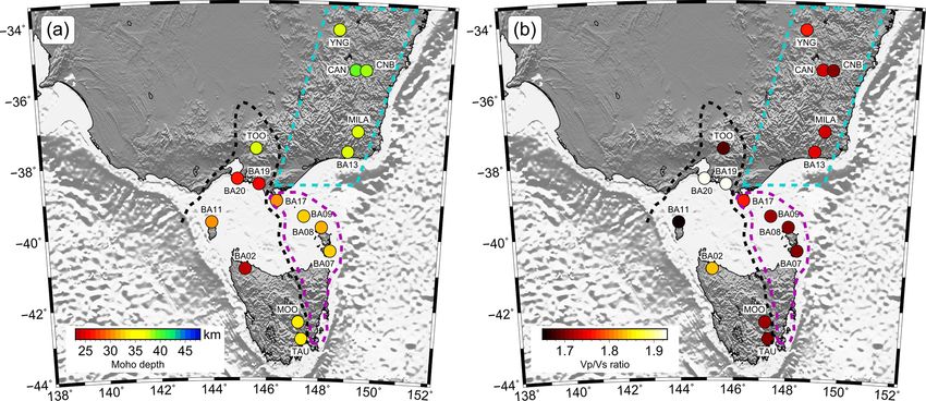
464                                                                  M. Bello et al.: Crustal structure of southeast Australia

remnants that are entrained within the accretionary orogens.       Cayley, 2011a, b; Gibson et al., 2011; Moresi et al., 2014;
Furthermore, the lateral boundaries between individual tec-        Pilia et al., 2015a, b). Particular challenges arise from mul-
tonic blocks and their crustal structure are often not well de-    tiple subduction events, multiple phases of metamorphism,
fined. To date, few constraints on crustal thickness and seis-     entrainment of exotic continental blocks, the formation of
mic velocity structure have been available for regions such        large oroclines, recent intraplate volcanism, and subsequent
as Bass Strait. Therefore, constraints on the Moho transition,     events, including the separation of Antarctica and Australia
crustal thickness, and velocity structure beneath Bass Strait      and the formation of the Tasman Sea. These challenges are
derived from receiver functions (RFs) can provide fresh in-        compounded by the presence of widespread sedimentary se-
sight into the nature and evolution of the Tasmanides.             quences that hinder direct access to basement rocks (Fig. 1).
   Previous estimates of crustal thickness and structure be-          The Tasmanides consist of four orogenic belts, namely the
neath southeastern Australia have been obtained from deep          Delamerian, Lachlan, Thomson, and New England orogens.
seismic reflection transects, wide-angle seismic data, topog-      The Delamerian Orogen – located in the south – is the oldest
raphy, and gravity anomalies (e.g. Collins, 1991; Collins et       part of the Tasmanides and has a southward extension across
al., 2003; Drummond et al., 2006; Kennett et al., 2011).           Bass Strait from Victoria into western Tasmania, where it is
Earlier RF studies in southeast Australia (Shibutani et al.,       commonly referred to as the Tyennan Orogen (Berry et al.,
1996; Clitheroe et al., 2000; Tkalčić et al., 2011; Fontaine     2008). Between about 514 and 490 Ma, the Precambrian and
et al., 2013a, b) suggested the presence of complex lateral        early Cambrian rocks that constitute the Delamerian Orogen
velocity variations in the mid-lower crust that probably re-       were subjected to a contractional orogenic event along the
flect the interaction of igneous underplating, associated thin-    margin of East Gondwana (Foden et al., 2006). Subsequently,
ning of the lithosphere, recent hotspot volcanism, and up-         the Lachlan Orogen formed in the east, which contains rocks
lift. Furthermore, the intermediate to high crustal Vp /Vs ratio   that vary in age from Ordovician to Carboniferous (Glen,
of 1.70–1.78 in this region (Fontaine et al., 2013a), relative     2005). Gray and Foster (2004) argued for a tectonic model
to ak135 continental crust where Vp /Vs is ∼1.68, may indi-        of the Lachlan Orogen that involved the interaction of a vol-
cate a mafic composition that includes mafic granulite rocks,      canic arc, oceanic microplates, and three distinct subduction
granite gneiss, and biotite gneiss. Body- and surface-wave         zones. Each subduction zone is linked to the formation of a
tomography (Fishwick and Rawlinson, 2012; Rawlinson et             distinct tectonic terrain: the Stawell–Bendigo zone, the Tab-
al., 2015) revealed P - and S-wave velocity anomalies in the       barebbera zone, and the Narooma accretionary complex. The
uppermost mantle beneath Bass Strait and the Lachlan Fold          limited rock exposure in the Tasmanides as a whole has made
Belt. Ambient noise surface wave tomography (Bodin et al.,         direct observation of the Lachlan Orogen difficult; this is at-
2012b; Young et al., 2012; Pilia et al., 2015b, 2016; Crowder      tributed to a large swath of Mesozoic–Cenozoic sedimentary
et al., 2019) of the southern Tasmanides revealed significant      cover and more recent Quaternary volcanics, which obscure
crustal complexity, but it is unable to constrain crustal thick-   a large portion of the underlying Palaeozoic terrane. How-
ness or the nature of the Moho transition.                         ever, the Lachlan Orogen contains belts of Cambrian rocks
   The goal of this paper is to provide fresh insight into the     in Victoria and New South Wales that are similar in age to
crust and Moho structure beneath the southern Tasmanides           the Delamerian Orogen (Gray and Foster, 2004).
using P -wave RFs and to explain the origin of the lateral            The presence of Precambrian outcrops in Tasmania and the
heterogeneities that are observed. This will allow us to ex-       relative lack of rocks that are similar in age in adjacent main-
plore the geological relationship between the different tec-       land Australia has led to different models which attempted to
tonic units that constitute the southern Tasmanides and to         explain the existence of Proterozoic Tasmania. For instance,
develop an improved understanding of the region’s tectonic         Li et al. (1997) suggested that western Tasmania may be the
history.                                                           remnant of a continental fragment set adrift by Rodianian
                                                                   break-up, whereas Calvert and Walter (2000) proposed that
                                                                   King Island, along with western Tasmania, rifted away from
2     Geological setting                                           the Australian craton around ∼ 600 Ma (Fig. 1). Other re-
                                                                   searchers have developed scenarios in which the island of
The Palaeozoic–Mesozoic Tasmanides of eastern Australia            Tasmania was present as a separate microcontinental block
form part of one of the most extensive accretionary orogens        that was positioned outboard of the eastern margin of Gond-
in existence and evolved from interaction between the East         wana before reattaching at the commencement of the Palaeo-
Gondwana margin and the proto-Pacific Ocean. The tectonic          zoic (Berry et al., 2008).
evolution of the Tasmanides is complex, and large-scale re-           A popular model that attempts to reconcile the geology ob-
constructions have proven difficult. This is evident from the      served in Tasmania and adjacent mainland Australia is that
variety of models that have been suggested to explain how          of Cayley (2011a). This model proposes that central Victo-
the region formed (Foster and Gray, 2000; Spaggiari et al.,        ria and western Tasmania formed a microcontinental block
2003; Teasdale et al., 2003; Spaggiari et al., 2004; Boger and     called “VanDieland” that fused with East Gondwana at the
Miller, 2004; Glen, 2005; Cawood, 2005; Glen et al., 2009;         end of the Cambrian, possibly terminating the Delamerian

Solid Earth, 12, 463–481, 2021                                                          https://doi.org/10.5194/se-12-463-2021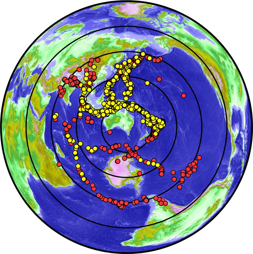
M. Bello et al.: Crustal structure of southeast Australia                                                                                 465

Figure 1. Regional map of southeastern Australia that shows key geological boundaries and the location of observed or inferred tectonic units
(modified from Bello et al., 2019a). Thick black lines delineate structural boundaries, and the thick brown dashed line traces out the boundary
of VanDieland. The following abbreviations are used in the figure: HF – Heathcote Fault; GF – Governor Fault; BF – Bootheragandra Fault;
KF – Koonenberry Fault; THZ – Torrens Hinge Zone; MA – Macquarie Arc; NVP – Newer Volcanics Province; KI – King Island in Bass
Strait; FI – Flinders Island in Bass Strait; WTT – West Tasmania Terrane; ETT – East Tasmania Terrane; AL – Arthur Lineament; TFS –
Tamar Fracture System; and RCB – Rocky Cape Block. Outcrop boundaries are sourced from Rawlinson et al. (2016).

Orogeny. VanDieland became entangled in the subduction–                   and transitional along the axis of the Tasmanides. They sug-
accretion system which built the Palaeozoic orogens that now              gested that crustal thickening of the fold belt by underplating
comprise eastern Australia (Fig. 1). Delineating Precambrian              or intrusion of mantle materials may have contributed to this
continental fragments within southeast Australia has proven               observation. Clitheroe et al. (2000) built on this earlier work
difficult, partly due to more recent sedimentary cover that ob-           by inverting RFs to map broad-scale crustal thickness and the
scures large tracts of the Tasmanides. However, if present,               Moho character across the Australian continent. They found
they likely have distinctive structural and seismic velocity              that there was generally good agreement between xenolith-
characteristics (Glen, 2013).                                             derived estimates of the Moho depth and those determined by
                                                                          RF inversion, except beneath the Lachlan Fold Belt, where
                                                                          a broad Moho transition may be present. Overall, however,
3   Previous geophysical studies                                          the RF results were consistent with those determined by
                                                                          Drummond and Collins (1986) and Collins (1991), who used
To date, a variety of geophysical methods have been em-                   seismic reflection and refraction transects to determine that
ployed to study the crustal structure of the Tasmanides.                  the Lachlan Fold Belt includes the thickest crust (∼50 km)
Shibutani et al. (1996) applied a non-linear inversion method             in eastern Australia. A more recent study by Fontaine et
to RF waveforms to constrain the shear wave velocity be-                  al. (2013a) employed H –κ stacking and non-linear RF in-
neath broadband seismic stations in eastern Australia. They               version to investigate crustal thickness, shear wave velocity
found that the Moho is relatively shallow (30–36 km depth)                structure, as well as dipping and anisotropy of the crustal lay-
and sharp within the cratonic region, and deeper (38–44 km)               ers. Their results also indicated a thick crust (∼ 48 km) and

https://doi.org/10.5194/se-12-463-2021                                                                    Solid Earth, 12, 463–481, 2021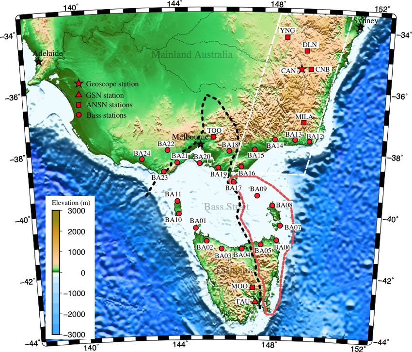
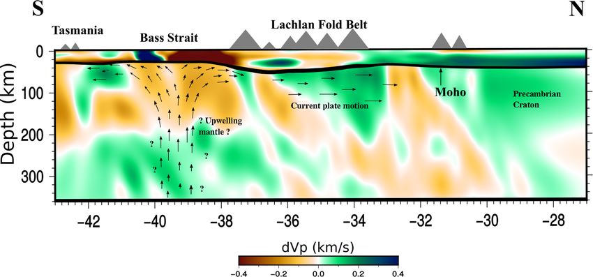
466                                                                   M. Bello et al.: Crustal structure of southeast Australia

an intermediate (2–9 km) crust–mantle transition beneath the      upper-mantle model of southeast Australia, which revealed
Lachlan Fold Belt, which could be attributed to underplating      that Bass Strait was underlain by lower velocities, consistent
beneath the crust and/or high concentrations of mafic rocks       with thinned lithosphere as a result of failed rifting during
in the mid-lower crust. Their results also showed a dipping       the break-up of Australia and Antarctica.
Moho and crustal anisotropy in the vicinity of three seismic         Active source seismic profiling has also been widely used
stations (YNG, CNB, and CAN).                                     in southeast Australia to characterize crustal velocity struc-
   Over the last decade, ambient noise tomography has             ture (e.g. Finlayson et al., 1980; Collins, 1991; Finlayson
become a popular tool for studying the structure of the           et al., 2002; Drummond et al., 2006; Glen, 2013). This has
Australian crust. Saygin and Kennett (2010) produced the          largely focused on the transition from continental to oceanic
first group velocity maps of the Australian continent from        crust at passive margins, but it has also been used to im-
Rayleigh wave group velocity dispersion in the period range       age major transition zones or faults between orogens (Glen,
from 5.0 to 12.5 s. Limited spatial resolution (∼ 2◦ × 2◦ ) in    2013) or within orogens (Cayley et al., 2011a, b), the lat-
our study region means that this model is only able to repre-     ter of which lead to the VanDieland microcontinental model.
sent the structure beneath Bass Strait as a broad, low-velocity   Rawlinson and Urvoy (2006) jointly inverted teleseismic ar-
anomaly. However, the group velocities exhibit a good cor-        rival times and active source wide-angle travel times in north-
relation with known basins and cratons. Subsequent stud-          ern Tasmania to constrain crustal velocity, Moho geometry,
ies using denser arrays covering southeast mainland Aus-          and upper-mantle velocity structure, and they found that both
tralia (Arroucau et al., 2010), southeastern Australia (Young     northeastern and northwestern Tasmania are characterized by
et al., 2013), and northern Tasmania (Young et al., 2011)         thinner (< 28 km) and higher-velocity crust compared with
show good correlations between both group and phase ve-           central Tasmania.
locity maps and sedimentary and basement terrane bound-              Potential field data have also been exploited to study the
aries. In order to account for uneven data distribution, Bodin    formation and structure of the Tasmanides. Gunn et al. (1997)
et al. (2012b) used a Bayesian transdimensional inversion         integrated potential field data (magnetic and gravity), seis-
scheme to generate group velocity maps that span the Aus-         mic reflection data, outcrop geology, and well information to
tralian continent from multi-scale ambient noise datasets.        study the crustal structure of the Australian continent. Their
However, in our study area, their model is of low resolu-         study found that the occurrence of tensional stress, oriented
tion due to the limited station coverage; hence, few details on   northeast–southwest along basement structures in the Bass
crustal structure can be inferred. Bodin et al. (2012a) subse-    Basin, is able to explain the formation of the three major sed-
quently applied Bayesian statistics to reconstruct the Moho       imentary basins that overlie dense mafic material, which in
geometry of Australia using a variety of seismic datasets,        turn was formed by mantle decompression processes associ-
which gave an approximate Moho depth of ∼ 30 km beneath           ated with crustal stretching. From the interpretation of new
Bass Strait. Pilia et al. (2015a, b) and Crowder et al. (2019)    aeromagnetic data, Morse et al. (2009) delineated the archi-
derived 3-D shear wave velocity models of the Bass Strait re-     tecture of the Bass Strait basins and their supporting base-
gion using ambient noise data from the same array of tempo-       ment structure. Subsequent studies by Moore et al. (2015,
rary stations that we exploit in this study. They were able to    2016) used gravity, magnetic, seismic reflection, and outcrop
constrain the lateral and depth extent of the primary sedimen-    data to support the hypothesis of a VanDieland microconti-
tary basins in the region as well as providing insight into the   nent. Their study showed that VanDieland comprises seven
seismic character of the Precambrian microcontinental block       distinct microcontinental ribbon terranes that appear to have
that appears to underpin southern Victoria, northwestern Tas-     amalgamated by the late Cambrian, with major faults and su-
mania, and Bass Strait.                                           ture zones bonding these ribbon terranes together.
   Teleseismic tomography has also been used to image the            While the last few decades have seen important advances
lithosphere beneath southeast Australia, thanks in part to the    and insights made into our understanding of the southern
prolific deployment of short-period seismometers as part of       Tasmanides, there is still limited data on the deep crustal
the WOMBAT transportable array project (Rawlinson and             structure beneath Bass Strait, which is our region of inter-
Kennett, 2008; Rawlinson et al., 2015, 2016). While the main      est. Therefore, it is timely that we can exploit, using the RF
focus has been on the upper mantle, in Tasmania, where sta-       technique, teleseismic data recorded by a collection of tem-
tion spacing was denser, some constraints on crustal velocity     porary and permanent seismic stations in the region to study
structure were possible. Rawlinson and Urvoy (2006) found         the structure of the crust, Moho, and uppermost mantle be-
that the crust beneath the East Tasmania Terrane (ETT) was        neath mainland Australia, Bass Strait, and Tasmania.
significantly faster than the crust beneath central Tasmania,
which may represent a contrast between crust with oceanic
provenance in the east and Precambrian continental prove-         4    Data
nance in the west. Bello et al. (2019b) built on this work by
including teleseismic arrival time data from the same tempo-      A collaboration involving five organizations (the University
rary deployment as the current study to generate a detailed       of Tasmania, the Australian National University, Mineral Re-

Solid Earth, 12, 463–481, 2021                                                         https://doi.org/10.5194/se-12-463-2021
M. Bello et al.: Crustal structure of southeast Australia                                                                           467

                                                                        5     Methods

                                                                        5.1    Receiver functions

                                                                        The RF technique (Langston, 1979) uses earthquakes at tele-
                                                                        seismic distances to enable estimation of the Moho depth
                                                                        and shear wave velocity structure in the vicinity of a seis-
                                                                        mic recorder. If this technique can be applied to a network
                                                                        of stations with good spatial coverage, it represents an effec-
                                                                        tive way of mapping lateral variations in the Moho depth and
                                                                        crustal structure.
                                                                           A recorded teleseismic wave field at a broadband station
                                                                        can be described by the convolutional model in which oper-
                                                                        ators that represent the source radiation pattern, path effects,
                                                                        crustal structure below the station, and instrument response
                                                                        are combined to describe the recorded waveform. By using
                                                                        deconvolution to remove the effects of the source, path, and
                                                                        response of the instrument (e.g. Langston, 1979), informa-
                                                                        tion on local crustal structure beneath the station can be ex-
Figure 2. Location of seismic stations used in this study superim-
                                                                        tracted from P –S wave conversions at discontinuities in seis-
posed on a topographic and bathymetric map of southeast Australia
(modified from Bello et al., 2019a). The boundary of VanDieland is      mic velocity (Owens et al., 1987; Ammon, 1991).
delineated by a thick black dashed line. The thick red dashed line         P -wave RFs were determined from teleseismic P -wave
outlines the boundary of the East Tasmania Terrane and Furneaux         forms using FuncLab software (Eagar and Fouch, 2012; Por-
Islands. The thick white dashed line highlights the eastern sector of   ritt and Miller, 2018), following preprocessing using the seis-
the Lachlan Fold Belt. The topography and bathymetry are based          mic analysis code (SAC) (Goldstein et al., 2003). RFs were
on the ETOPO1 dataset (Amante and Eakins, 2009).                        computed by applying an iterative time-domain deconvolu-
                                                                        tion scheme developed by Ligorria and Ammon (1999) with
                                                                        a 2.5 s Gaussian filter width. This is achieved by deconvolu-
sources Tasmania, the Geological Survey of Victoria, and                tion of the vertical component waveform from the radial and
FROGTECH) deployed the temporary BASS seismic array                     transverse waveforms with a central frequency of ∼ 1 Hz.
from May 2011 to April 2013. It consisted of 24 broadband,              This frequency was selected on account of significant source
three-component seismic stations that spanned northern Tas-             energy detected in the ∼ 1 Hz range of teleseismic P arrivals,
mania as well as a selection of islands in Bass Strait and              which are sensitive to crustal-scale anomalies. It also pro-
southern Victoria. The instruments used were 23 Güralp 40T              vides a favourable lateral sensitivity with respect to Fresnel
and 1 Güralp 3ESP sensors coupled to Earth Data PR6-24                  zone width (∼ 15 km at Moho depth) when the conversions
data loggers. The permanent stations consist of eight broad-            from P to S are mapped as velocity and crustal thickness
band sensors managed by IRIS, GEOSCOPE, and the Aus-                    variations.
tralian National Seismic Network (ANSN). The distribution                  The complete set of 1765 events (Fig. 3) and 32 stations
of all 32 seismic stations used in this study is plotted in             produced 21 671 preliminary RFs. These RFs were manu-
Fig. 2. Earthquakes with magnitudes mb > 5.5 at epicentral              ally inspected using the FuncLab trace editor, and a subset
distances between 30 and 90◦ comprise the seismic sources               of 9674 RFs were selected for further analysis using the vi-
used in this analysis (Fig. 3). This resulted in an acceptable          sual clarity of the direct arrivals as an acceptance criterion.
azimuthal coverage of earthquakes between the northwest                 Due to high noise levels and fewer events associated with the
and east of the array, where active convergence of the Aus-             temporary BASS array dataset, a modest number of good-
tralian and Eurasian plate coupled with westward motion of              quality RFs resulted from the above selection method; there-
the Pacific plate has produced extensive subduction zones.              fore, different selection criteria were applied that assessed
To the south and southwest of the array, the absence of sub-            the P -arrival, Moho conversion, and later amplitudes in con-
duction zones in the required epicentral distance range means           junction with overall noise levels exhibited by the transverse
that there are significantly fewer events available for analysis        component RFs. This enabled the temporary BASS stations
from these regions.                                                     to yield between 2 and 30 good-quality receiver functions,
                                                                        and increased the number of stations where H –κ stacking
                                                                        and NA inversion could be applied from 13 to 20.

https://doi.org/10.5194/se-12-463-2021                                                               Solid Earth, 12, 463–481, 2021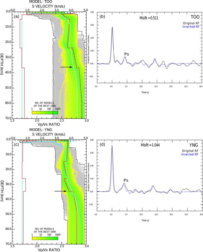
468                                                                    M. Bello et al.: Crustal structure of southeast Australia

                                                                      for the station. s(H, κ) achieves its maximum value when
                                                                      all three phases stack constructively, thereby producing es-
                                                                      timates for H and Vp /Vs beneath the station (see Figs. 5
                                                                      and S1–S4). In this study, the weighting factors used are
                                                                      w1 = 0.6, w2 = 0.3, and w3 = 0.1. The H –κ approach re-
                                                                      quires an estimate of the mean crustal P -wave velocity,
                                                                      which is used as an initial value. Based on the results of a
                                                                      previous seismic refraction study (Drummond and Collins,
                                                                      1986), we use an average crustal velocity of Vp = 6.65 km/s
                                                                      to obtain our estimates of H and κ in the study area, not-
                                                                      ing that H –κ stacking results are much more dependent on
                                                                      Vp /Vs than Vp (Zhu and Kanamori, 2000). To estimate the
                                                                      uncertainties in the H –κ stacking results, we compute the
                                                                      standard deviation of the H and κ values at each station.
                                                                      When only a small number of RFs are available at a station
                                                                      (e.g. four in the case of MILA), the estimates are unlikely to
                                                                      be particularly robust, and in such instances, they are perhaps
                                                                      best viewed as a lower bounds on uncertainty.
                                                                         While simple to implement, the Zhu and Kanamori (2000)
Figure 3. Distribution of distant earthquakes (teleseisms) used in    method can suffer from large uncertainties due to its as-
this study. The locations of events that are ultimately used for RF   sumption of a simple flat-laying layer over a half-space with
analysis are denoted by yellow dots. Concentric circles are plot-
                                                                      constant crustal and upper-mantle properties. Consequently,
ted at 30◦ intervals from the centre of Bass Strait. Topography and
                                                                      there are only two search parameters (H and κ) plus a priori
bathymetry colours are based on the ETOPO1 dataset (Amante and
Eakins, 2009).                                                        information (Vp , weightings), and this method does not ac-
                                                                      count for variation with back-azimuth. These problems can
                                                                      cause non-unique and inaccurate estimates, which can lead
5.2   H –κ stacking                                                   to potentially misleading interpretations; for instance, a low-
                                                                      velocity upper-crustal layer can appear as a very shallow
Having obtained reliable P -wave RFs, the H –κ stacking               Moho in an H –κ stacking search space diagram. Also, a dip-
technique is used to estimate crustal thickness and bulk              ping Moho and/or anisotropic layers within the crust can con-
Vp /Vs for individual stations. We apply the method of Zhu            tribute to uncertainty.
and Kanamori (2000) to stations where the direct P s (Moho
P to S conversion) phase and its multiples are observed. This
technique makes use of a grid search to determine the crustal         5.3   Non-linear waveform inversion
thickness (H ) and Vp /Vs (κ) values that correspond to the
peak amplitude of the stacked phases. A clear maximum re-             In an effort to refine the crustal model, we invert a stack of
quires a contribution from both the primary phase (P s) and           the radial RFs by adopting the workflow described by Shibu-
the associated multiples (PpP s). In the absence of multiples,        tani et al. (1996). We divide the waveform data (RFs) into
the maximum becomes smeared out due to the inherent trade-            four 90◦ quadrants based on the back-azimuth of their incom-
off between crustal thickness (H ) and average crustal veloc-         ing energy. The first quadrant back-azimuth range is from 0
ity properties (κ) (Ammon et al., 1990; Zhu and Kanamori,             to 90◦ , and an equivalent range in a clockwise direction de-
2000). The H –κ stacking algorithm reduces the aforemen-              fines the consecutive quadrants. The second and third quad-
tioned ambiguity by summing RF amplitudes for P s and its             rants (southeastern and southwestern back-azimuths) have
multiples – PpP s and PpSs + P sP s – at arrival times cor-           very small numbers of RFs. Data from the first and fourth
responding to a range of H and Vp /Vs values. In the H –κ             quadrants are of better quality, with the first quadrant show-
domain, the equation for stacking amplitude is                        ing more coherency than the fourth quadrant, which is likely
                                                                      due to the orientation of surrounding tectonic plate bound-
             N
             X                                                        aries; hence, the pattern of P -wave energy radiated towards
s (H, κ) =          w1 rj (t1 ) + w2 rj (t2 ) + w3 rj (t3 ) ,   (1)
             j =1
                                                                      Australia. Kennett and Furumura (2008) showed that seismic
                                                                      waves arriving in Australia from the northern azimuths un-
where rj (ti ); i = 1, 2, 3 are the RF amplitude values at            dergo multiple scattering but low intrinsic attenuation due to
the expected arrival times t1 , t2 , and t3 of the P s, PpP s,        heterogeneity in the lower crust and mantle; this tends to pro-
and PpSs + P sP s phases respectively for the j th RF; w1 ,           duce prolonged high-frequency coda. An important assump-
w2 , and w3 are weights based on the signal-to-noise ratio            tion in our inversion is that we neglect anisotropy and possi-
(w1 + w2 + w3 = 1); and N is the total number of radial RFs           ble Moho dip, which we assume have a second-order influ-

Solid Earth, 12, 463–481, 2021                                                            https://doi.org/10.5194/se-12-463-2021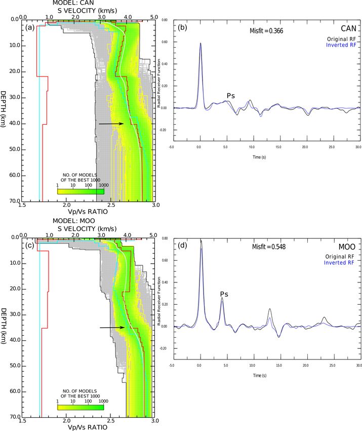
M. Bello et al.: Crustal structure of southeast Australia                                                                      469

                                                                    rameters required by NA: (1) the number of models produced
                                                                    per iteration (ns ); and (2) the number of neighbourhoods re-
                                                                    sampled per iteration (nr ). After a number of trials, we chose
                                                                    the maximum number of iterations to be 5500, with ns = 13
                                                                    and nr = 13 for all iterations. We employ a chi-square χ 2
                                                                    metric (see Sambridge, 1999a, for more details) to compute
                                                                    the misfit function, which is a measure of the inconsistency
                                                                                                               pre
                                                                    between the true (φiobs ) and predicted (φi (m)) waveforms
                                                                    for a given model m:
                                                                                                pre
                                                                                                     !
                                                                                   Nd
                                                                                1X    φiobs − φi (m)
                                                                    χν2 (m) =                          ,                       (2)
                                                                                ν i=1        σi

                                                                    where σi represents the noise standard deviation determined
                                                                    from φiobs , following the method described in Gouveia and
Figure 4. Stacked receiver functions from the Australian National   Scales (1998); and ν represents the number of degrees of
Seismic Network (ANSN) stations TOO, YNG, and MOO as well           freedom (the difference between the number of observations
as the Global Seismographic Network (GSN) station TAU. Small        and the number of parameters being inverted for). Using the
arrows indicate the arrival of the P s (black), PpP s (red), and
                                                                    above-mentioned parameters, the inversion targets the 1-D
PpP s + P sP s (blue) phases from the Moho.
                                                                    structure that produces the best fit between the predicted and
                                                                    observed RF. Figures 7–9 and S5–S9 present example results
                                                                    of inversions via density plots of the best 1000 data-fitting
ence on the waveforms that we use to constrain 1-D models           S-wave velocity models produced by the NA. The optimum
of the crust and upper mantle.                                      data-fitting model is plotted in red.
   Visual examination of coherency in P to S conversions al-
lows us to select a subset of RF waveforms for subsequent
stacking. This resulted in groups of mutually coherent wave-        6   Results
forms after which a move-out correction is then applied to
remove the kinematic effect of different earthquake distances       6.1 H –κ stacking results
prior to stacking using a cross-correlation matrix approach
described in Chen et al. (2010) and Tkalčić et al. (2011). Our    Maps of crustal thicknesses and average Vp /Vs from H –κ
visual acceptance criteria yields RFs at only 14 out of the         stacking in southeast Australia from 16 stations are shown
32 stations used for this study. An example of some stacked         in Fig. 6. At the remaining stations, we could not detect any
RFs is given in Fig. 4.                                             clear multiples or Moho conversions in the RFs from any di-
   We invert RFs for 1-D seismic velocity structure beneath         rection. A previous study by Chevrot and van der Hilst (2000)
selected seismic stations using the neighbourhood algorithm         has noted that this region is devoid of clear multiples. The
(NA) (Sambridge, 1999a, b) in order to better understand the        crustal thickness for all analysed stations in the study area
internal structure of the crust and the nature of the transition    varies from 23.2 ± 5.0 km (BA02) beneath northwestern Tas-
to the upper mantle. NA makes use of Voronoi cells to help          mania to 39.1 ± 0.5 km (CAN) beneath the Lachlan Fold
construct a searchable parameter space, with the aim of pref-       Belt, and the variation is strongly correlated with topogra-
erentially sampling regions of low data misfit. In the inver-       phy. Crust beneath VanDieland (Fig. 6a) is thin in the north
sion process, a Thomson–Haskell matrix method (Thomson,             (∼ 37.5 km) and south (∼ 33 km), but it appears to be consid-
1950; Haskell, 1953) was used to calculate a synthetic ra-          erably thinner beneath the Victorian and Tasmanian margin
dial RF for a given 1-D (layered) structure. During the inver-      Bass Strait (∼ 25 km). The mountainous region of the Lach-
sion, as in Shibutani et al. (1996) and Clitheroe et al. (2000),    lan Fold Belt has the deepest Moho at 39.1 ± 0.5 km (CAN)
each model is described by six layers: a layer of sediment; a       and a corresponding Vp /Vs value of 1.73 ± 0.02. Crust that is
basement layer; an upper crust, middle crust and lower crust;       consistently between ∼ 31 and 33 km thick lies beneath the
and an underlying mantle layer, all of which feature velocity       East Tasmania Terrane and eastern Bass Strait (ETT + EB).
gradients and, potentially, velocity jumps across boundaries.       The Vp /Vs ratio varies between ∼ 1.65 beneath station BA11,
The inversion involves constraining 24 parameters: Vs values        which also exhibits the thinnest crust, and ∼ 1.93 beneath
at the top and bottom of each layer, layer thickness, and the       stations BA19 and BA20 in southern Victoria. There is no
Vp /Vs ratio in each layer (Table 1). The inclusion of Vp /Vs       obvious correlation between the number of RFs used in the
ratio as an unknown primarily aims to accommodate the ef-           H –κ stacking and the size of the uncertainty in either the
fects of a sediment layer with limited prior constraints (Ban-      Moho depth or Vp /Vs , but as mentioned previously, the un-
nister et al., 2003). There are two important controlling pa-       certainty estimates for stations with a low number of RFs are

https://doi.org/10.5194/se-12-463-2021                                                           Solid Earth, 12, 463–481, 2021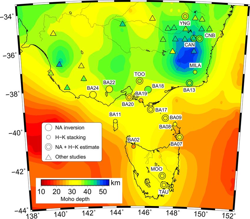
470                                                                          M. Bello et al.: Crustal structure of southeast Australia

Figure 5. Results from the H –κ stacking analysis for RFs (Zhu and Kanamori, 2000) at MOO, CAN, and TOO stations. (a) Normalized
amplitudes of the stack over all back-azimuths along the travel time curves corresponding to the P s and PpP s phases for each case. (b) The
corresponding stacked receiver function for each station.

                                                                                                       upper
Table 1. Model parameter bounds used in the neighbourhood algorithm receiver function inversion. Vs           and Vslower represent the S- wave
velocity at the top and bottom of a layer respectively. Vp /Vs represents the P - and S-wave velocity ratio within a layer.

                                                                   upper
                               Layer           Thickness (m)     Vs        (km/s)   Vslower (km/s)       Vp /Vs
                               Sediment                   0–2           0.5–1.5           0.5–1.5    2.00–3.00
                               Basement                   0–3           1.8–2.8           1.8–2.8    1.65–2.00
                               Upper crust               3–20           3.0–3.8           3.0–3.9    1.65–1.80
                               Middle crust              4–20           3.4–4.3           3.4–4.4    1.65–1.80
                               Lower crust               5–15           3.5–4.8           3.6–4.9    1.65–1.80
                               Mantle                    5–20           4.0–5.0           4.0–5.0    1.70–1.90

likely to be less robust. Table 2 shows a summary of the H –κ              refraction (Collins, 1991; Collins et al., 2003) studies. We
stacking results for the stations that have been analysed.                 also adopt an upper-mantle velocity of Vp = 7.6 km/s (i.e.
                                                                           Vs = 4.3–4.4 km/s for Vp /Vs ratios of 1.73–1.77 at the base
6.2   Non-linear inversion results                                         of the Moho gradient) following Clitheroe et al. (2000), who
                                                                           used this value for RF studies, and Collins et al. (2003), who
Results of the NA inversion were successfully obtained for                 used Vp > 7.8 km/s for their summary of both seismic re-
a selection of permanent and temporary stations, as shown                  fraction and RF results; these Vp values are consistent with
in Table 2 and Fig. 10. If the Moho is defined by a gentle                 global Earth models (e.g. Kennett et al., 1995). Therefore, we
velocity gradient, the base of the velocity gradient is used               also require the S-wave velocity to be > ∼ 4.4 km/s beneath
as a proxy for the Moho depth, as done in previous RF (e.g.                the Moho. We present the S-wave velocity profiles from the
Clitheroe et al., 2000; Fontaine et al., 2013a) and seismic

Solid Earth, 12, 463–481, 2021                                                                  https://doi.org/10.5194/se-12-463-2021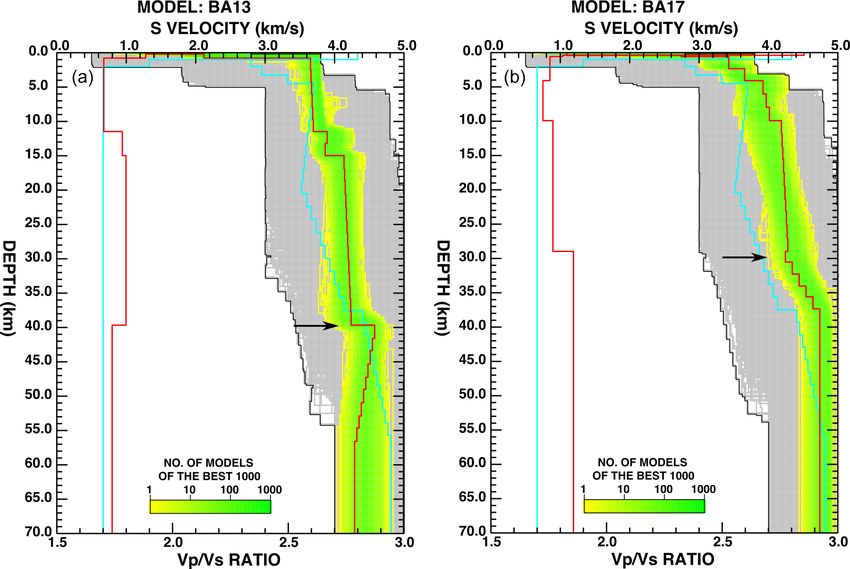
M. Bello et al.: Crustal structure of southeast Australia 471
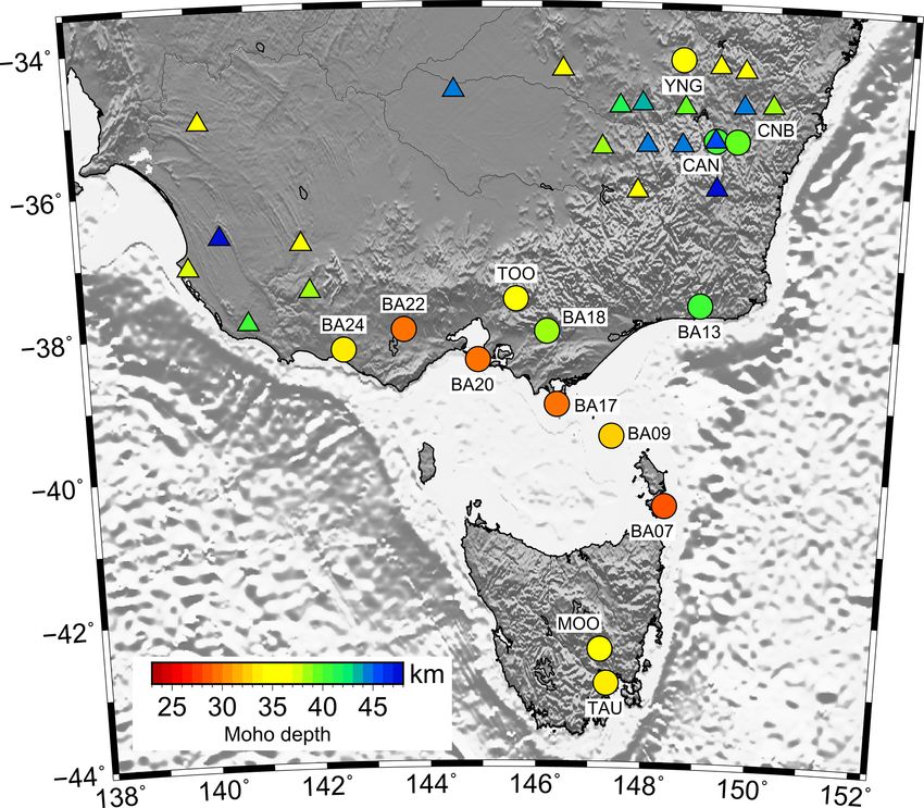
Figure 6. (a) Variations in the crustal thickness and (b) Vp /Vs ratio taken from the linear (H –κ) stacking results (Table 2). Crustal thickness
varies between ∼ 23 and 39 km. The Vp /Vs ratios vary from ∼ 1.65 to 1.93. The thick black dashed line denotes the boundary of VanDieland.
The thick magenta dashed line outlines the boundary of the East Tasmania Terrane and eastern Bass Strait (ETT + EB). The thick cyan
dashed line highlights the eastern part of the Lachlan Fold Belt. The illuminated topography and bathymetry are based on the ETOPO1
dataset (Amante and Eakins, 2009).
Table 2. Summary of H –κ stacking and NA inversion results for the current study.
Basic station information Results
Type Station name Lat (◦ ) Long (◦ ) No. of Moho depth (km) Bulk Vp /Vs Moho depth (km) Quality Moho type
RFs (H –κ stacking) (H –κ stacking) (NA inversion) (NA inversion) (NA inversion)
BA02 −40.95 145.20 9 23.2 ± 5.0 1.83 ± 0.31 – Moderate Not evident
BA03 −41.20 145.84 8 – – – Moderate Not evident
BA07 −40.43 148.31 6 32.5 ± 0.1 1.70 ± 0.02 28 Good Sharp
BA08 −39.77 147.97 8 31.9 ± 0.1 1.70 ± 0.07 – Poor –
Temporary stations
BA09 −39.47 147.32 8 32.8 ± 1.7 1.71 ± 0.07 32 Good Sharp
BA11 −39.64 143.98 12 30.5 ± 2.1 1.65 ± 0.07 – – –
BA13 −37.63 148.83 24 37.7 ± 2.9 1.74 ± 0.10 40 Good Sharp
BA17 −39.04 146.33 20 30.9 ± 2.5 1.76 ± 0.10 29 Good Broad
BA18 −38.02 146.14 3 – – 38 Good Sharp
BA19 −38.57 145.69 20 25.5 ± 2.4 1.93 ± 0.14 – Good Not evident
BA20 −38.42 144.92 30 26.3 ± 1.6 1.93 ± 0.12 29 Good Sharp
BA22 −37.99 143.61 5 – – 29 Poor Sharp
BA24 −38.26 142.54 4 – – 33 Poor Sharp
TAU −42.91 147.32 41 33.5 ± 1.9 1.70 ± 0.08 33 Poor Intermediate
Permanent stations
MOO −42.44 147.19 58 33.0 ± 1.2 1.71 ± 0.04 34 Good Sharp
TOO −37.57 145.59 276 37.5 ± 1.2 1.68 ± 0.04 36 Good Sharp
YNG −34.20 148.40 178 37.3 ± 0.5 1.76 ± 0.04 35 Good Sharp
CAN −35.32 149.00 402 39.1 ± 0.5 1.73 ± 0.02 40 Good Sharp
CNB −35.32 149.36 155 38.5 ± 1.1 1.70 ± 0.04 39 Good Broad
MILA −37.05 149.16 4 37.6 ± 2.1 1.73 ± 0.06 – – –
NA inversion for stations CAN, MOO, TOO, YNG, BA13, between the synthetic and observed RF. Models that fail to fit
and BA17 in Figs. 7–9 as well as the observed and predicted significant arrivals in the observed RF are rejected. Based on
RFs. The S-wave velocity inversion results for the remain- these criteria, the inversion results are classified as follows:
ing stations are included in the Supplement (Figs. S5–S8). In
assigning the Moho depth, we consider three criteria to ex-
amine the quality of the inversion result: (1) misfit value χ 2 ;
(2) the quality of the RF stack (which is based on our ability
to pick the direct and multiple phases); and (3) the visual fit
https://doi.org/10.5194/se-12-463-2021 Solid Earth, 12, 463–481, 2021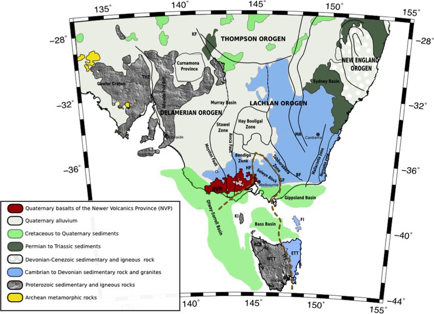
472                                                                  M. Bello et al.: Crustal structure of southeast Australia

    – very good – very low χ 2 (typically < 0.4), very good         the nature of the Moho, and crustal velocity and velocity ra-
      visual fit to direct and multiple phases;                     tio variations from H –κ stacking and the 1-D S-wave ve-
                                                                    locity models. Overall, the agreement between Moho depths
    – good – low χ 2 (typically 0.4–0.8), direct phases clearly     obtained from the H –κ stacking results and NA inversion
      visible, multiple phases less clear, and a good visual fit    is generally within error (Table 2), which makes a joint in-
      to all major identifiable phases;                             terpretation more straightforward. Comparison is also made
                                                                    to other studies that have examined crustal seismic proper-
    – poor – medium to high χ 2 (in the range 0.8–1.2), direct
                                                                    ties in southeast Australia, and we attempt to integrate our
      phases visible, multiple phases unclear, and moderate
                                                                    new findings with previous results from teleseismic tomog-
      visual fit to some identifiable phases.
                                                                    raphy, SKS splitting, and ambient noise tomography in order
   In general, the optimum χ 2 value is normally considered         to better understand the crust and upper-mantle structure and
to be 1, as below this value, the tendency is to fit noise rather   dynamics beneath this region.
than signal. However, this is for the ideal case when the num-
ber of degrees of freedom and the absolute values of the            7.1   Lateral variation in crustal thickness and the
data uncertainty are well known (e.g. in the case of a syn-               nature of the Moho
thetic test). In the case of observational data, these values
are often poorly constrained, so using the relative χ 2 val-        The RF analysis clearly reveals the presence of lateral
ues coupled with visual assessment of the data fit appears          changes in crustal thickness that span mainland Australia
to be reasonable. With regard to the character of the crust–        through Bass Strait to Tasmania (Figs. 6 and 10; in the lat-
mantle transition, this study classifies the transition zone as     ter case, RF depths from previous studies are also included
sharp ≤ 2 km, intermediate 2–10 km, or broad ≥ 10 km, as            for reference). The stations located in the Palaeozoic Lachlan
initially proposed by Shibutani et al. (1996) and modified by       Fold Belt reveal a generally thick crust that ranges between
Clitheroe et al. (2000).                                            ∼ 37 and 40 km. Although the Moho was picked as a ve-
   We note that for the seven permanent stations for which          locity jump for stations YNG, CAN, and CNB, the velocity
we produce receiver function inversion and H –κ stacking            nonetheless tends to continue to increase with depth below
results, five have estimates of the Moho depth from previ-          the discontinuity. This, coupled with the fact that Clitheroe
ous receiver function studies. Clitheroe et al. (2000) esti-        et al. (2000) estimate the Moho to be almost 10 km deeper
mated the Moho depth at 49 km beneath CAN based on a                beneath CAN, is consistent with the presence of mafic un-
non-linear inversion, which is ∼ 10 km greater than the re-         derplating (e.g. Drummond and Collins, 1986; Shibutani et
sults we obtain for both NA inversion and H –κ stacking             al., 1996; Clitheroe et al., 2000), sourced from the ambient
(see Sect. 7.1 for further discussion of this discrepancy).         convecting mantle. The top and bottom of such a layer could
Ford et al. (2010) determined the Moho depth beneath the            feature a velocity step with depth, and its internal structure
MOO, TOO, TAU, and YNG stations using H –κ stacking                 is likely to be layered and/or gradational, resulting in un-
and found values (compared with our H –κ stacking results)          certainty in the true Moho depth. Based on deep crustal re-
of 33 ± 3 km (33.0 ± 1.2 km), 34 ± 3 km (37.5 ± 1.2 km),            flection profiling, Glen et al. (2002) suggested that the deep
32 ± 3 km (33.5 ± 1.9 km), and 33 ± 2 km (37.3 ± 0.5 km)            Moho underlying the Lachlan Orogen results from magmatic
respectively. These are all within error, with the slight ex-       underplating that added a thick Ordovician mafic layer at the
ception of YNG station, located in Young, on the western            base of the crust coupled with a thick sequence of Ordovician
flanks of the Great Dividing Range, where we might expect           mafic rocks that can be found in the mid and lower crust. Fin-
the crust to be slightly thicker than average. Overall, how-        layson et al. (2002) and Glen et al. (2002) also inferred the
ever, these similarities suggest that our results are likely to     presence of underplating near CNB and CAN from seismic
be robust.                                                          refraction data. Collins (2002) postulated that the underplat-
                                                                    ing might have occurred in the back-arc region of a subduc-
                                                                    tion zone due to pronounced adiabatic decompression melt-
7     Discussion                                                    ing in the asthenosphere. The seismic tomography model of
                                                                    Rawlinson et al. (2010, 2011) exhibits an increase in P -wave
For convenience, the seismic stations are separated into three      speed at 50 km depth beneath CAN, CNB, and YNG, and the
groups (Fig. 2) based on tectonic setting and the results ob-       authors suggest that magmatic underplating may be the cause
tained. Stations YNG, CAN, CNB, MILA, and BA13 are lo-              of the high-velocity anomaly. A recent study by Davies et
cated in the Lachlan Fold Belt; stations BA02, BA11, BA19,          al. (2015) identified the longest continental hotspot track in
BA20, TAU, MOO, and TOO sit above the VanDieland mi-                the world (over 2000 km total length), which began in north
crocontinental block; and stations BA07, BA08, BA09, and            Queensland at ∼ 33 Ma, and propagated southward under-
BA17 lie in the East Tasmania Terrane and eastern Bass              neath the present-day Lachlan Fold Belt and Bass Strait. The
Strait (ETT + EB). Stations BA22 and BA24 lie to the west           magmatic underplating could therefore be a consequence of
of VanDieland. This discussion focuses on crustal thickness,        the passage of the continent above a mantle upwelling lead-

Solid Earth, 12, 463–481, 2021                                                          https://doi.org/10.5194/se-12-463-2021
M. Bello et al.: Crustal structure of southeast Australia 473 Figure 7. (a, c) Seismic velocity models for the CAN and MOO stations obtained from the neighbourhood algorithm (Sambridge, 1999a). The grey area indicates all the models searched by the algorithm. The best 1000 models are indicated by the yellow to green colours; the best model (smallest misfit) is shown using the red line, for both the S-wave velocity (top x axis) and Vp /Vs ratio (bottom x axis), and the white line is the average velocity model. Small black arrows denote the estimated depth of the Moho. (b, d) Waveform matches between the observed stacked receiver functions (black) and predictions (blue) based on the best models. “Misfit” refers to the chi-square estimate as defined by Eq. (2). ing to a more diffuse crust–mantle transition zone. The thick- before increasing to ∼ 33 km in southern Tasmania. The ened crust and a transitional Moho observed in the Lach- results in southern Tasmania agree with those of Korsch lan Fold Belt are consistent with the proposed delamination et al. (2002) from a seismic reflection profile adjacent to models of Collins and Vernon (1994). the TAU and MOO seismic stations. The thinner crust be- Strong lateral changes in crustal seismic structure (Figs. 6, neath Bass Strait and its margins may be a consequence 10) beneath VanDieland appear to be a reflection of the re- of lithospheric thinning and/or delamination associated with gion’s complex tectonic history. The thick crust (∼ 37 km) failed rifting that accompanied the break-up of Australia and beneath the Selwyn Block (see Fig. 1 for its location) – Antarctica (Gaina et al., 1998). Stations BA07, BA08, BA09, within the northern margin of VanDieland in southern Vic- and BA17 (ETT + EB) collectively indicate crust of rela- toria – thins dramatically to ∼ 26 km as it enters Bass tive uniform thickness (∼ 31–32 km; Fig. 10a, b). Relative Strait, increases to ∼ 30 km beneath King Island (BA11), to western Bass Strait, the crust is slightly thicker in this part and then thins to ∼ 23 km beneath northwestern Tasmania, of the study area, which may suggest underplating associ- https://doi.org/10.5194/se-12-463-2021 Solid Earth, 12, 463–481, 2021
474                                                                    M. Bello et al.: Crustal structure of southeast Australia

Figure 8. (a, c) Seismic velocity models for TOO and YNG stations obtained from the neighbourhood algorithm. (b, d) Comparison between
the observed stacked and the predicted receiver functions from the NA inversion. See the caption of Fig. 7 for more details.

ated with a Palaeozoic subduction system (e.g. Drummond              creasing SiO2 content in the continental crust (Christensen,
and Collins, 1986; Gray and Foster, 2004).                           1996), and (2) partial melt is revealed by elevated Vp /Vs , es-
   In general, our understanding of crustal thickness varia-         pecially if the anomaly is localized to an intra-crustal layer
tions are limited by station separation, so it is difficult to de-   (Owens and Zandt, 1997). A more felsic (SiO2 ) composition
termine whether smooth variations in thickness or step-like          in the lower crust is represented by a lower Vp /Vs , which
transitions explain the observations.                                reflects removal of an intermediate-mafic zone by delamina-
                                                                     tion, whereas a more mafic lower crust is revealed by higher
7.2   Vp /Vs and bulk crustal composition                            Vp /Vs (> 1.75) which may be due to underplated material
                                                                     (Pan and Niu, 2011). However, lower crustal delamination
Vp /Vs can constrain chemical composition and mineralogy             can also result in decompression melting, which can yield
more robustly than P - or S-wave velocity in isolation (Chris-       elevated Vp /Vs (He et al., 2015). We interpret the variation
tensen and Fountain, 1975). We observe variations in Vp /Vs          of observed Vp /Vs in the southern Tasmanides to be a conse-
across the study region, which we can largely equate with            quence of compositionally heterogeneous crust and localized
variations in composition or melt. Studies in mineral physics        partial melt that may likely be sourced from recent intraplate
and field observations show (1) an increase in Vp /Vs with de-       volcanism (Rawlinson et al., 2017).

Solid Earth, 12, 463–481, 2021                                                            https://doi.org/10.5194/se-12-463-2021
M. Bello et al.: Crustal structure of southeast Australia 475
Figure 9. Seismic velocity models for temporary stations BA13 (a) and BA17 (b) obtained from the neighbourhood algorithm. See Figs. S6–
S9 in the Supplement for all receiver function inversion results for the temporary BASS network, including waveform fits (Supplement
Fig. S7 includes the waveform fit for stations BA13 and BA17).
Figure 6b shows the distribution of bulk Vp /Vs across the
study area. The pattern of Vp /Vs ratios appears to delin-
eate three distinct zones of crust. Beneath the Lachlan Oro-
gen, values are ∼ 1.75, which is consistent with the pres-
ence of a mafic lower crust, as suggested by a number of
other studies (Drummond and Collins, 1986; Shibutani et al.,
1996; Clitheroe et al., 2000; Finlayson et al., 2002). Beneath
eastern Bass Strait, the Vp /Vs ratios are slightly lower, with
BA07, BA08, and BA09 exhibiting values of 1.70, 1.70, and
1.71 respectively. These values are in agreement with con-
straints from seismic reflection and refraction studies (Fin-
layson et al., 2002; Collins et al., 2003) and may indicate
a felsic to intermediate crustal composition. The geology
of Flinders Island, which hosts both BA07 and BA08, is
dominated by Devonian granites, which is consistent with
this observation. Beneath VanDieland, Vp /Vs is highly vari-
able, with the greatest contrast between BA11 (∼ 1.65) and
BA19/20 (∼ 1.93), and BA19/20 and TOO (1.68). BA11 is
located on King Island, which is characterized by Precam-
brian and Devonian granite outcrops, which may help explain
the low Vp /Vs . The high Vp /Vs beneath BA19/20 is harder to
explain but could be caused by melt in the crust associated
Figure 10. Map showing crustal thickness variations based on the
with the Newer Volcanics Province, which sits along the Cos-
S-wave velocity inversion results of this study (circles) and pre-
grove intraplate volcanic track and last erupted only ∼ 4.6 ka
vious studies (triangles) (Clitheroe et al., 2000; Fontaine et al.,
2013a, b; Shibutani, 1996; Tkalcic et al., 2012). The topography and (Rawlinson et al., 2017). The return to lower Vp /Vs beneath
bathymetry are based on the ETOPO1 dataset (Amante and Eakins, TOO over a relatively short distance (∼ 100 km) is also dif-
2009). ficult to explain, but we note that this region of Victoria is
underlain by granite intrusions.
https://doi.org/10.5194/se-12-463-2021 Solid Earth, 12, 463–481, 2021476 M. Bello et al.: Crustal structure of southeast Australia
In summary, the crust beneath VanDieland exhibits the
greatest lateral heterogeneity in Vp /Vs , which likely reflects
considerable variations in composition and the presence of
melt. This can partially be explained by the tectonic history
of the region, which includes failed rifting in Bass Strait ac-
companied by widespread magma intrusion and granite em-
placement as well as, more recently, the passage of a plume
(Rawlinson et al., 2017). Furthermore, Moore et al. (2015)
used reflection transects and potential field data to infer that
VanDieland is comprised of up to seven continental ribbon
terranes that are bounded by major faults and suture zones,
which were likely amalgamated by the end of the Protero-
zoic. Hence, considerable variations in composition and, in
turn, Vp /Vs ratio are to be expected.
7.3 Moho depth comparison
Prior to this study, a variety of seismic methods have been
used to constrain the Moho depth in southeast Australia,
Figure 11. Comparison between the AusMoho model (background
including receiver functions, reflection profiling, and wide-
colour map) and the Moho depths determined through RF analysis
angle refection and refraction experiments. In an effort to in this and previous studies. Small coloured circles denote the Moho
combine the results from all of these studies into a single syn- depths determined from H –κ stacking, whereas large coloured cir-
thesis, Kennett et al. (2011) developed the AusMoho model; cles correspond to receiver function estimates. When both H –κ-
this included Moho depth estimates from over 11 000 km of and NA-derived depths are available at a single station, the smaller
reflection transects across the continent, numerous refraction H –κ circle is superimposed on the larger NA circle so that both
studies, and 150 portable and temporary stations. Due to ir- depths can be observed on the one plot. Moho depths determined
regular sampling, the detail of this model is highly variable; from previous RF studies are denoted by triangles.
for example, the region beneath Bass Strait is constrained by
only five measurements, whereas the central Lachlan Fold
Belt around Canberra (see Fig. 1 for location) features rela-
tively dense sampling at ∼ 50 km intervals or less. which can effectively yield two options for the Moho transi-
AusMoho includes previous receiver function results from tion due to an expected high Vp /Vs (> 1.85) in the underplate
Shibutani et al. (1996), Clitheroe et al. (2000), Fontaine et layer (e.g. Cornwell et al., 2010). AusMoho Moho depths be-
al. (2013a), and Tkalcic et al. (2012), as well as reflection and neath BA07 and BA08 are considerably shallower than our
refraction transects in Tasmania, parts of the Lachlan Oro- estimates, which we attribute to a lack of data coverage in
gen, and western Victoria. Figure 11 illustrates AusMoho for this region. Sizable discrepancies also exist beneath BA02,
our study region, which exhibits large variations in the Moho BA19, and BA20: in the former case, the uncertainty in our
depth (from ∼ 10 to > 50 km). These extremes are due to H –κ stacking estimate is 5 km, which may be a factor here;
the presence of oceanic crust outboard of the passive margin in the latter case, we also note that there is sparse data cov-
of the Australian continent, and the root beneath the South- erage southeast of Melbourne to constrain AusMoho, so it
ern Highlands, which represent the southern extension of the would appear that our new Moho depths are more likely to
Great Dividing Range in New South Wales. Superimposed be correct. Overall, while there is good consistency between
on Fig. 11 are Moho depths from the four previous receiver AusMoho and our new results, any updated version of Aus-
function studies cited above as well as NA inversion and H – Moho should incorporate the Moho depth estimates from this
κ depth estimates from this study. As expected, the correla- study.
tion between the previous RF results and AusMoho is gen- Although AusMoho did make use of results from a 3-D
erally good, as they were part of the dataset used to build wide-angle reflection and refraction survey of Tasmania (off-
this model. In places where they do not match, this can be shore shots and onshore stations), it only used a few sample
attributed to the presence of seismic refraction or reflection points for the final Moho model (Kennett et al., 2011); there-
lines that were also used to constrain AusMoho. fore, the resolution of AusMoho is considerably less than the
In general, the agreement between the results from this Moho model produced by Rawlinson et al. (2001). Conse-
study and AusMoho is good, but there are exceptions. For quently, we plot our three RF results on top of this model
instance, CAN, CNB, YNG, and MILA tend to be somewhat in the Supplement (Fig. S10). The agreement between the
shallower than AusMoho. However, this can be attributed to Moho model and RF depths beneath MOO and TAU is good,
the likely presence of mafic underplating alluded to earlier, but RF estimates beneath BA02 are shallower than the Moho
Solid Earth, 12, 463–481, 2021 https://doi.org/10.5194/se-12-463-2021You can also read