Toward Increased Airspace Safety: Quadrotor Guidance for Targeting Aerial Objects - arXiv
←
→
Page content transcription
If your browser does not render page correctly, please read the page content below
Toward Increased Airspace Safety: Quadrotor
arXiv:2107.01733v1 [cs.RO] 4 Jul 2021

                                           Guidance for Targeting Aerial Objects
                                                           Anish Bhattacharya
                                                            CMU-RI-TR-20-39
                                                                August 2020

                                                         School of Computer Science
                                                         Carnegie Mellon University
                                                            Pittsburgh, PA 15213

                                                            Thesis Committee:
                                                          Sebastian Scherer (Chair)
                                                              Oliver Kroemer
                                                            Azarakhsh Keipour

                                              Submitted in partial fulfillment of the requirements
                                                     for the degree of Master of Science.

                                                     Copyright © 2020 Anish Bhattacharya
To my parents and my girlfriend for their constant support.
iv
Abstract
     As the market for commercially available unmanned aerial vehicles (UAVs) booms,
there is an increasing number of small, teleoperated or autonomous aircraft found in
protected or sensitive airspace. Existing solutions for removal of these aircraft are ei-
ther military-grade and too disruptive for domestic use, or compose of cumbersomely
teleoperated counter-UAV vehicles that have proven ineffective in high-profile domes-
tic cases. In this work, we examine the use of a quadrotor for autonomously targeting
semi-stationary and moving aerial objects with little or no prior knowledge of the tar-
get’s flight characteristics. Guidance and control commands are generated with infor-
mation just from an onboard monocular camera. We draw inspiration from literature
in missile guidance, and demonstrate an optimal guidance method implemented on a
quadrotor but not usable by missiles. Results are presented for first-pass hit success
and pursuit duration with various methods. Finally, we cover the CMU Team Tartan
entry in the MBZIRC 2020 Challenge 1 competition, demonstrating the effectiveness
of simple line-of-sight guidance methods in a structured competition setting.
vi
Acknowledgments
    I would like to thank my advisor, Prof. Sebastian Scherer, for his support and
guidance throughout the work involved in this thesis. I would also like to thank my
committee members, Prof. Oliver Kroemer and Azarakhsh Keipour for their consider-
ation and feedback. The advice, mentorship, and friendship provided by the members
of the AirLab and greater RI was a key element to my experience at CMU; specifically,
I would like to recognize Rogerio Bonatti, Azarakhsh Keipour, and Vai Viswanathan
for their help and guidance. John Keller was extremely helpful for setting up DJI SDK
integration as well as advising with random software challenges. Finally, I would like
to thank the members of CMU Team Tartans: Akshit Gandhi, Noah LaFerriere, Lukas
Merkle, Andrew Saba, Rohan Tiwari, Stanley Winata, and Karun Warrior. Jay Maier,
Lorenz Stangier, and Kevin Zhang also contributed to this effort.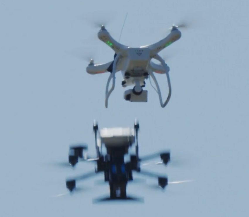
viii
Contents

1   Introduction                                                                                                       1
    1.1 Motivation . . . . . . . . . . . . . . . . . . . . . . . . . . . . . . . . . . . . . . .                       1
    1.2 Challenges and Approach . . . . . . . . . . . . . . . . . . . . . . . . . . . . . . .                          2
    1.3 Contribution and Outline . . . . . . . . . . . . . . . . . . . . . . . . . . . . . . .                         3

2   Related Work                                                                                                       5
    2.1 Classical Visual Servoing . . . . . . . . . . . . . . . . . . . . . . . . . . . . . . .                        5
    2.2 Missile Guidance . . . . . . . . . . . . . . . . . . . . . . . . . . . . . . . . . . .                         5
    2.3 Trajectory Generation and Tracking . . . . . . . . . . . . . . . . . . . . . . . . .                           7

3   Targeting Moving Objects with a Quadrotor                                                                          9
    3.1 Line-of-Sight Guidance . . . . . . . . . . . . . . . . . . . . . . .      .   .   .   .   .   .   .   .   .    9
         3.1.1 Derivation of True Proportional Navigation Guidance Law            .   .   .   .   .   .   .   .   .    9
         3.1.2 True Proportional Navigation . . . . . . . . . . . . . . .         .   .   .   .   .   .   .   .   .   11
         3.1.3 Proportional Navigation with Heading Control . . . . . .           .   .   .   .   .   .   .   .   .   12
         3.1.4 Hybrid TPN-Heading Control . . . . . . . . . . . . . . .           .   .   .   .   .   .   .   .   .   13
    3.2 Trajectory Following . . . . . . . . . . . . . . . . . . . . . . . .      .   .   .   .   .   .   .   .   .   14
         3.2.1 LOS 0 Acceleration Trajectory Following . . . . . . . . .          .   .   .   .   .   .   .   .   .   14
         3.2.2 Target Motion Forecasting . . . . . . . . . . . . . . . . .        .   .   .   .   .   .   .   .   .   15
    3.3 System . . . . . . . . . . . . . . . . . . . . . . . . . . . . . . . .    .   .   .   .   .   .   .   .   .   15
         3.3.1 Perception . . . . . . . . . . . . . . . . . . . . . . . . .       .   .   .   .   .   .   .   .   .   16
         3.3.2 Control . . . . . . . . . . . . . . . . . . . . . . . . . . .      .   .   .   .   .   .   .   .   .   19
         3.3.3 Simulation Package . . . . . . . . . . . . . . . . . . . . .       .   .   .   .   .   .   .   .   .   19
    3.4 Results . . . . . . . . . . . . . . . . . . . . . . . . . . . . . . . .   .   .   .   .   .   .   .   .   .   21
         3.4.1 First-Pass Hit Rates . . . . . . . . . . . . . . . . . . . . .     .   .   .   .   .   .   .   .   .   22
         3.4.2 Pursuit Duration . . . . . . . . . . . . . . . . . . . . . .       .   .   .   .   .   .   .   .   .   27
         3.4.3 Pursuit Behavior . . . . . . . . . . . . . . . . . . . . . .       .   .   .   .   .   .   .   .   .   29

4   LOS Guidance Applied in a Robotics Competition Setting                                                            33
    4.1 Introduction . . . . . . . . . . . . . . . . . . . . . . . . . . . . . . . . . . . . . .                      33
    4.2 Software System . . . . . . . . . . . . . . . . . . . . . . . . . . . . . . . . . . .                         34
        4.2.1 Perception . . . . . . . . . . . . . . . . . . . . . . . . . . . . . . . . . .                          34

                                                 ix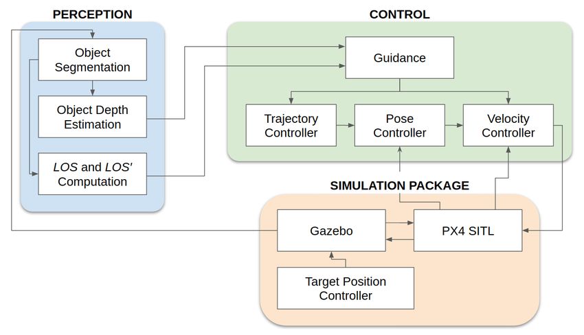
4.2.2 Planning, Guidance, and Control         .   .   .   .   .   .   .   .   .   .   .   .   .   .   .   .   .   .   .   .   .   .   .   35
          4.2.3 Drone Interface . . . . . . . . .       .   .   .   .   .   .   .   .   .   .   .   .   .   .   .   .   .   .   .   .   .   .   .   37
    4.3   Results . . . . . . . . . . . . . . . . . .   .   .   .   .   .   .   .   .   .   .   .   .   .   .   .   .   .   .   .   .   .   .   .   37
          4.3.1 Task 1 . . . . . . . . . . . . . .      .   .   .   .   .   .   .   .   .   .   .   .   .   .   .   .   .   .   .   .   .   .   .   37
          4.3.2 Task 2 . . . . . . . . . . . . . .      .   .   .   .   .   .   .   .   .   .   .   .   .   .   .   .   .   .   .   .   .   .   .   39

5   Conclusion                                                                                   41
    5.1 Discussion . . . . . . . . . . . . . . . . . . . . . . . . . . . . . . . . . . . . . . . 41
    5.2 Future Work . . . . . . . . . . . . . . . . . . . . . . . . . . . . . . . . . . . . . . 42

                                                  x
List of Figures
1.1 Current possible domestic-use counter-UAV systems in development. . . . . . . . 2
2.1 Constant-bearing collision course diagram with instantaneous lateral acceleration
applied to missile [1]. . . . . . . . . . . . . . . . . . . . . . . . . . . . . . . . . . 6
2.2 Comparison of pure and true proportional navigation. AM and VM refer to the
missile’s desired acceleration and current velocity, respectively [2]. . . . . . . . . . 6
2.3 Example of concatenated trajectories in a cluttered environment. Colored lines
represent individual motion primitives; the quadrotor tracks the initial part of every
generated trajectory, forming a complete, stitched trajectory represented by the
black line. [3] . . . . . . . . . . . . . . . . . . . . . . . . . . . . . . . . . . . . . 7
3.1 LOS coordinate system [4]. . . . . . . . . . . . . . . . . . . . . . . . . . . . . . . 10
3.2 Example image frame with detected object’s centroid at times t − 1 and t. . . . . . 11
3.3 Top-down diagram showing intermediate quantities in calculation of desired accel-
eration command. . . . . . . . . . . . . . . . . . . . . . . . . . . . . . . . . . . . 11
3.4 Diagram of trajectory replanning by stitching trajectory to the look ahead point.
UAV closely follows the tracking point. . . . . . . . . . . . . . . . . . . . . . . . 14
3.5 System diagram. . . . . . . . . . . . . . . . . . . . . . . . . . . . . . . . . . . . 16
3.6 Input and output of Object Segmentation node. . . . . . . . . . . . . . . . . . . . 16
3.7 Example image frame with detected object’s centroid and part of depth estimation
calculations. (ulef t , vlef t ) and (uright , vright ) points along image horizontal corre-
sponding to target edges are shown before (red) and after (black) rotation back into
the original segmented coordinates. Note that because of the wide field of view,
images around the edges of the image frame can get warped even though there is
no distortion in this camera model. . . . . . . . . . . . . . . . . . . . . . . . . . . 17
3.8 Top-down diagram showing calculation of estimated distance to object center d0
with 3D projected rays to target edges. . . . . . . . . . . . . . . . . . . . . . . . . 17
3.9 Gazebo simulation world, with UAV model and target in view. . . . . . . . . . . . 20
3.10 Target path library taken from similar perspectives. Dark blue sphere is the target’s
current position. Light blue sequence is the traced path. (a) straight path with
random slope; (b) figure-8 path with random tilt, of size 10m×6m; (c) knot path
with random center point, of size 2m×2m×2m. . . . . . . . . . . . . . . . . . . . 20
3.11 True Proportional Navigation hit rate across three target paths. . . . . . . . . . . . 22
xi3.12 Proportional Navigation with Heading Control hit rate across three target paths. . . 22
3.13 Hybrid True Proportional Navigation-Heading Control hit rate across three target
paths. . . . . . . . . . . . . . . . . . . . . . . . . . . . . . . . . . . . . . . . . . 23
3.14 LOS’ Trajectory hit rate across three target paths. . . . . . . . . . . . . . . . . . . 23
3.15 Forecasting Trajectory hit rate across three target paths. . . . . . . . . . . . . . . . 24
3.16 Demonstration of TPN, straight target path, UAV speed 2m/s and target speed 25%
(0.5m/s); corresponding datapoint is represented in top left corner of Figure 3.11a. . 26
3.17 Mean pursuit durations for straight target path. . . . . . . . . . . . . . . . . . . . . 27
3.18 Mean pursuit durations for figure-8 target path. . . . . . . . . . . . . . . . . . . . 28
3.19 Mean pursuit durations for knot target path. . . . . . . . . . . . . . . . . . . . . . 28
3.20 TPN behavior. . . . . . . . . . . . . . . . . . . . . . . . . . . . . . . . . . . . . . 29
3.21 PN-Heading behavior. . . . . . . . . . . . . . . . . . . . . . . . . . . . . . . . . . 30
3.22 Hybrid TPN-Heading behavior. . . . . . . . . . . . . . . . . . . . . . . . . . . . . 30
3.23 LOS’ Trajectory behavior. . . . . . . . . . . . . . . . . . . . . . . . . . . . . . . 31
3.24 Forecasting Trajectory behavior. . . . . . . . . . . . . . . . . . . . . . . . . . . . 31
4.1 Diagram of software system used on both Challenge 1 UAVs. . . . . . . . . . . . . 34
4.2 Global planner trajectory generated to search for balloons over the entire arena for
Task 1. Black lines indicate a forward pass starting from the START position, and
red lines indicate the shifted reverse pass. . . . . . . . . . . . . . . . . . . . . . . 36
4.3 Global planner trajectory generated to search for the ball in the center of the arena
for Task 2. Black lines indicate the pursuer UAV trajectory, with the black arrows
indicating yaw orientation (and therefore camera orientation). The yellow line is
the target UAV and ball path. . . . . . . . . . . . . . . . . . . . . . . . . . . . . . 36
4.4 Snapshots of Task 1 subtasks. . . . . . . . . . . . . . . . . . . . . . . . . . . . . . 39
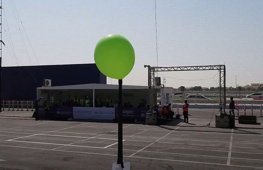
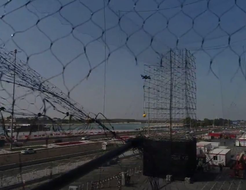
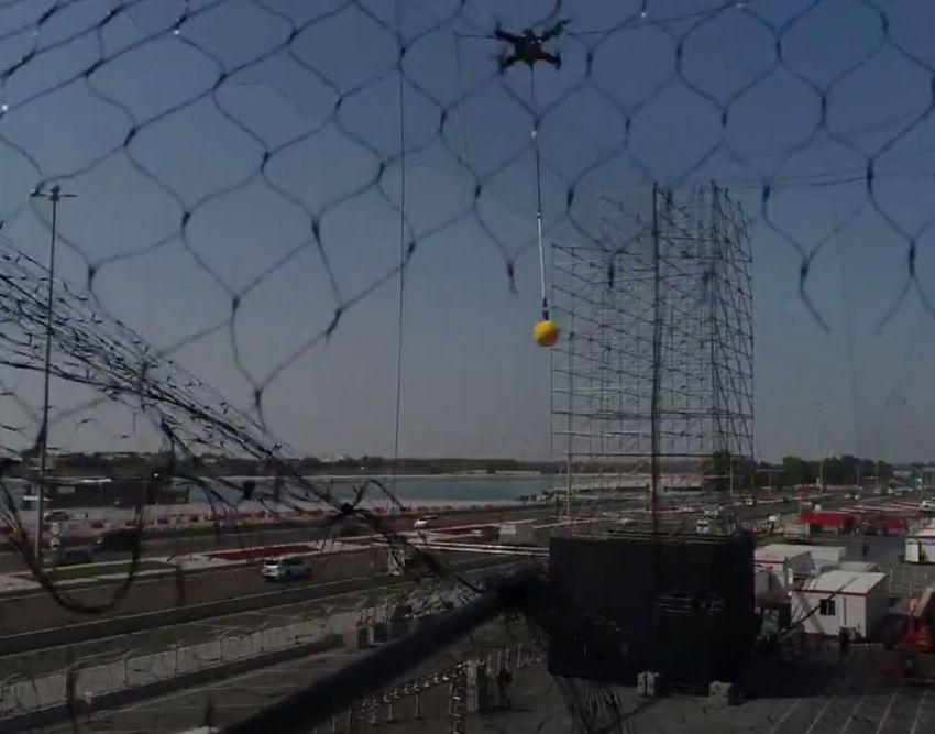
4.5 Target ball moving away from UAV in Task 2. Netting is part of a UAV-mounted
ball catcher. (a) LOS guidance issues a velocity command upwards, towards the
target to intercept it on the next pass; (b) the LOS vector is pointing mostly for-
ward; (c) the LOS vector is pointing downward as the target leaves view. . . . . . . 39
xiiList of Tables
4.1 Success tally for Task 1 subtasks across all competition trials. . . . . . . . . . . . . 38
4.2 Causes of failure for the Task 1 subtasks. . . . . . . . . . . . . . . . . . . . . . . . 38
xiiixiv
Chapter 1

Introduction

1.1     Motivation
Micro Aerial Vehicles (MAVs), also referred to as drones, Unmanned Aerial Vehicles (UAVs) and
small Unmanned Aerial Systems (sUAS), have seen a huge growth in various market sectors across
the globe. Business Insider projects the sale of drones to surpass $12 billion in 2021, of which con-
sumer drone shipments will comprise 29 million units [5]. Enterprise and governmental sectors
generally have strict regulations under which MAVs are operated; however, not only is the con-
sumer sector’s operation of these aircraft weakly regulated but there is strong community pushback
against any such legislation. Stronger oversight of private drone use is further motivated by numer-
ous incidents involving small, typically teleoperated drones in public spaces. In December 2018,
dozens of drone sighting reports over Gatwick Airport, near London, affected 1,000 flights and
required the help of both the police and military, neither of whom were able to capture the drone
over a 24-hour period [6]. Worries over the potential of UAVs above crowds at the 2018 Winter
Olympics prompted South Korean authorities to train to disable drones, including developing a
teleoperated platform which disables others with a dropped net (Figure 1.1a) [7]. Beyond these
documented examples, there are numerous videos online of recreational drone users losing control
of their aircraft due to weather conditions, loss of GPS positioning, or low battery behavior.

While these issues could be mitigated by enforcing strict regulations and oversight on the consumer
drone market, this may also drastically curb the independence of hobbyists and researchers. A
potential alternative may be to capture or disable rogue UAVs in a non-disruptive way. Current
anti-UAV technology exists primarily in the military sector, in the form of jammers (used to disrupt
the teleoperation signal from a nearby radio controller) or Stinger missiles (meant to disable a UAV
by impact). Neither of these options are suitable for domestic use, where both noise and debris
are of issue. Therefore, we need a solution that minimizes destruction while being agile enough
to capture a wide variety of MAVs in local airspaces. Quadrotors benefit from high, 4-degree
of freedom (DOF) maneuverability and can accelerate to high speeds quicker than some single-
rotor or fixed-wing counterparts. This implies a higher capability to stay on an impact trajectory

                                                 1
(a) Iterations of the South Korean police counter-UAV (b) Anduril counter-UAV (lower) utiliz-
aerial system equipped with nets [7]. ing a “battering ram” approach to disable
a target [8].
Figure 1.1: Current possible domestic-use counter-UAV systems in development.
towards a target with an unknown flight plan or characteristics. Furthermore, recent research in
aerial robotics has shown that a suite of obstacle avoidance, detection, planning, and control can run
fully onboard on an autonomous quadrotor platform. Common shortfalls of quadrotors include low
battery life, but for this mission type, flights are short but with high accelerations (and therefore,
higher energy throughput).
1.2 Challenges and Approach
The challenges of autonomously impacting an unknown small aerial vehicle with a UAV are nu-
merous, involving fast flight through potentially cluttered environments, as well as the development
of a mechanically sound method of capturing the target without damage to either agent. However,
the primary challenge addressed in this thesis surrounds guidance and control of a quadrotor UAV
towards a target.
In this thesis, we describe two projects to address this challenge. In the first study, multiple control
and guidance methods derived and inspired from different fields of literature are reviewed and
modified for use on a simulated UAV-target scenario. Here, the perception task is simplified and
environmental factors are eliminated to focus on the evaluation of several guidance methods. The
second study evaluates LOS guidance in a robotics competition setting, specifically comprising of
the CMU Team Tartan entry in the Mohamed Bin Zayed International Robotics Challenge 2020
Challenge 1. This effort includes work on (a) planning an adjustable and robust path around a
fixed arena based on measured GPS coordinates, (b) control towards semi-stationary targets placed
throughout the arena, and (c) detection of a small yellow ball moving at 8m/s against a cluttered
background.
A further challenge in this work is the localization of the target in the world relative to the UAV.
2Depending on the size and shape of target (e.g. fixed wing, multirotor, helicopter, blimp) as well as
its distance, it cannot be assumed that a 3D sensor, such as LIDAR or stereo vision, can be used to
accurately localize the target in space. For example, because of their sparse and sometimes mesh-
structured frames, multirotors in particular can be notoriously difficult to localize with cheap and
lightweight scanning LIDARs or stereo cameras at long range. Therefore, the focus in this thesis
is to use monocular vision and adapt guidance methods to use only approximate depth estimates
when necessary.
1.3 Contribution and Outline
The main contributions of this thesis are as follows.
1. An evaluation of various guidance and control methods and how they might be adapted for
use on a quadrotor in a simulated environment.
2. A software system using LOS-guidance for finding and targeting semi-stationary and moving
targets within a fixed arena.
Chapter 2 presents a short summary of related work in various fields, including classical visual ser-
voing, missile guidance, and trajectory generation and tracking. The following two chapters, 3 and
4, expand on the work done specifically towards the two contributions listed above, respectively.
Chapter 5 describes conclusions drawn from this work, shortcomings of the approach, as well as
suggested future directions.
34
Chapter 2

Related Work

2.1     Classical Visual Servoing
Visual servoing spans a wide range of research focusing on controlling robot links relative to
input from visual sensors. The most common application of visual servoing is in pick-and-place
operations done with robotic arms fitted with cameras. These robots generally either have a eye-in-
hand (closed-loop control) or eye-to-hand (open-loop control) setup [9]. Two of the most common
approaches in this field are image-based visual servoing (IBVS) and pose-based visual servoing
(PBVS), with the difference between the two involving the estimation of the target’s relative pose
to the robot [10].
IBVS, as described in Hutchinson, et al. (1996), is only useful within a small region of the task
space unless the image Jacobian is computed online with knowledge of the distance-to-target,
which is further complicated by a monocular vision-based system. Unless target velocity is con-
stant, errors or lag in the image plane with a moving target introduces errors in servoing with either
method, which would in turn have to be tuned out with a more complex control system. Chaumette
and Santos (1993) [11] tracked a moving target with IBVS but assumed a constant acceleration.
When the target maneuvered abruptly, the Kalman filter-based target motion predictor took some
cycles of feedback to recalibrate to the new motion. In [12], the major pitfall of PBVS is pointed
out as the need for 3D information of the target, specifically the depth which may not be readily
available.

2.2     Missile Guidance
Homing air missiles are singularly focused on ensuring impact with an aerial target. Since at
least 1956, proportional navigation in some form has been a standard in missile guidance methods
[1]. Adler (1956) describes a couple of such methods, including constant-bearing navigation and
proportional navigation. It is noted that constant-bearing navigation, which applies acceleration
to maintain a constant bearing-to-target, requires instantaneous corrections to deviations in the

                                                  5
line-of-sight (LOS) direction. This renders it incompatible with the dynamics of missiles, which
cannot directly satisfy lateral acceleration commands (similar to fixed-wing aircraft); therefore,
Adler proposes using 3D proportional navigation (PN) which applies a turning rate proportional to
the LOS direction change. In later texts, the term proportional navigation is used interchangeably
between these two schemes, and also extended to other similar methods. In this thesis, PN will
be used as a general term to refer to any control law using the LOS rotation rate to generate an
acceleration command. As noted in [4], PN, when assuming no autopilot lag, is an optimal control
law that assumes very little about the acceleration characteristics of the target. However, variations
on classical PN have also been developed that adapt to different flight profiles, including constant-
acceleration and constant-jerk [13]. PN is typically split into two categories, the “true” variant
and the “pure” variant [2]. Though the naming is largely arbitrary, the primary difference lies in
the reference frame in which the lateral acceleration is applied to the pursuing missile. True PN
applies this acceleration orthogonal to the current missile velocity; Pure PN applies the acceleration
orthogonal to the current LOS towards the target. Generalized True PN (as seen in Figure 2.2 from
[2]) is not covered in this thesis.
Figure 2.1: Constant-bearing collision course dia-
gram with instantaneous lateral acceleration applied
to missile [1].
Figure 2.2: Comparison of pure and true proportional navigation.
AM and VM refer to the missile’s desired acceleration and current
velocity, respectively [2].
62.3 Trajectory Generation and Tracking
Trajectories provide robots with smooth or kinodynamically feasible paths to follow through its
state space. This is opposed to sending raw differential commands, which may exceed the robot’s
limitations and lead to controller instability or even to physical breakdown of the robot’s actuators.
As such, there has been extensive work in the generation and following of trajectories for use
with various types of robots and applications, primarily with robot arms for grasping and self-
driving vehicles [14][15][16][17]. This has been extended to MAVs to ensure smooth and efficient
flight. Richter, et al. (2013) [18] showed that polynomial trajectories eliminated the need for
an extensive sample-based search over the state space of the vehicle. This approach, while not
providing asymptotic convergence to the global optimal path, ensured smooth and fast flight of
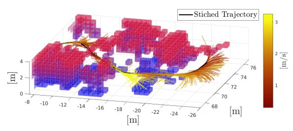
the quadrotor. In [3], it was shown that with continuous minimum-jerk trajectories and fast re-
planning, they achieved higher trajectory smoothness compared to other, more reactive planners.
Figure 2.3 shows the smooth trajectory generated by tracking motion primitive-generated paths.
Gao, et al. (2018) [19] first finds a time-indexed minimal arrival path that may not be feasible for
quadrotor flight, and then forms a surrounding free-space flight corridor in which they generate
a feasible trajectory. They use a Bernstein polynomial basis and represent the trajectory as a
piecewise Bézier curve.
Figure 2.3: Example of concatenated trajectories in a cluttered environment. Colored lines represent individual motion
primitives; the quadrotor tracks the initial part of every generated trajectory, forming a complete, stitched trajectory
represented by the black line. [3]
To follow trajectories, controllers take in a desired trajectory typically composed of position way-
points each with an associated velocity, and issue actuator commands to the robot. In the MAV
case, an autopilot software may accept attitude or attitude-rate commands which come from such a
controller. Hoffman, et al. (2008) [20] demonstrated a controller that took as input a non-feasible
trajectory and outputted feasible attitude commands for a quadrotor that accurately followed the
original path. This was demonstrated outdoors with 50cm accuracy. A similar approach was taken
(but extended to 3D) for the path following controller implemented in [21]. Here, the desired po-
sition and desired velocity from the closest point on the trajectory are used to find the position and
velocity errors of the robot. These are used to calculate the desired robot acceleration with PD
feedback and a feedforward term.
78
Chapter 3

Targeting Moving Objects with a Quadrotor

As described in Section 2.1, servoing towards moving targets is challenging with classical methods.
As such, LOS-based guidance principals (Section 2.2) and trajectory following methods (2.3) may
produce better results when target acceleration is nonzero. In addition, the quadrotor platform’s
control limits might be avoided with smooth trajectory-based methods. This chapter focuses on the
development and evaluation of various such guidance methods to achieve impact with a generalized
form of an aerial, mobile target. No information is known about the target other than its color,
which is used for segmentation in an RGB image to simplify the detection and tracking problem.

3.1     Line-of-Sight Guidance
3.1.1    Derivation of True Proportional Navigation Guidance Law
Line-of-sight (LOS) guidance methods are used to apply acceleration commands to the pursuer that
minimize change in the LOS vector towards the target. In this section, the basic LOS geometry is
introduced and used to derive proportional navigation (PN) guidance. Following subsections show
how this is used, with target detections, to calculate quantities used for the applied PN guidance.
As seen in Figure 3.1, the fixed world coordinate frame is specified by the unit vectors 1̄x , 1̄y , 1̄z .
The LOS coordinate frame, attached to the moving missile, is specified by the unit vectors 1̄r , 1̄n ,
1̄ω ; 1̄r points along the LOS r̄; 1̄n is the change in direction (i.e. a rotation) of the LOS vector; 1̄ω
is the cross product of the former two, in that order (forming a right-handed coordinate frame).
In general, the angular velocity of the LOS coordinate frame is given by:

                                      φ̇¯ = Φ̇r 1̄r + Φ̇n 1̄n + Φ̇ω 1̄ω                             (3.1)

Where Φ̇r , Φ̇n , Φ̇ω are the magnitudes of the components of the angular velocity defined as:

                                                     9
Figure 3.1: LOS coordinate system [4].
Φ̇r = φ̇¯ • 1̄r (3.2)
Φ̇ = φ̇¯ • 1̄
n n (3.3)
Φ̇ω = φ̇¯ • 1̄ω (3.4)
As derived in [4] but not reproduced here, the components of the relative acceleration between the
missile and target are:
(āT − āM ) • 1̄r = R̈ − RΦ̇2ω (3.5)
(āT − āM ) • 1̄n = 2ṘΦ̇ω + RΦ̈ω (3.6)
(āT − āM ) • 1̄ω = RΦ̇ω Φ̇r (3.7)
Where āT and āM are the target and missile accelerations, respectively. From this result, specifi-
cally using the condition in Equation 3.5, we can list sufficient conditions to satisfy the equation
and ensure intercept: (i) interceptor is able to achieve an acceleration along the LOS greater than
that of the target ((āT − āM ) • 1̄r < 0), (ii) the initial rate of change in the range R is negative
(Ṙ < 0), which then ensures R̈ < 0 given the first condition, and (iii) the rate of change in the
LOS is 0 (Φ̇ω = 0). Condition (i) depends on the nature of the interceptor and target; condition (ii)
implies that PN pursuit must be initialized with a positive closing velocity; condition (iii) implies
10that the interceptor must satisfy acceleration commands such that the LOS vector remains constant.
Palumbo, et al. (2010) finds the following true PN (TPN) law that ensures system stability:
āM • 1̄n = N Vc Φ̇ω , N > 2 (3.8)
Where N is a proportional gain and Vc is the closing velocity. In other words, the interceptor
acceleration āM must have a component, orthogonal to the LOS, proportional to the rotation rate
of the LOS as specified in Equation 3.11.
3.1.2 True Proportional Navigation
To generate the desired acceleration vector with magnitude specified by Equation 3.8 and direction
orthogonal to the LOS, we first calculate both Φ̇ω (directly represented in Equation 3.8) and 1n
(acceleration direction). The target’s centroid in image frame coordinates at times t − 1 and t is
represented by (ut−1 , vt−1 ) and (ut , vt ), respectively, as shown in Figure 3.2. The camera principal
point, specified in the calibrated camera’s intrinsic matrix (typically denoted K), is represented by
(cx , cy ).
Figure 3.2: Example image frame with de-
tected object’s centroid at times t − 1 and t.
Figure 3.3: Top-down diagram showing intermediate quantities in cal-
culation of desired acceleration command.
The LOS vector rt in the camera’s frame of reference at time t is given by the following.
ut − cx
fx
vt − cy
rt = (3.9)
fy
1
11In the special case of the first iteration of the algorithm, at t = 0, the LOS vector is calculated
according to Equation 3.9 then stored for use as rt−1 the upcoming iteration. For the t = 0
computation cycle the control output is set to 0.
The angle spanned by the two vectors rt and rt−1 is as follows:
< rt , rt−1 >
Φω = arccos (3.10)
||rt ||||rt−1 ||
Therefore, if the difference in time for one cycle is represented by ∆t, then the magnitude of the
rotation rate of the LOS vector is:
Φω
Φ̇ω = (3.11)
∆t
The direction of the acceleration (direction of the LOS rotation) 1n is shown in Figure 3.3 and
calculated below.
n = rt − proj(rt , rt−1 ) (3.12)
rt−1 rt−1
= rt − < rt , > (3.13)
||rt || ||rt ||
n
1n = (3.14)
||n||
Where the vector projection of rt onto rt−1 is represented by the red vector in Figure 3.3. With the
scalar Φ̇ω and the vector 1n , we can compute the desired acceleration as follows.
aLOS 0 = N Vc Φ̇ω 1n (3.15)
In application on a quadrotor, in this work, the acceleration vector is fed into a velocity controller
by integration of the command, which submits a roll, pitch, yawrate, thrust command to the internal
autopilot controllers. Therefore, rather than adjusting heading to satisfy lateral accelerations, the
application of TPN in this work relies on roll angle control. This more direct method of achieving
lateral accelerations (that does not require forward velocity) is not possible on a missile or fixed-
wing aircraft.
3.1.3 Proportional Navigation with Heading Control
The TPN algorithm presented above maintains the integrity of the algorithm commonly presented
in missile guidance literature, but applies the control command more directly by controlling the
roll angle of the UAV. During a missile’s flight, the vehicle fulfills desired acceleration commands
by flying in an arc, gradually changing its heading by relying on forward motion and the use of
12thrust vectoring or control surfaces. A quadrotor, however, has direct control over its heading by
applying yaw-rate control. In this section, we describe an algorithm that uses PN acceleration in
all axes but the lateral axis, and instead controls the heading to achieve lateral acceleration. Since
it does not utilize PN in the lateral axis, we do not assign the label of “true”.
We define an inertial reference frame at the center of the UAV, with x pointing forward, y pointing
to the left, and z point upward. The acceleration along the x and z axes are simply taken from
Equation 3.15 as the corresponding components:
ax = aLOS 0 • 1x (3.16)
az = aLOS 0 • 1z (3.17)
The heading control composes of a commanded yaw-rate, which includes the computation of the
heading:
yaw
˙ = KP,yaw heading (3.18)
r t • 1y
= KP,yaw arctan (3.19)
rt • 1x
Where KP,yaw is a tuned proportional gain and rt is the current LOS vector.
3.1.4 Hybrid TPN-Heading Control
There are potential benefits to both methods presented in Sections 3.1.2 and 3.1.3. TPN specifically
applied to quadrotors via roll angle control might yield quicker reaction time for a moving object.
PN while keeping the target centered in the frame ensures that the target is not lost from frame;
otherwise, in a full system, the pursuing UAV would have to return to a search pattern. The goal
of the hybrid algorithm is to capture the advantages of both methods.
This method switches between the two modes, PN and Heading. The transition between them
simply relies on a tuned threshold kheading on the heading towards the target.
If |heading| < kheading , enter state PN:
ax = aLOS 0 • 1x (3.20)
ay = aLOS 0 • 1y (3.21)
az = aLOS 0 • 1z (3.22)
yaw
˙ = 0.2KP,yaw heading (3.23)
13If |heading| ≥ kheading , enter state Heading Control:
ax = aLOS 0 • 1x (3.24)
ay = 0.2aLOS 0 • 1y (3.25)
az =0 (3.26)
yaw
˙ = KP,yaw heading (3.27)
Where kheading may be tuned depending on certain factors of the UAV system, including the camera
field-of-view (FOV) or the maximum yaw-rate. Note that at all times, regardless of the heading,
both ay and yaw˙ are nonzero, and are instead suppressed with a factor less than 1. The factor of
0.2 was found empirically in this study to perform well and yield an appropriate influence of both
acceleration and yaw-rate. Using this hybrid method, the UAV may potentially be able to react to
changes in target motion while also keeping it in view.
3.2 Trajectory Following
Figure 3.4: Diagram of trajectory replanning by stitching trajectory to the look ahead point. UAV closely follows the
tracking point.
All trajectory following methods were implemented with some replanning rate at which updated
trajectories are published. Replanning is constantly done from the look ahead point, which is
maintained by the Trajectory Controller as described in Section 3.3.2.
3.2.1 LOS 0 Acceleration Trajectory Following
These trajectories are formed by taking the desired acceleration command calculated with Equation
3.15 and calculating position waypoints and velocities given the starting position set to the look
ahead point. The calculations for the positions and velocities are done with the following kinematic
equations, set in the UAV’s inertial reference frame.
141
pt = v0 t + aLOS 0 t2 (3.28)
2
vt = v0 + aLOS 0 t, t = 0, 0.1, ..., T (3.29)
Where T is the time length of each trajectory. As T approaches 0, this method becomes equivalent
to commanding the desired LOS 0 acceleration directly. The discretization of the timesteps is also
a tunable parameter.
3.2.2 Target Motion Forecasting
In its simplest form, target motion forecasting involves estimating the target velocity in 3D, calcu-
lating the future location of the target with a straight-line path, and generating a collision course
trajectory towards that point in space at a velocity which completes the trajectory at the specified
time. This method makes three critical assumptions: (i) the target has zero acceleration, (ii) we can
approximate time-to-collision by calculating the time along the current LOS vector, and (iii) the
forecasted target position will change slowly, so generating straight-path trajectories is sufficient to
result in a final, smooth stitched trajectory. First, the LOS unit vectors at two times are calculated.
These are used along with the depth estimation to find the target’s velocity:
d1 (1LOS1 ) − d0 (1LOS0 )
vtarget = (3.30)
t1 − t0
d1 and d0 , 1LOS1 and 1LOS0 , and t1 and t0 are the estimated depth, calculated LOS unit vector, and
time, at two timesteps. Once we have the velocity, we find the approximate time-to-collision along
the current LOS vector by using the UAV’s velocity component along the LOS:
d1
tcollision = (3.31)
< vU AV , 1LOS1 >
Where vU AV is the current UAV velocity vector. Therefore, the approximate point in space to plan
the trajectory to is as follows, where pcollision is in the UAV reference frame.
pcollision = vtarget tcollision + d1 (1LOS1 ) (3.32)
3.3 System
Figure 3.5 shows a diagram of the most important parts of the system, including perception, con-
trol, and the simulation software. Each block generally consists of one or two nodes in ROS (Robot
Operation System), the framework used in this work.
15Figure 3.5: System diagram.
3.3.1 Perception
Object Segmentation
(a) RGB image frame with target in view during (b) Binary segmentation image with target high-
pursuit. lighted.
Figure 3.6: Input and output of Object Segmentation node.
Since the focus for this chapter was on the comparison of guidance methods, the perception chal-
lenge was simplified. The simulation does not include rich background visuals, there is no dropout
in the camera feed, and the object was reduced from a potential UAV shape to a yellow sphere. The
segmentation node composes of color thresholding that creates a binary segmentation image from
16each camera frame in real-time (30Hz), as seen in Figure 3.6b. In addition, this node publishes the
centroid (Cx , Cy ) of the detected object by using the image moments.
M10
Cx M
00
= (3.33)
Cy M
01
M00
Object Depth Estimation
Figure 3.7: Example image frame with detected ob-
ject’s centroid and part of depth estimation calculations.
(ulef t , vlef t ) and (uright , vright ) points along image hori-Figure 3.8: Top-down diagram showing calculation of es-
zontal corresponding to target edges are shown before (red)timated distance to object center d0 with 3D projected rays
and after (black) rotation back into the original segmentedto target edges.
coordinates. Note that because of the wide field of view,
images around the edges of the image frame can get warped
even though there is no distortion in this camera model.
Depth estimation with monocular camera images relies on prior knowledge of the target size as well
as the assumption that the target is spherical (which is correct in this simulation, but extendable
to real-life targets with approximate knowledge of target or aircraft type). The estimate takes
into account the camera intrinsic parameters and projects the 2D information (pixels) to 3D (rays
starting at the camera center) to extract the depth.
Pixel coordinates at two points in the image need to be located which form a 2D line in the image
that projects to a 3D line along the diameter of the object. The easiest found such line is the line
through the image principal point that passes through the centroid, since the target is a sphere.
This line is the dotted line passing through the target in Figure 3.7. We must first find the pixel
coordinates along this line that correspond to the object edges in the image.
First, we find the rotation angle formed by the centroid coordinates with respect to the image
horizontal, labeled θ in Figure 3.7.
17C y − cy
θ = arctan (3.34)
C x − cx
With this angle we can use a rotation matrix to rotate the segmented object onto the y = cy line.
Note that we use −θ to achieve the correct rotation, and that we first compute new pixel coordinates
(ui , vi ) relative to the image center, from the original coordinates (xi , yi ).
ui x i − cx
= , i = 1, ..., N (3.35)
vi y i − cy
ui,R cos(−θ) −sin(−θ) ui
= , i = 1, ..., N (3.36)
vi,R sin(−θ) cos(−θ) vi
Where N is the total number of segmented pixels in the binary segmentation image. Once the
object is rotated onto the image horizontal, simple min and max operations yield the extreme
pixel coordinates on the left and right of the target (or right and left, if Cx < cx ).
ulef t mini (ui )
= , i = 1, ..., N (3.37)
vlef t cy
uright maxi (ui )
= , i = 1, ..., N (3.38)
vright cy
These two points are shown in red in Figure 3.7. We apply the inverse rotation and translation to
get the original coordinates of these two identified pixel coordinates.
ulef t,R−1 cos(θ) −sin(θ) ulef t c
= + x (3.39)
vlef t,R−1 sin(θ) cos(θ) vlef t cy
uright,R−1 cos(θ) −sin(θ) uright c
= + x (3.40)
vright,R−1 sin(θ) cos(θ) vright cy
These two pixels are projected to 3D rays similar to the LOS ray calculation in Equation 3.9. They
can also be seen in a similar top-down view in Figure 3.8. Once the two rays are found, the depth
(to the nearest point on the object) is as follows:
w/2 w
d= − (3.41)
sin (α/2) 2
18LOS and LOS 0 Computation
The calculation of rt , the LOS vector, can be found in Equation 3.9. The calculations of Φ̇ω and 1n ,
the scaling and directional components of LOS’, can be found in Equations 3.11 and 3.14. Before
being input to the Guidance node, the quantities undergo smoothing with a flat moving average
filter. The filtered values are used for trajectory-based guidance, while LOS-based guidance uses
the raw values.
3.3.2 Control
Guidance
The Guidance node either executes LOS-based or trajectory-based guidance. The LOS-based guid-
ance, as described in Section 3.1, utilizes the LOS and LOS’ computation from the Perception
block. In this case, the node outputs acceleration commands that are satisfied by the Velocity
Controller. Trajectory-based guidance utilizes both the LOS information as well as the depth esti-
mate to generate 3D trajectories towards the target’s current state or forecasted motion. Here, the
node outputs a trajectory composing of waypoints and corresponding speeds which is accepted by
the Trajectory Controller. Every method is initialized with two seconds of simple LOS guidance,
where the UAV accepts velocity commands directly along the current LOS vector.
Trajectory, Pose, and Velocity Controllers
The Trajectory Controller accepts a trajectory in the form of a list of waypoints, each with a cor-
responding (x, y, z) position, yaw, and speed (scalar). It outputs a tracking point, which the Pose
Controller takes as input for tracking the trajectory, and a look ahead point, which is used as the
replanning point. The configurable look ahead time sets how far ahead the look ahead point is
from the tracking point, and is approximated to be 1/f + ∆buf f er, where f is the replanning
frequency and ∆buf f er is a buffer in case there is some lag in the system. The Pose Controller
composes of PID controllers with the tracking point from the Trajectory Controller as the reference
and the odometry from the PX4 SITL interface as the actual. This outputs a velocity reference (and
a velocity feedforward term from the Trajectory Controller) to the Velocity Controller, which also
accepts the odometry from the PX4 SITL interface as the actual. The Velocity Controller also uses
PID controllers, and outputs a roll, pitch, yawrate, thrust commands to the PX4 SITL interface.
3.3.3 Simulation Package
Gazebo and PX4 SITL
Simulation was used to develop, deploy, and evaluate many UAV guidance algorithms quickly. In
this environment, the behavior of the UAV and the target was easily modified and could be strained
without the safety risk involved in real-world testing. Gazebo [22], the simulator of choice, is
commonly used for robotics testing and simulates robot dynamics with the ODE physics engine.
This was paired with PX4 autopilot [23] software-in-the-loop (SITL) for control of the quadrotor.
19Figure 3.9: Gazebo simulation world, with UAV model and target in view.
An example of the simulated world can be seen in Figure 3.9. Obstacles, a visually rich backdrop,
and other factors were eliminated in the simulation setup to reduce the impact of external factors
on the evaluation of the guidance algorithms. When deployed on a real-world UAS, the algorithms
here can be merged within a larger autonomy architecture including robust detection and tracking,
as well as obstacle avoidance and others. The quadrotor is outfitted with a RGB camera that models
a realistic vision sensor.
Target Position Controller
(a) Straight target path. (b) Figure-8 target path. (c) Knot target path.
Figure 3.10: Target path library taken from similar perspectives. Dark blue sphere is the target’s current position.
Light blue sequence is the traced path. (a) straight path with random slope; (b) figure-8 path with random tilt, of size
10m×6m; (c) knot path with random center point, of size 2m×2m×2m.
A library of target paths was used to strain the UAV’s capability of intercepting the target. The first,
simplest target motion is a straight path with constant velocity, which may mimic an autonomous
aircraft on a search pattern or a fixed-wing plane. The starting position places the target on either
side of the UAV’s FOV, and the path crosses in front of the UAV with some random variation in
slope. The third trajectory is a figure-8 with a randomized 3D tilt, similar to an evasive maneuver
20a small aircraft may take. These trajectories can be seen in Figure 3.10. The third trajectory com-
poses of a knot shape filling a 2m×2m×2m space at a random location within a 10m×20m×10m
area in front of the UAV. This more rapid movement back and forth is similar to a multi-rotor
hovering in a changing wind field.
3.4 Results
In this section, we evaluate the five guidance algorithms described in the sections prior (Sections
3.1.2, 3.1.3, 3.1.4, 3.2.1, 3.2.2). An experiment configuration composed of a selection of one
parameter from each of the following categories. Each configuration underwent 50 trials.
UAV Guidance: True Proportional Navigation (TPN), Proportional Navigation with Head-
ing Control (PN-Heading), Hybrid True Proportional Navigation with Heading Control (Hy-
brid TPN-Heading), LOS’ Trajectory, Forecasting Trajectory
UAV speed [m/s]: 2.0, 3.0, 4.0, 5.0
Target path: Straight, Figure-8, Knot
Target speed [% of UAV speed]: 25%, 50%, 75%, 100%
In the case of sinusoidal target paths (figure-8 and knot), the target speed was set by determining
the length of the path and dividing by the desired speed to calculate the period of the sinusoids.
The primary metric for comparing different methods is the first-pass hit rate, presented in Section
3.4.1. All of the following conditions must be met for a trial to be considered a successful first-pass
hit on the target.
1. UAV is within 0.5m of the target (measured from the closest point on the target to the center
of the UAV).
2. Duration of pursuit is less than 20s.
3. UAV stays within a 35m×100m×40m area surrounding the target.
4. Target is not outside the UAV camera’s FOV for more than 3s.
These conditions were specified after consideration of the simulation scene, UAV model, and target
model. The target is a yellow sphere of diameter 1m. The RGB camera has a horizontal FOV of
105◦ with a size 680×480. In lieu of a gimbal camera in simulation, the UAV model had a rigidly
fixed, angled camera that was adjusted for each speed, to compensate for the steady state pitch
down when flying forward at high speeds.
The next metric presented is the mean pursuit durations, in Section 3.4.2. These were computed
by taking the mean of the time-to-hit measurements over each of (a) target speed, and (b) UAV
velocity, respectively. This was done using only the successful hits during each experiment.
213.4.1 First-Pass Hit Rates
Datapoints in the following heatmaps that are inside a black square represent experiments that were
not able to complete more than 95% of the trials without crashing due to UAV instability with the
particular experiment configuration.
(a) Straight target path. (b) Figure-8 target path. (c) Knot target path.
Figure 3.11: True Proportional Navigation hit rate across three target paths.
(a) Straight target path. (b) Figure-8 target path. (c) Knot target path.
Figure 3.12: Proportional Navigation with Heading Control hit rate across three target paths.
TPN achieves the highest hit rate across almost all configurations compared to the other methods
in both classes (LOS Guidance and Trajectory Following). Across all experiments there is a trend
of lower UAV and target speeds resulting in higher hit rates, sometimes even of 1.0 (i.e., 50 of 50
trials result in a hit). Moving down and to the right within each subfigure presents results at higher
target and UAV speeds. This can be seen as increasing the closing velocity, which reduces the time
that the UAV has to react to changes in target motion. As seen in the figures, this results in lower
hit rates, which may be due to lag in the UAV controllers’ ability to fulfill desired acceleration
22(a) Straight target path. (b) Figure-8 target path. (c) Knot target path.
Figure 3.13: Hybrid True Proportional Navigation-Heading Control hit rate across three target paths.
(a) Straight target path. (b) Figure-8 target path. (c) Knot target path.
Figure 3.14: LOS’ Trajectory hit rate across three target paths.
commands. The quadorotor achieves a lateral acceleration more directly than a fixed-wing craft
by inducing a roll angle and thereby shifting a component of the thrust to this axis. However, the
moment of the aircraft and the response time of the controller both contribute to lag in achieving the
necessary roll angle. Therefore, as the time allowed for this control decreases, with the increase in
closing velocity, it is more unlikely that the necessary lateral acceleration will be achieved. Similar
logic applies to the thrust controller for achieving desired acceleration in the z axis. It is possible
that a more accurate controller might increase the hit rates at high closing velocities.
The Hybrid TPN-Heading method generally had higher hit rates than PN-Heading, but lower than
TPN. However, Hybrid TPN-Heading consistently performed better than TPN at a low target speed
(25%) in the straight and figure-8 target path, with the highest increase in hit rate as 0.28 among
these configurations. This suggests that similar to the behavior of PN-Heading at low target speeds
(further described in a below section), Hybrid TPN-Heading is able to chase the target at these
23(a) Straight target path. (b) Figure-8 target path. (c) Knot target path.
Figure 3.15: Forecasting Trajectory hit rate across three target paths.
speeds even if the initial TPN-driven approach is unsuccessful.
The LOS Guidance class of methods generally has higher hit rates than the Trajectory Follow-
ing methods implemented here. When designing these algorithms and implementing them, it was
found that significant parameter tuning and filtering was necessary to improve the results of the Tra-
jectory Following methods. For example, although the LOS’ Trajectory method produces smooth
trajectories and therefore smoother UAV flight, it has to use a filtered (smoothed with flat moving
average filter) LOS’ in order to create consistent trajectories. This filtering introduces lag, which
quickly becomes intractable when the target or UAV speed is increased past what was used for
tuning the system. This is amplified in the case of the Forecasting Trajectory. While Equation
3.32 is geometrically sound, in the simulated system imperfections in depth estimation, LOS com-
putation, and corresponding frame transformations (especially during high roll- and pitch-rates)
cause inaccuracies that require filtering and tuning to make the 3D target forecast feasible. These
limitations are largely a byproduct of using only monocular camera information to estimate 3D
positioning. The effect can be seen in the UAV instability in the majority of experiments shown in
Figure 3.15.
TPN with Straight Target Path at Low Speeds
While TPN generally achieves the highest hit rate compared to all other methods presented here,
a notable exception is the slowest configuration of UAV velocity 2m/s and target speed 25% with
the straight target path, which has a hit rate of 0.48. Figure 3.16 shows that the target progressively
gets farther out of view as the UAV flies by. The straight target path begins on one side of the
pre-defined arena space and terminates on the other side, with randomized variation in path slope.
Since the target moves so slowly in this configuration, it remains on one side of the UAV’s image.
The y component of the body-frame acceleration command generated by TPN while the target is
moving towards the edge of the image (due to the UAV’s forward velocity) is not enough to keep
the target in sight, and it slowly slips out of view. This problem becomes less likely at higher
24UAV speeds, however, since the greater motion of the UAV creates more motion of the target in
the image, thereby creating a larger lateral acceleration command that keeps the target in view.
This issue is only apparent in the straight path case since only with this path the starting target
location had to be on the edges of the image to compensate for larger movement at higher target
speeds. This issue does not appear in the PN-Heading or Hybrid TPN-Heading methods, since
they compensate by commanding yaw-rate to center the object in the image.
25(a) Top-down view of UAV (RGB axes) ap- (b) Capture of image frame from UAV camera at
proaching target (blue). Paths shown are ap- the point shown in 3.16a.
proximately 5 seconds in length, with UAV path
continuing off-screen.
(c) Top-down view approximately 2s after (d) Capture of image frame from UAV camera at
3.16a. the point shown in 3.16c.
(e) Top-down view approximately 2s after (f) Capture of image frame from UAV camera at the
3.16c. point shown in 3.16e.
Figure 3.16: Demonstration of TPN, straight target path, UAV speed 2m/s and target speed 25% (0.5m/s); correspond-
ing datapoint is represented in top left corner of Figure 3.11a.
26PN-Heading at High Speeds
PN-Heading has lower performance at high UAV or target speeds relative to both TPN or Hybrid
TPN-Heading. This was often observed to be due to the time required to effectively change the
UAV’s velocity direction through a yaw-rate, and this time delay increases further as the UAV
speed increases. A notable artifact in the results can be seen in Figure 3.12a, where the results at
100% target speed is 0 at every UAV velocity. This is due to the way in which the UAV “chases”
the target in the straight target path scenario. Figure 3.21 shows that the UAV might pass the
target initially, but turns towards it via commanding a yawrate, and finds it again (within the 3s
detection timeout). Then it is able to pursue the target with PN acceleration commands in the x
and z directions. However, during this chase period, the UAV’s velocity is in the same direction
as the target’s. Therefore, the target’s speed must be less than the UAV’s, or it will be impossible
to maintain a nonzero closing velocity. This is the case specifically for the bottom row of Figure
3.12a. This does not occur with the other target motions since the target has non-zero acceleration.
3.4.2 Pursuit Duration
If there were no hits across all experiments for a particular configuration, then those data points
are missing in the figures, as seen in 3.17a and 3.17b.
(a) Pursuit duration vs. UAV velocity. (b) Pursuit duration vs. target speed.
Figure 3.17: Mean pursuit durations for straight target path.
27(a) Pursuit duration vs. UAV velocity. (b) Pursuit duration vs. target speed.
Figure 3.18: Mean pursuit durations for figure-8 target path.
(a) Pursuit duration vs. UAV velocity. (b) Pursuit duration vs. target speed.
Figure 3.19: Mean pursuit durations for knot target path.
The pursuit times generally decreased as UAV velocity increased, though this trend is not as appar-
ent in some of the guidance methods in Figure 3.17a. In the straight target path scenario, because
the target has constant velocity it will eventually be out of the UAV’s FOV, restricting the time
window in which an intercept is possible. A strong downward trend is still apparent with TPN and
PN-Heading.
28The effect of target speed on pursuit duration is most observed in the straight target path case. Here,
the increase in target speed caused increased times for PN-Heading and Hybrid TPN-Heading.
Both of these methods utilize yaw-rate control to keep the target centered in the UAV’s camera
image, and as shown in Figure 3.21, this can result in the UAV turning and “chasing” the target as
it passes. As the target speed increases, the probability of a successful hit on first approach goes
down, which then increases the chance of this kind of chasing maneuver.
LOS’ Trajectory, though using a smoothed version of the LOS’ used for TPN, does not exhibit
as strong of a decrease in pursuit time over increasing UAV velocity or target speed. These re-
sults actually show that of all methods, LOS’ Trajectory has the lowest pursuit durations with few
exceptions. However, when paired with the results in Figure 3.14, it seems more likely that these
times are a byproduct of being most likely to hit a target that is initialized closer to the UAV starting
point.
3.4.3 Pursuit Behavior
In this section, we present each method’s UAV path relative to target motion in hand-picked con-
figurations for qualitative assessment.
Figure 3.20: TPN behavior.
29Figure 3.21: PN-Heading behavior.
Figure 3.22: Hybrid TPN-Heading behavior.
30Figure 3.23: LOS’ Trajectory behavior.
Figure 3.24: Forecasting Trajectory behavior.
Figure 3.20 shows the UAV track the target’s motion as it dips and then rises again as it moves
through one half of the figure-8 path. Figure 3.21 shows the UAV approach the straight target path
but make a sharp left turn via yaw-rate commands as it passes by. It then goes on to implement PN
to catch the target. Figure 3.22 starts with motion similar to TPN, then uses heading control to yaw
towards the target when it is close and the heading becomes larger. Figure 3.23 shows a smoother
path than TPN, as a result of smoothing the PN commands and utilizing trajectory following. The
trajectory generated at the timestamp shown in the image is shown in yellow. Figure 3.24 shows
the path mimicking the motion of the target, but shifted in space due to forecasting of the target
motion. The current forecasted trajectory is shown in yellow.
3132
Chapter 4
LOS Guidance Applied in a Robotics
Competition Setting
4.1 Introduction
The Mohamed Bin Zayed International Robotics Challenge 2020 is an outdoor robotics competi-
tion in which dozens of international teams, including many top robotics universities, demonstrate
autonomous performance in different tasks.
“MBZIRC aims to provide an ambitious, science-based, and technologically demand-
ing set of challenges in robotics, open to a large number of international teams. It is
intended to demonstrate the current state of the art in robotics in terms of scientific and
technological accomplishments, and to inspire the future of robotics.” [24]
Teams had the choice of competing in any or all of three challenges, differentiated by the types
and number of robots allowed, the theme of the tasks involved, and physically separated arenas.
Challenge 1: Airspace Safety involved aerial robots targeting semi-stationary and moving targets;
Challenge 2: Construction involved both ground and aerial robots building separate wall structures
with provided blocks of varying size and weight; Challenge 3: Firefighting involved ground and
aerial robots cooperating to extinguish real and fake fires surrounding and inside a three-story
building. The work towards competing in Challenge 1 and the associated competition results are
the most relevant towards the thesis of airspace safety, and are therefore the focus in this report.
In Challenge 1, the two primary tasks are as follows:
Task 1: Semi-stationary targets. Pop five 60cm-diameter green balloons placed randomly
throughout the arena.
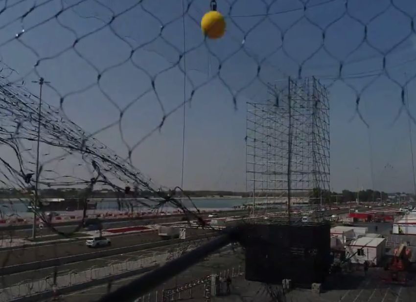
Task 2: Moving target. Capture and return a 15cm yellow foam ball hanging from a UAV
flying throughout the arena in a figure-8 path.
The balloons were placed on rigid poles but filled with helium and attached to the pole with string;
33You can also read