Retrieval of total water vapour in the Arctic using microwave humidity sounders - Atmos. Meas. Tech
←
→
Page content transcription
If your browser does not render page correctly, please read the page content below
Atmos. Meas. Tech., 11, 2067–2084, 2018
https://doi.org/10.5194/amt-11-2067-2018
© Author(s) 2018. This work is distributed under
the Creative Commons Attribution 4.0 License.

Retrieval of total water vapour in the Arctic using microwave
humidity sounders
Raul Cristian Scarlat, Christian Melsheimer, and Georg Heygster
Institute of Environmental Physics, University of Bremen, Bremen, Germany

Correspondence: Raul Cristian Scarlat (rauls@iup.physik.uni-bremen.de)

Received: 6 July 2017 – Discussion started: 3 November 2017
Revised: 27 February 2018 – Accepted: 8 March 2018 – Published: 11 April 2018

Abstract. Quantitative retrievals of atmospheric water             tent of air is regulated through the processes of condensa-
vapour in the Arctic present numerous challenges because           tion, evaporation and, since the advent of life on this planet,
of the particular climate characteristics of this area. Here, we   transpiration. These phase changes provide the mechanisms
attempt to build upon the work of Melsheimer and Heyg-             through which water vapour influences atmospheric temper-
ster (2008) to retrieve total atmospheric water vapour (TWV)       ature by adding or removing energy from the air. Through
in the Arctic from satellite microwave radiometers. While          evaporation, energy is stored as latent heat within the wa-
the above-mentioned algorithm deals primarily with the ice-        ter molecules that break away from the liquid as gas, thus
covered central Arctic, with this work we aim to extend the        leading to a cooling effect in its immediate vicinity. The re-
coverage to partially ice-covered and ice-free areas. By us-       verse of this process releases this latent heat through con-
ing modelled values for the microwave emissivity of the ice-       densation and provides energy, e.g. for the development of
free sea surface, we develop two sub-algorithms using dif-         thunderstorm cells.
ferent sets of channels that deal solely with open-ocean ar-          One of the main characteristics of atmospheric water
eas. The new algorithm extends the spatial coverage of the         vapour is its high variability (Trenberth et al., 2005), both
retrieval throughout the year but especially in the warmer         in terms of spatial location and temporal evolution. Because
months when higher TWV values are frequent. The high               of this variability water vapour can be used as an atmo-
TWV measurements over both sea-ice and open-water sur-             spheric tracer that indicates general atmospheric circulation
faces are, however, connected to larger uncertainties as the       as it accompanies the horizontally moving air masses, while
retrieval values are close to the instrument saturation limits.    its phase changes indicate the location of upwelling or down-
   This approach allows us to apply the algorithm to regions       welling currents. The average lifetime of a molecule of wa-
where previously no data were available and ensures a more         ter in the atmosphere is 10–12 days, during which it can go
consistent physical analysis of the satellite measurements by      through many phase changes.
taking into account the contribution of the surface emissivity        Water vapour is one of the major greenhouse gases in the
to the measured signal.                                            atmosphere. As such, it is important to monitor the vari-
                                                                   ability of water vapour considering the anthropogenic in-
                                                                   crease of other greenhouse gases (Solomon et al., 2010).
                                                                   In the context of global warming the atmosphere’s load ca-
1   Introduction                                                   pacity for water vapour increases and therefore its contribu-
                                                                   tion as the most important greenhouse effect warrants pre-
Water vapour plays a crucial role within the complex sys-          cise monitoring. Model data indicate that this positive feed-
tem of our atmosphere. It transports energy from the warmer        back loop would increase the sensitivity of surface tem-
lower latitudes to higher ones, influencing global weather         peratures to carbon dioxide concentrations by a factor of
patterns, plays a significant part in trapping infrared (IR) ra-   2 (Held and Soden, 2000) without taking into consideration
diation, and is highly variable throughout the planetary at-       other possible feedback processes. However, this matter is
mosphere (Le and Gallus Jr., 2012). The water vapour con-

Published by Copernicus Publications on behalf of the European Geosciences Union.
2068                                                        R. C. Scarlat et al.: Retrieval of total water vapour in the Arctic

still debated, as the atmospheric storage of water vapour          central Arctic region for most of the year and it shows good
is not understood well enough to warrant definitive con-           agreement with retrievals based on the analysis of GPS sig-
clusions. Its importance as a greenhouse gas and the posi-         nals taken at stations around Antarctica (Vey et al., 2004).
tive feedback loop associated with atmospheric water vapour        However, because of the limited TWV retrieval range, this
make it necessary to have accurate global scale data on this       method alone cannot ensure year-long monitoring of TWV
parameter.                                                         values (Selbach et al., 2003).
   For the purpose of taking measurements, we quantify the            The Antarctic algorithm (Miao et al., 2001) worked inde-
atmospheric water vapour load as a vertically integrated mass      pendently of the surface type by assuming the same surface
over a column of air with a base area of 1 m2 and name it total    emissivity for all channel frequencies used. While this is a
water vapour or TWV for short. It is the parameter that we         valid assumption for the case in which the three 183.31 GHz
will be discussing throughout this paper when referring to         band channels are used, as the surface emissivities are very
measured atmospheric water vapour content.                         close to each other, it is a poor assumption when using a
   A reliable method used to retrieve atmospheric water            triplet that includes the 150 GHz channel (Wang et al., 2001),
vapour content is by using balloon-borne radiosondes. This         which has a different surface emissivity from the 183.31 GHz
is an accurate method which provides good vertically re-           bands. The emerging errors from the emissivity differences
solved measurements. However, these are only point mea-            were deemed acceptable as a trade-off for extending the re-
surements and thus only of local significance (Hurst et al.,       trieval range from 1.5 to 2 kg m−2 (when using all three
2011). Ground-based retrievals such as fixed radiometers and       band channels) up to 7 kg m−2 (when using the 183.31 ± 3
GPS-based retrievals achieve a lower vertical resolution but       and 183.31 ± 7 GHz together with the 150 GHz channel). To
are considered feasible for monitoring purposes in regions         improve on this performance the algorithm developed by
with a high density of ground stations (Das et al., 2014).         Melsheimer and Heygster (2008) extends the TWV retrieval
However, only satellite measurements fulfil the global cov-        range over sea ice by including the 89 GHz channel into the
erage requirements of modern numerical weather prediction.         retrieval. Using the triplet of 183.31 ± 7, 150 and the 89 GHz
Because of the strong absorption properties of water vapour        channels allows the retrieval to function up to the saturation
in the infrared and microwave range, suitable space-borne          limit of the 183.31 ± 7 GHz channel.
instruments can ensure a complete global coverage of wa-              By using the 89 GHz channel, the difference in surface
ter vapour retrievals (Miao, 1998; Szczodrak et al., 2005;         emissivity for the different frequencies becomes too great
Bobylev et al., 2010).                                             and the equal emissivity assumption has to be dropped. In
   Radiosonde retrieval of total water vapour in the Arctic        order to increase the retrieval range, some information about
is not sufficient because of the scarcity of weather stations      the emissivity of the ground surface is necessary. Because
in this area. The inhospitable environment presents further        the surface emissivity of sea ice is very different from that of
challenges in obtaining a satisfactory coverage from ground        water, the retrieval algorithm needs to treat each surface type
data (Serreze and Hurst, 2000). Satellite retrievals also face     differently. In Melsheimer and Heygster (2008) the priority
a number of obstacles. Infrared measurements are hampered          was to first extend the TWV retrieval range over sea ice as
by cloud cover and, while microwave radiometer measure-            this was a new capability, while TWV retrieval algorithms
ments are a viable option, an incomplete understanding of          that can function over open water were already operational.
sea-ice emissivity properties challenges retrieval efforts in      After implementing emissivity information about the sea-ice
this area.                                                         surface, the algorithm can retrieve up to 15 kg m−2 with an
   One important step towards achieving a satisfying retrieval     error of ≈ 3 kg m−2 above sea-ice-covered areas. For values
of TWV in the polar regions came from the work of Miao             below 7 kg m−2 , this algorithm uses the same retrieval mech-
et al. (2001). They used data from the SSM/T2 (Special Sen-        anism as the Antarctic algorithm. While providing a boost
sor Microwave/Temperature 2) humidity sounder to develop           to the retrieval range of TWV in the Arctic, this method
an algorithm which was designed to work in the Antarctic.          proved the feasibility of using ground emissivity informa-
This algorithm will be referred to throughout this paper as        tion to achieve passive microwave TWV retrievals over dif-
the Antarctic algorithm to differentiate it from the other dis-    ferent surface types. In this paper we use the well-understood
cussed algorithms which were developed for the Arctic. The         microwave emissivity of the ice-free sea surface to develop
key concept of this method is the use of several microwave         two sub-algorithms for the Melsheimer and Heygster (2008)
channels with similar surface emissivity but different water       method, which deals solely with open-ocean areas. This ap-
vapour absorption behaviour. These are the three channels          proach allows for the application of the extended-range al-
near the 183.31 GHz water absorption line (183.31 ± 1, ±3,         gorithm to regions where previously no data were retrievable
±7 GHz), which, together with the channel at the 150 GHz           because of the proximity of sea ice that prevents open-water
window frequency, allows retrieval of TWV values up to             TWV retrieval algorithms from working or because of the
about 7 kg m−2 . Above this value two of the 183.31 GHz            relatively high TWV value that could not be retrieved by
band channels become saturated and the sensor fails to “see”       the original method over regions that are partially ice cov-
down to the ground anymore. This limit is sufficient for the       ered. Throughout the rest of this paper we will refer to the

Atmos. Meas. Tech., 11, 2067–2084, 2018                                              www.atmos-meas-tech.net/11/2067/2018/
R. C. Scarlat et al.: Retrieval of total water vapour in the Arctic                                                           2069

Melsheimer and Heygster (2008) algorithm as the original            ground to be a specular reflector, which is a sufficient approx-
method on which the development of the new algorithm was            imation for remote sensing applications in the microwave do-
based. Because the new algorithm adds additional capabili-          main according to Hewison and English (1999).
ties, uses modified retrieval equations and increases the com-
plexity of the retrieval, we believe the two methods are dis-       2.2   The basic idea of TWV retrieval with the equal
tinct enough to be compared with each other as stand-alone                surface emissivity assumption
algorithms that use the same working principle.
   In Sect. 2 the basic TWV retrieval in the case of equal          The entire path leading from the radiative transfer equation
surface emissivity is discussed. Following this, we introduce       and up to the final atmospheric water vapour W retrieval
the subsequent extensions to the algorithm starting with the        equation has been covered in the initial Antarctic algorithm
first extension for retrieval over sea ice by Melsheimer and        paper, Miao et al. (2001), and in the subsequent Arctic exten-
Heygster (2008) and continuing with the open-water exten-           sion paper, Melsheimer and Heygster (2008). We will review
sion which is the topic of this current study. Section 3 con-       it here because the basic mechanism remains the same and
tains the results of comparing the original retrieval with the      is incorporated in the low TWV retrieval component of our
new method as well as an intercomparison between the new            final method.
method and two other retrieval products. In Sect. 4 the con-           As long as no channel is saturated, i.e. the channel signal
clusions are presented.                                             still comes from the entire atmospheric column down to the
                                                                    surface and not just the upper layers, all channels “see” the
                                                                    ground and the surface contribution is the same for all three
2     Methods                                                       measurements. The water vapour absorption will be differ-
                                                                    ent for the three channel frequencies. If i, j, k are the chan-
2.1    Radiative transfer equation                                  nel indices ordered by decreasing difference to the absorp-
                                                                    tion line maximum then the mass absorption coefficients κ
As with many other passive microwave retrieval techniques,
                                                                    will be κi < κj < κk . To cover the whole retrieval range, the
the algorithm uses a radiative transfer equation to interpret
                                                                    Antarctic algorithm used two channel triplets:
the data from a humidity sounder such as AMSU-B (Ad-
vanced Microwave Sounding Unit-B) or MHS (Microwave                   i. 183.31 ± 7, 183.31 ± 3, and 183.31 ± 1 GHz (AMSU-B
Humidity Sounder) on board the NOAA (National Oceanic                    channels 20, 19, 18); or
and Atmospheric Administration) 17, 18 satellites. Although
the method has been tested using the newer MHS instrument            ii. 150, 183.31 ± 7, and 183.31 ± 3 GHz (AMSU-B chan-
data in order to ensure continuity of operation, all results pre-        nels 17, 20, 19).
sented in this work are based on AMSU-B measurements. A
down-looking microwave radiometer, such as the AMSU-B               For the first channel triplet the assumption of equal emis-
humidity sounder, will measure upward radiances at the top          sivity is fulfilled because the three frequencies are so close
of the atmosphere. They can be expressed as brightness tem-         to each other. For the second triplet, the same assumption is
peratures of the Earth’s atmosphere. Using the simplified ra-       still used, although the difference in frequencies is greater
diative transfer equation from Guissard and Sobiesky (1994),        and some inaccuracy is introduced into the retrieval. In Miao
we express the radiance measured by the instruments as the          (1998), it is argued that using this assumption for the sec-
brightness temperature                                              ond channel triplet represents a small error source when com-
                                                                    pared to other ones. Quantitatively it has been shown (Wang
                                                                    et al., 2001; Selbach, 2003; Selbach et al., 2003) that using
Tb (θ ) = mp Ts − (T0 − Tc )(1 − )e−2τ secθ .               (1)    the same emissivity assumption while including the 150 GHz
                                                                    channel will cause a positive bias of up to 0.5 kg m−2 de-
Here θ is the off-nadir viewing angle of the satellite, mp is       pending on the type of surface. We can simplify the expres-
a correction factor that accounts for the deviation from an         sion of brightness temperature given in Eq. (1) by taking the
isothermal atmosphere and the difference between surface            difference of two brightness temperatures measured at two
and air temperature. Ts is the surface temperature, Tc the          different channels i, j , so that we get
brightness temperature of the cosmic background contribu-
tion, and T0 is the ground-level atmospheric temperature.          1Tij ≡ Tb,i − Tb,j = (T0 − Tc )(1 − )
is the surface emissivity, while τ is the atmospheric opac-
ity. The challenging term here is the correction factor mp ,            e−2τj secθ − e−2τi secθ + bij .                         (2)
which has to be approximated. In the ideal case of an isother-
mal atmosphere, in which the ground is a specular reflec-              To account for the differences in the mp term, the bias term
tor and the surface skin temperature is equal to the ground-        bij was introduced.
level atmospheric temperature, mp would be equal to unity.
The Melsheimer and Heygster (2008) algorithm assumes the            bij = Ts (mp,i − mp,j )                                     (3)

www.atmos-meas-tech.net/11/2067/2018/                                                 Atmos. Meas. Tech., 11, 2067–2084, 2018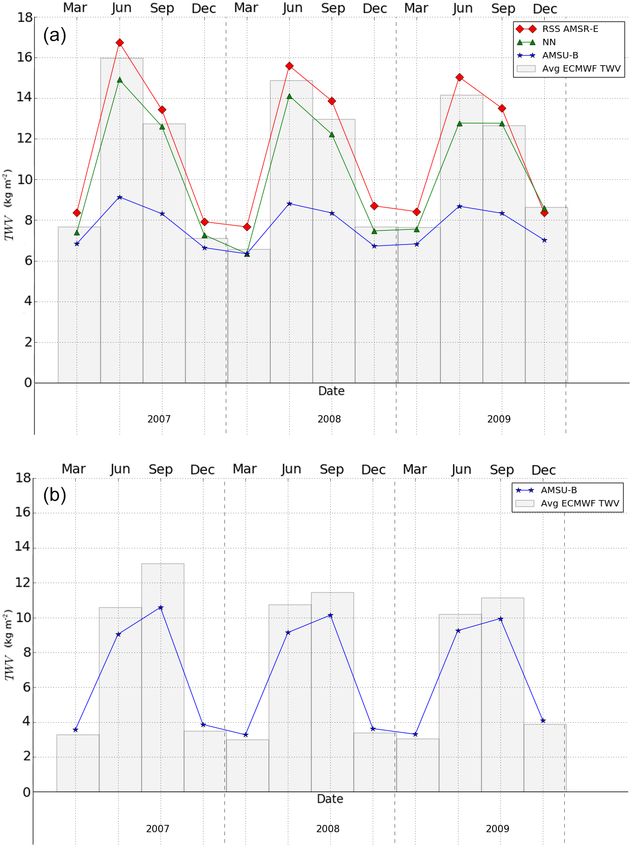
2070                                                        R. C. Scarlat et al.: Retrieval of total water vapour in the Arctic

As shown in Melsheimer and Heygster (2008) – Appendix II,          The final retrieval equation for water vapour content W is
a good approximation for this term is                              then
      Z∞h                                i dT (z)                  W secθ = C0 + C1 log ηc ,                                       (9)
bij ≈    e−τj (z,∞)secθ − e−τi (z,∞)secθ          dz.      (4)
                                            dz                                      B0
                                                                   where C0 = − B      and C1 = B11 characterize the atmospheric
       0                                                                             1
                                                                   attenuation at the channel frequencies used. These calibration
Here, T (z) stands for the temperature profile of the atmo-        parameters are determined from simulated brightness tem-
sphere with height z. To find the relationship between the         peratures based on radiosonde profiles. The simulations were
measured brightness temperature and the water vapour ab-           run using the ARTS (Atmospheric Radiative Transfer Simu-
sorption that does not depend on any other surface parame-         lator) radiative transfer model (Eriksson et al., 2011), which
ter, we require the third brightness temperature measured in       used as input radiosonde data collected from 29 coastal or is-
channel k. With this, a pair of brightness temperature differ-     land WMO (World Meteorological Organization) stations in
ences is available, from which the ratio will be                   the Arctic. The time period for the radiosonde measurements
                                                                   is between 1996 and 2002.
       1Tij − bij    e−2τi secθ − e−2τj secθ                          By replacing the form of ηc from Eq. (7) in the ratio of
ηc ≡                = −2τ secθ               .             (5)
       1Tj k − bj k  e j        − e−2τk secθ                       brightness temperature differences from Eq. (5), we obtain
                                                                   the linear relationship between 1Tij and 1Tj k
   By using the two brightness temperature differences be-
tween three brightness temperatures and taking the ratio of        1Tij () = bij + ηc (W )(1Tj k () − bj k ).                   (10)
these differences, all terms that depend on surface parame-
ters have been simplified and now we have a direct relation-       The brightness temperature differences depend on the sur-
ship between the measured brightness temperatures and at-          face emissivity , while ηc only depends on W . In a 1Tij
mospheric opacity due to water vapour absorption. Following        vs. 1Tj k scatter plot with constant W and for varying ,
the naming convention in Melsheimer and Heygster (2008),           Eq. (10) describes a straight line of slope ηc (W ) that runs
we call the left-hand side of Eq. (5) the ratio of compensated     through the point (bij , bj k ). Because the two bias parameters
brightness temperatures, ηc (containing the correction terms       vary only weakly with W and η, all lines obtained for differ-
bij and bj k ). ηc is independent of any surface contribution,     ent W values will cross or pass very near to one single point
and only influenced by the atmospheric opacity terms τ(i,j,k)      F (Fj k , Fij ), called the focal point (Miao et al., 2001). To find
at the three channel frequencies. These atmospheric opacity        its coordinates, brightness temperature simulations were run
terms in turn are functions of the amount of absorption by         for eleven discrete values of . For the calibration parameters
water vapour and oxygen and can be expressed as                    described above, the simulations are run with the ARTS ra-
                                                                   diative transfer model using Arctic radiosonde profiles with
τi = κvapour,i W + τoxygen,i ,                             (6)     realistic W values as input. For all simulations, the surface
where κvapour,i is the water vapour mass absorption coeffi-        temperature equals the ground-level atmospheric tempera-
cient at channel i, τoxygen,i represents the oxygen contribu-      ture. For each constant W value, a line is fitted to the points in
tion to the atmospheric attenuation at channel i, and W is         the 1Tij vs. 1Tj k scatter plot. The point of least square dis-
the water vapour load. For the band channels around the            tance from all lines will be called the focal point F . By find-
183.31 GHz frequency, the contribution of water vapour to          ing the focal point coordinates we have the relationship be-
the absorption is much stronger than for oxygen, so the            tween the simulated brightness temperature differences and
τoxygen,i term will be neglected henceforth.                       the W values and so are able to fit Eq. (9), which allows us
   The aim is to have a direct connection between the ratio        to determine the constant calibration parameters C0 and C1 .
of brightness temperature and the water vapour content W .         With this method a total of four parameters, two focal point
Using the approximation introduced by Miao (1998), the dif-        coordinates and two atmospheric calibration parameters are
ference of exponentials can be transformed into a product of       derived through the regression fit.
a linear and an exponential function, so eventually we get            The principal problem with the Antarctic algorithm was
                                                                   that the sensitive band channels around the 183.31 GHz fre-
           h                               i
ηc = exp B0 + B1 W secθ + B2 (W secθ )2 .                  (7)     quency will reach saturation with relatively low amounts
                                                                   of atmospheric water vapour (Selbach, 2003). This means
Here B0 , B1 and B2 depend on the mass absorption coeffi-          that after crossing a certain threshold value for W , the
cients k for the three channels and are called bias parame-        brightness temperature Tb does not vary with increasing W .
ters. Compared to the first two terms under the exponent the       Therefore, when one channel reaches saturation, it can no
quadratic term is negligible small, so the logarithm of Eq. (7)    longer be used in the retrieval triplet for higher W val-
becomes                                                            ues. For the first channel triplet (183.31 ± 7, 183.31 ± 3
                                                                   and 183.31 ± 1 GHz), the first channel (AMSU-B channel
log ηc = B0 + B1 W secθ.                                   (8)     18 at 183.31 ± 1 GHz) reaches saturation at 1.5 kg m−2 . To

Atmos. Meas. Tech., 11, 2067–2084, 2018                                               www.atmos-meas-tech.net/11/2067/2018/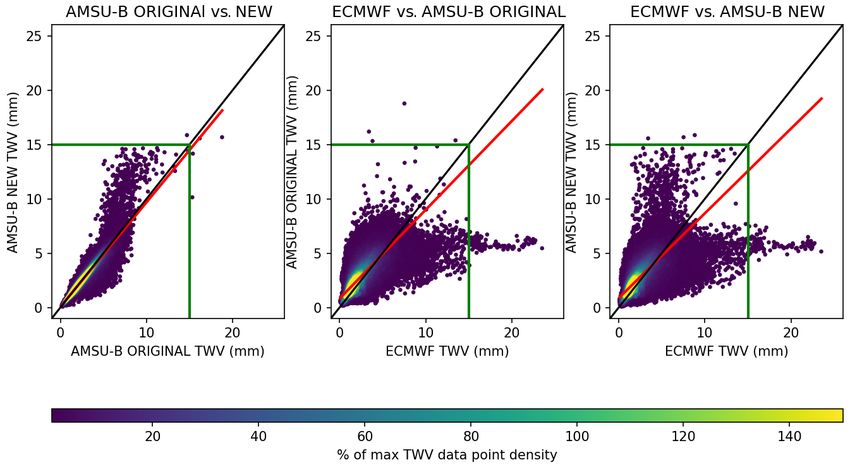
R. C. Scarlat et al.: Retrieval of total water vapour in the Arctic                                                          2071

achieve a practical W retrieval range, the channel triplet (17,   becomes
20, 19, i.e. 150, 183.31 ± 7 and 183.31 ± 3 GHz) is used
for values higher than 1.5 kg m−2 and can function up to          1Tij ≡ Tb,i − Tb,j
7 kg m−2 when channel 19 reaches saturation. As a practi-

                                                                  1Tij = (T0 − Tc ) rj e−2τj secθ − ri e−2τi secθ + bij ,     (12)
cal test for when the algorithm should switch between the
two channel triplets, the saturation point for a given channel
                                                                  where r is the ground reflectivity (1 − ), and bij is the same
k, as defined in Miao et al. (2001), is the W threshold value
                                                                  as in Eq. (4), because it does not depend on the surface emis-
after which Tb,j ≤ Tb,k , or simply
                                                                  sivity . The corresponding compensated ratio of brightness
                                                                  temperature differences is
Tb,j − Tb,k ≥ 0.                                          (11)
                                                                           1Tij − bij     ri e−2τi secθ − rj e−2τj secθ
This test is based on the threshold at which the brightness       ηc =                  =                              .     (13)
                                                                           1Tj k − bj k   rj e−2τj secθ − e−2τk secθ
temperature of a given channel no longer increases with in-
creasing W . This threshold represents the point at which the     After rearranging terms to resemble the original form in
brightness temperature levels off and then starts to decrease     Eq. (5) we get
again with increasing W . This happens as the signal that
                                                                         ri (e−2τi secθ − e−2τj secθ )

reaches the instrument no longer comes from the entire atmo-                                                   ri
                                                                  ηc =                                 −   1 −
spheric column down to the ground but only from the colder,             rj (e−2τj secθ − e−2τk secθ )          rj
upper part of the atmosphere. In the original version of the                    −2τ secθ
                                                                                e j
Arctic algorithm (Melsheimer and Heygster, 2008), in order                                         .                  (14)
                                                                       e −2τ j secθ − e−2τk secθ
to extend the retrieval range, the above condition has been
relaxed. The saturation cut-off temperature, Tbj − Tb,k ≥ 0       After approximating the difference in exponentials as before,
has been modified to F20,19 (Tbj −Tb,k ≥ F20,19 ), with F20,19    the compensated ratio of brightness temperature differences
being a few kelvins. This modification translates to an in-       becomes
crease in the retrieval range by about 1 kg m−2 at the ex-
                                                                        ri    h                               i
pense of increased error as the channel approaches its sat-       ηc = exp B0 + B1 W sec θ + B2 (W secθ )2
uration limit. If the difference 1Tj k − Fj k is smaller than           rj

−10 K, the corresponding error for the second channel triplet                ri
                                                                     − 1−         C(τj , τk ),                             (15)
(17, 20, 19) is below 0.4 kg m−2 for the retrieval range 1.5–                rj
7 kg m−2 . For the first channel triplet (20, 19, 18), which
has the narrow retrieval range of 0–1.5 kg m−2 , the error is     where
below 0.2 kg m−2 . This particular issue of the relaxed con-
                                                                                         e−2τj secθ
ditions will be addressed in the final algorithm (Sect. 2.7).     C(τj , τk ) =
These specific cases in which the Melsheimer and Heygster                         e−2τj secθ − e−2τk secθ
(2008) algorithm only retrieves data under the relaxed con-       is a slowly varying function that depends only on the atmo-
dition scenario were found to be mostly open-water regions        spheric absorption factors. In order to obtain a simple linear
where the equal emissivity assumption failed. The new com-        relationship between the compensated brightness tempera-
ponents that deal exclusively with retrieval over open water      ture difference and water vapour load W , we rearrange the
use the condition in Eq. (11).                                    above equation into

2.3   Extending the TWV retrieval range                           log ηc 0 = B0 + B1 W secθ + B2 (W secθ )2 .                 (16)

Normally, for TWV values above 7 kg m−2 , saturation occurs       The modified ratio ηc 0 includes the terms depending on the
at channel 19 (183.3 ± 3 GHz). To extend the retrieval range      reflectivities and the C(τj , τk ) function
above this threshold, it is necessary for a new channel to take            ri
its place in the triplet, which means that a new set of assump-   ηc 0 =       ηc + C(τj , τk ) − C(τj , τk ).                (17)
                                                                           rj
tions has to be made about the surface emissivity influence.
Now, the three channels i, j, k represent AMSU-B channels         The final retrieval equation for W is obtained after eliminat-
16, 17 and 20 (89, 150 and 183.31 ± 7 GHz). Because chan-         ing the negligible quadratic term
nel 16 is so far from the other two, we can no longer assume
that it has the same surface emissivity as the others. There-     W secθ = C0 + C1 log ηc 0.                                  (18)
fore, we will have i 6 = j for the new channel i and j = k
is the approximation used as before.                              The difference between ηc 0 and ηc is that the former depends
   If we consider that we have two channels with different        on the surface emissivity through the reflectivities ratio rrji ,
surface emissivities, the brightness temperature difference       while the latter is surface independent. To enable retrieval

www.atmos-meas-tech.net/11/2067/2018/                                                  Atmos. Meas. Tech., 11, 2067–2084, 2018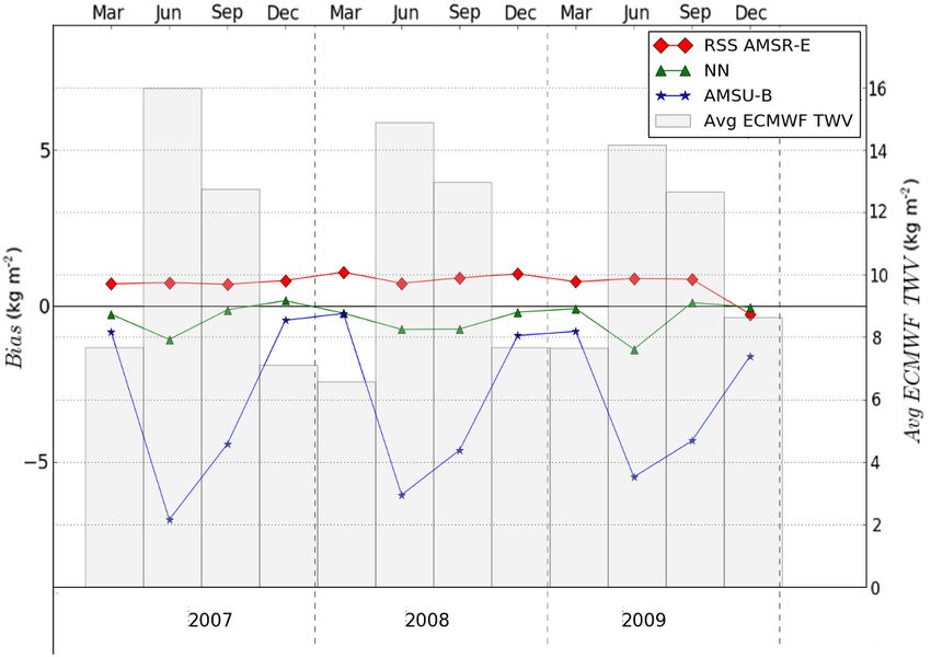
2072                                                          R. C. Scarlat et al.: Retrieval of total water vapour in the Arctic

using Eq. (18), more information is needed about the be-             It is indicated by Melsheimer and Heygster (2008) that this
haviour of the surface emissivities at 150 and 89 GHz. Di-           is just partial compensation for the contribution of surface
rect information about the surface emissivity for every satel-       emissivity. The SEPOR-POLEX measurements were made
lite footprint is not available so we need to parameterize the       in the winter season and therefore do not take into account
emissivity and obtain a constant reflectivity ratio that would       the melt processes that take place in summer, which can sig-
only roughly depend on the surface type (ocean/ice/land).            nificantly alter the emissivity behaviour of the surface (Ton-
Identifying the major surface types in the Arctic is another         boe et al., 2003). Because other resources on the subject are
task that has to be integrated into the algorithm. Because           sparse this was the only way to include the effects of surface
at the time no ocean surface emissivity information was              emissivity in TWV retrievals.
readily available and a proof of concept was first needed               Besides the two parameters C0 and C1 , which account
over regions with low enough TWV, the Melsheimer and                 for the atmospheric conditions in the Arctic, the modified
Heygster (2008) algorithm extension was adapted only for             ratio of compensated brightness temperatures ηc 0 requires
sea-ice surfaces. The sea-ice surface emissivity data were           the C(τj , τk ) term that depends on the atmospheric opaci-
obtained from the Surface Emissivities in Polar Regions-             ties and thus, directly on TWV. If one studies the behaviour
Polar Experiment (SEPOR-POLEX measurement campaign                   of C(τj , τk ) with increasing TWV for values above 7 kg m−2
in 2001). This campaign used an aircraft-mounted instru-             the function varies only a little, and it can be approximated by
ment, the Microwave Airborne Radiometer Scanning System              a constant. According to Melsheimer and Heygster (2008),
(MARSS), which possesses two microwave channels of fre-              a variation in C(τj , τk ) between 1.0 and 1.2 will result in
quencies similar to those required for the algorithm exten-          a change in C0 and C1 in the third significant digit. In to-
sion. For AMSU-B channel 16 at 89 GHz, there exists the              tal we have the two focal point coordinates, the atmospheric
MARSS channel 88.992 GHz, and for AMSU-B channel 20                  parameters C0 and C1 , and the slowly varying function ap-
at 150 GHz there exists a corresponding MARSS channel at             proximated by the constant C(τj , τk ) ≈ 1.1. The set of four
157.075 GHz. This difference of 7 GHz does not pose sig-             parameters is determined through regression by using simu-
nificant issues for the retrieval using the 150 GHz channel.         lated brightness temperatures and atmospheric data from ra-
The difference between measurements at 150 and 157 GHz               diosonde profiles as described in Sect. 2.2.
is between ±0.01 calculated from the in situ measurements               The weakness of the extended algorithm is its sensitivity
(Selbach et al., 2003; Selbach, 2003), while the emissivity          to changes in the reflectivity ratio. In other words, for sea-ice
variability for the different ice types is greater than this dif-    surfaces where the surface emissivity deviates within the un-
ference. Because of this, the impact on the final retrieval is       certainty limits of σrj /ri = 0.09 (Melsheimer and Heygster,
considered negligible.                                               2008) from the constant emissivities ratio used, the retrieval
   To obtain the reflectivity ratio, the regression of 89 as a      error can be as high as 3 kg m−2 .
function of 150 was calculated:                                        Because of the specific channel triplet used by each sub-
                                                                     algorithm, the set of four calibration parameters has to be
89 = a + b150 .                                           (19)     determined for the low TWV, mid-TWV and extended-TWV
                                                                     cases. In the new algorithm, two extra sets of calibration pa-
For the ratio of reflectivities to be constant it has to be in-      rameters are required for the mid-TWV over open water and
dependent of the variable emissivities. Because of this the          extended TWV over open-water components.
regression was constrained, so 89 (150 = 1) ≈ 1. The physi-
cal meaning of this is that the emissivity for the two channels
cannot be greater than 1. Using the constraint above means           2.4   Modifying the extended algorithm for use over
that a + b ≈ 1, and so the reflectivity ratio only depends on              open ocean
the regression relationship coefficient b
r150  1                                                              In Melsheimer and Heygster (2008) the possibility of using
     ≈ .                                                    (20)     the same technique of incorporating surface emissivity infor-
r89   b
                                                                     mation for the purpose of using the extended-range compo-
   From the data points over sea ice, the following regression       nent over open-water regions in addition to sea-ice-covered
relationship was found by Melsheimer and Heygster (2008)             areas was considered a possible improvement but was not in-
for emissivity at 89 and 150 GHz:                                    vestigated further.
                                                                        In order to determine the feasibility of this option, a suit-
89 = 0.1809 + 0.8192 · 150 .                              (21)     able linear relationship between surface emissivities at chan-
                                                                     nels 150 and 89 GHz is required. By reusing the retrieval
By replacing the coefficient b in Eq. (20) we have the reflec-       equation and replacing the calibration coefficients and the ra-
tivity ratio                                                         tio of reflectivities, a separate module can be implemented to
r150                                                                 retrieve water vapour in the extended range only over open
     = 1.22.                                                (22)     water.
r89

Atmos. Meas. Tech., 11, 2067–2084, 2018                                                www.atmos-meas-tech.net/11/2067/2018/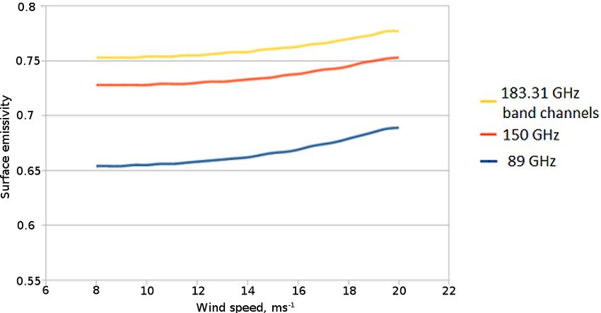
R. C. Scarlat et al.: Retrieval of total water vapour in the Arctic                                                           2073

Figure 1. Ocean surface emissivities’ dependence on wind speed.

   The ocean emissivity model FASTEM (FAST surface
Emissivity Model for microwave frequencies) takes into ac-
count the characteristics of the AMSU-B instrument, sea sur-
face temperature and roughness (Hocking et al., 2011). The
parameter that was found to determine strong variation in
surface emissivity is the ocean surface roughness. Surface
roughness in turn is determined by wind speeds. At the typ-
ical range of values encountered in the Arctic (8–20 m s−1 ),
surface emissivity is determined mainly by wind speed. Fig-
ure 1 shows the behaviour of the ocean surface emissivi-            Figure 2. Regression plot for ocean surface emissivity at 89 and
                                                                    150 GHz (a) and at 150 and 183 GHz (b).
ties for the five channel frequencies of the AMSU-B instru-
ment. Because the frequencies of the three band channels
around 183.3 GHz are so close to each other, the correspond-
                                                                    reflectivities:
ing emissivities are almost identical and thus represented by
only one curve on the graph. It is important to notice the large    r150
                                                                         = 0.7875.
difference between the curve for 89 and the one for 150 GHz,        r89
which illustrates why the assumption of equal emissivities
cannot be sustained for these pairs of channels. Also, the dif-
                                                                      Using this relationship, the calibration parameters C0 and
ference between the 183.3 GHz and the 150 GHz curves must
                                                                    C1 were also determined from a regression between W from
be noted, because it is neglected when using the assumption
                                                                    radiosonde profiles and simulated brightness temperatures as
of equal surface emissivity for the medium TWV retrieval
                                                                    described in Sect. 2.2.
range.
                                                                    2.6   Ocean surface emissivity for the mid-range 150,
2.5   Ocean surface emissivity for the extended range 89,
                                                                          183.3 ± 7 and 183.3 ± 3 GHz triplet set-up
      150, 183.3 ± 7 GHz triplet set-up
                                                                    One of the error sources in the original algorithm was the
Following the same method as for the extension over sea ice,        assumption of equal surface emissivity for the 150 and
through a linear regression between the ocean surface emis-         the 183.3 GHz band channels. Over open-ocean, the differ-
sivity at 150 and at 89 GHz (panel a of Fig. 2), we found the       ences in surface emissivity at these frequencies can lead to
following linear relationship in the form of Eq. (10).              a positive bias in the TWV retrieval. Following the same
                                                                    methodology as for the lowermost channel triplet (89, 150,
                                                                    183.3 ± 7 GHz), a linear relationship can be retrieved from
89 = 1.2698 · 150 − 0.2687.                               (19)    simulated ocean surface emissivity data for the frequency
                                                                    triplet (150, 183.3 ± 3, 183.3 ± 7 GHz). From this, a reflec-
   For the emissivity of sea ice, studied for the first retrieval   tivity ratio can be obtained and used in a modified retrieval
range extension, the constraint 89 (150 = 1) ≈ 1 had to be        equation. This modification leads to an improvement in the
imposed on the system in order to express the ratio of re-          bias when retrieving in the TWV range 2–6 kg m−2 over ice-
flectivities as a constant of the form shown in Eq. (7), inde-      free ocean surfaces.
pendent of variable surface emissivity. Following the same             Following the regression fit in Fig. 2b we obtained the
logic, from the linear expression above we obtain the ratio of      linear relationship for ocean surface emissivity at 150 and

www.atmos-meas-tech.net/11/2067/2018/                                                 Atmos. Meas. Tech., 11, 2067–2084, 2018
2074 R. C. Scarlat et al.: Retrieval of total water vapour in the Arctic
Figure 3. C(τj , τk ) parameter for the mid-TWV algorithm (a) and for extended-TWV algorithm (b). The dashed horizontal lines represent
the variability interval for the C(τj , τk ) parameter inside the TWV range corresponding to each case.
183 GHz, retrieval over open-water areas. This allows for retrieval over
a greater spatial domain, as the original algorithm could only
150 = 1.1022 · 183 − 0.1028, (23)
use the mid-TWV sub-algorithm over open water for TWV
from which we obtain the ratio of reflectivities, values up to 7 kg m−2 .
r183 Another addition to the original AMSU-B algorithm is
= 0.9073. (24) that the mid-TWV sub-algorithm differentiates between sea
r150
ice/land and open water and has different retrieval equations
In addition to the C0 and C1 parameters, the C(τj , τk ) for each of the two cases. We believe that this is a more physi-
function that depends on atmospheric opacity is necessary cally consistent treatment than using the equal emissivity as-
for retrieval when a different surface emissivity is consid- sumption. The specific open-water module uses the regres-
ered (Sect. 2.3). This function depends directly on TWV and sion relationship in Eq. (23), while the sea-ice/land module
it has been shown that above 7 kg m−2 it is constant for the uses the equal emissivity assumption. In the original algo-
89 and 150 GHz frequencies. rithm, mid-TWV retrieval over open water also operates un-
For the channels used in the mid-TWV range retrieval der the equal emissivity assumption.
module, the function C(τj , τk ) behaves differently than for The algorithm for low-TWV uses AMSU-B channels 20,
the extended-TWV channels. Between 2 and 6 kg m−2 it 19 and 18 for the retrieval range 0 to 1.5 kg m−2 . These are
drops rapidly from 1.4 down to 1.0 (Fig. 3), but it has been the band channels around the strong water vapour line at
found (Melsheimer and Heygster, 2008) that changes of the 183.31 GHz, and have the best accuracy and present the low-
order of 0.2 in C(τj , τk ) lead to differences in the third signif- est error as the assumption of equal surface emissivity is valid
icant digit of the C0 and C1 parameters, which is small com- for these three frequencies.
pared to other error contributions. In the process of modify- The mid-TWV algorithm using AMSU-B channels 17, 20
ing the mid-TWV algorithm, the C(τj , τk ) was recalculated and 19 takes over retrieval up to 7 kg m−2 . It is assumed
for the 183±7 and the 150 GHz channels and set as a con- to be independent of the surface type but the retrieval error
stant, C(τj , τk ) ≈ 1.15, in the retrieval Eq. (18). might increase when approaching the upper retrieval limit.
The assumption of equal emissivity is still used over sea-
2.7 TWV algorithm synthesis
ice-covered surfaces, even though there are some differences
The final structure of the new algorithm comprises a collec- because of the introduction of the 150 GHz channel instead
tion of independent retrieval modules, each tuned to a differ- of the 183 ± 1 GHz channel. Because of this difference in
ent set of surface and atmospheric parameters. This structure real surface emissivity a positive bias of up to 0.5 kg m−2 is
can be viewed in Table 1 where the SSM/T2 Antarctic algo- possible (Selbach, 2003). Over areas with sea-ice concentra-
rithm by Miao et al. (2001), the original AMSU-B Arctic re- tion below 80 %, the specific open-water sub-module of the
trieval algorithm by Melsheimer and Heygster (2008) and the mid-TWV algorithm uses the ratio of reflectivities at 183 and
new AMSU-B algorithm are described. The main modules 150 GHz in order to account for the different surface emissiv-
represent the three different channel triplets, low, middle and ities of open water at these frequencies.
high, that are used in the different retrieval ranges of TWV. The extended-TWV module uses the channels 20, 17 and
Further differentiation into sub-modules is made by distin- 16 to retrieve TWV in the range 7–15 kg m−2 . Previously, the
guishing between sea ice or open water, leading to five mod- retrieval from these channels was restricted to sea-ice regions
ules in total. One of the main differences between the new and because of the simplified treatment of the surface emis-
and the original AMSU-B algorithm is the use of the emissiv- sivity difference, the error can reach 3 kg m−2 . Similarly with
ity relationship in Eq. (19) for applying the extended-TWV the mid-TWV module above, a dedicated open-water version
Atmos. Meas. Tech., 11, 2067–2084, 2018 www.atmos-meas-tech.net/11/2067/2018/R. C. Scarlat et al.: Retrieval of total water vapour in the Arctic 2075
Table 1. Comparative structure of three TWV retrieval algorithms. SI represents sea ice only and OW – open water as surface types where
the individual modules can be applied. L, M and E represent low-, mid- and extended-range TWV retrieval modules.
Method Sub-modules Channel frequency (GHz) Channel no. TWV (kg m−2 ) Surface
L-TWV 183.31 ± 1, ±3, ±7 2, 3, 4∗ 0–1.5 All
Miao algorithm M-TWV 183.31 ± 3, ±7, 150 3, 4, 5∗ 1.5–6 All
L-TWV 183.31 ± 1, ±3, ±7 18, 19, 20 0–1.5 All
Original AMSU-B M-TWV 183.31 ± 3, ±7, 150 19, 20, 17 1.5–7 All
E-TWV – SI 183.31 ± 7, 150, 89 20, 17, 16 7–15 SI
L-TWV 183.31 ± 1, ±3, ±7 18, 19, 20 0–1.5 All
M-TWV 183.31 ± 3, ±7, 150 19, 20, 17 1.5–7 SI/land
New AMSU-B M-TWV – OW 183.31 ± 3, ±7, 150 19, 20, 17 1.5–7 OW
E-TWV – SI 183.31 ± 7, 150, 89 20, 17, 16 7–15 SI
E-TWV – OW 183.31 ± 7, 150, 89 20, 17, 16 7–15 OW
∗ The Miao algorithm was developed for the SSM/T2 instrument and for the Antarctic region.
of the extended-TWV module uses the ratio of reflectivities By mapping (not shown) the pixels according to the con-
at 89 and 150 GHz over scenes with mixed water and sea ice. ditions used in their retrieval with the original algorithm, we
The set of four calibration parameters has to be determined found that the values near the saturation limit retrieved un-
for each of the low TWV, mid-TWV and extended TWV as der the relaxed conditions in most cases account for open-
each of these sub-modules uses a different channel triplet. water or mixed-water/sea-ice surfaces. This is where the
Two extra sets are determined for the new open-water mid- equal emissivity assumption breaks down because the mi-
and extended-TWV retrieval sub-modules because they use crowave emissivity of water is much lower than that of sea
modified retrieval equations. ice producing an increased retrieval error. In this new algo-
rithm we propose using a specific method for those areas.
2.8 How the retrieval works For the mid- and extended-range TWV algorithms there is
a further differentiation in the modules used between sea-ice
One of the critical points in all of the AMSU-B algorithms and open-water surfaces. Based on our experience, a thresh-
is to correctly identify when a particular triplet of chan- old of 80 % sea-ice concentration was chosen in order to dif-
nels becomes saturated in order to switch to the next avail- ferentiate the typically dry areas of high sea-ice concentra-
able triplet. In the initial Antarctic algorithm paper by (Miao tion in the central Arctic from the regions with a larger ra-
et al., 2001), this was accomplished by checking the sign of tio of open water to sea ice, where higher atmospheric wa-
the brightness temperature difference using the condition in ter vapour loads are expected. In these peripheral regions the
Eq. (11). new algorithm is employed. In all areas with sea-ice concen-
In order to extend the coverage while keeping the retrieval tration above 80 % the retrieval technique from Melsheimer
error reasonably low, the constraint above was relaxed in and Heygster (2008) is used, which is better suited for the
(Melsheimer and Heygster, 2008) by allowing the brightness very low atmospheric water vapour values encountered in
temperature difference to go slightly above zero so that, in this region.
the end, the following condition is applied: To illustrate how the new algorithm works with these new
sets of conditions we will present each step with its differ-
ences to the previous method.
Tb,j − Tb,i < Fi,j . (25)
1. The algorithm begins by using the full set of five bright-
Fi,j is the focal point calculated for a particular channel ness temperatures of the AMSU-B instrument. In the
triplet. It usually has a value of a few kelvins. The retrieval previous method, it would first identify pixels where the
will work as long as the sign of the brightness temperature conditions
differences ratio ηc is positive. L L
This relaxed condition allows the channel triplet to be used Tb,19 − Tb,18 < F19,18 and Tb,20 − Tb,19 < F20,19
until its high-absorption channel approaches saturation and
allows an extension of the retrieval range of that triplet by L
hold true. Here F19,18 L
and F20,19 are the pairwise focal
up to 1 kg m−2 . The disadvantage of this relaxed condition is points for channel pairs (18, 19) and (19, 20). When this
that the retrieval error also increases when a channel in the condition is fulfilled it allows for the channel triplet (18,
triplet is close to saturation. 19, 20) to be used for the range up to 2 kg m−2 . Because
www.atmos-meas-tech.net/11/2067/2018/ Atmos. Meas. Tech., 11, 2067–2084, 20182076 R. C. Scarlat et al.: Retrieval of total water vapour in the Arctic
the retrieval range of the first two channel triplets (low 2.9 Comparing the new retrieval with other TWV
and middle ranges) overlaps around 2 kg m−2 we will retrieval products
keep the stricter condition from the Antarctic algorithm
(Miao et al., 2001). For a comparison we use daily averages for 30 consecutive
days in each of 4 months, September, March, June and De-
Tb,19 − Tb,18 < 0, Tb,20 − Tb,19 < 0
cember, which represent the variability of the atmospheric
For these pixels the low-TWV algorithm is applied. parameters and sea-ice extent. September and March repre-
sent the two extremes of sea-ice extent. The minimum extent
2. If the first condition fails, the second one is checked. In in September is usually coupled to warmer air and higher
the previous method this was atmospheric water vapour loads. The maximum extent in
M
Tb,20 − Tb,19 < F20,19 M
and Tb,17 − Tb,20 < F17,20 . March corresponds to lower air temperatures and a drier at-
mosphere. June and December represent transition periods
Continuing from the strict zero-threshold condition for between the two extremes.
the low TWV, the new condition threshold is In order to obtain a bigger data sample we ran this analysis
using daily averaged data for 3 consecutive years from 2007
2 (a)
to 2009. The geographical domain we chose represents the
Tb,19 − Tb,18 ≥ 0 and Tb,20 − Tb,19 < 0 entire Northern Hemisphere above 50◦ N latitude. Though
and Tb,17 − Tb,20 < 0. the very first retrieval was targeted towards the central Arc-
tic region, this was because the atmospheric water vapour
This test is performed for pixels with over 80 % sea-ice load over this region was low enough for a retrieval. After the
concentration. Where this is true, the original mid-TWV subsequent extensions of the retrievable TWV range, the ge-
retrieval is used. ographical domain for applying the algorithm has increased
as well. For the purpose of this work we have arbitrarily cho-
2 (b)
sen this 50◦ N limit because that is the approximate latitude
Over open water and scenes with ice concentration be-
at which the water vapour load in winter is low enough to al-
low 80 % in the middle TWV range, the algorithm now
low a time-consistent retrieval with the newest version of the
uses a somewhat different condition
algorithm. All land masses in this region are also included
X because the method is able to retrieve TWV there if the val-
Tb,19 − Tb,18 ≥ 0 and Tb,20 − Tb,19 < F20,19
X ues are low enough. For example, Greenland is always in-
and Tb,17 − Tb,20 < F17,20
cluded in the retrieval because the atmosphere above it is dry
Condition 2(b) means that the pixels which were pre- throughout the year.
viously retrieved under the equal emissivity assumption From AMSU-B data we produce two versions of the TWV
over open water will now be treated separately accord- product, one retrieved with the original Melsheimer and
ing to their surface type, taking into account the surface Heygster (2008) method and the other with the new algo-
emissivity component. Those pixels that are at the satu- rithm. The calibration parameters we derived separately for
ration limit for the middle range but do not contain open each channel combination with the corresponding linear re-
water are being flagged for further processing with the lationships between surface emissivities from the same batch
extended-range sea-ice algorithm. This would include of radiosonde TWV data.
pixels retrieved above land in less dry conditions (in the First we want to see how the new retrieval method per-
Arctic case this means TWV > 2 kg m−2 ). forms against the original one and hence test both methods
against two other TWV products chosen as benchmarks in
3. When applying the extended-TWV algorithm, the re- this field. The first benchmark is the ECMWF (European
maining pixels are tested for Centre for Medium-Range Weather Forecasts) ERA-Interim
X
Tb,17 − Tb,20 < F17,20 X
and Tb,16 − Tb,17 < F16,17 , (Dee et al., 2011) reanalysis model data from which TWV
values were derived.
and if true are processed. In addition to this test for The second data set is the TWV product from Remote
channel saturation, the data are again classified for their Sensing Systems (RSS), which uses AMSR-E brightness
surface type, and only sea-ice or open-ocean areas are temperatures and an algorithm adapted from Wentz (1997).
kept, excluding land. This surface classification is done This retrieval algorithm has been developed for global cov-
for all channels by a comparison with sea-ice concentra- erage and works over all ice-free ocean surfaces. Because of
tion maps derived using the ARTIST Sea Ice concentra- this it can cover a large range of TWV values (0–75 kg m−2 ),
tion retrieval (Spreen et al., 2008) from SSMIS (Special but it was not specifically tuned for the dry Arctic conditions.
Sensor Microwave Imager/Sounder) or AMSR-E (Ad- This data set covers the entire 9-year lifespan of AMSR-E,
vanced Microwave Scanning Radiometer – Earth Ob- has been used for creating derived products (Smith et al.,
serving System) data depending on the retrieval date. 2013), is validated against ship-based observations (Szczo-
Atmos. Meas. Tech., 11, 2067–2084, 2018 www.atmos-meas-tech.net/11/2067/2018/R. C. Scarlat et al.: Retrieval of total water vapour in the Arctic 2077
drak et al., 2006) and hence is considered a good benchmark from 2007 to 2009 in order to see how the total area of re-
against which the new AMSU-B retrieval can be compared. trievable pixels is affected by the new method (Fig. 6). In
A third test data set was obtained from the Bobylev et al. the colder months of March and December the benefit of
(2010) algorithm. This method is a neural-network-based ap- the new method is marginal because of the larger sea-ice ex-
proach designed specifically for the ice-free regions in the tent (when compared to the summer months) and the overall
Arctic. As a training data set for the neural network the au- low water vapour burden of the atmosphere. In these months
thors used radiosonde data from Russian polar stations. The we can observe small increases of 17.4 and 21.18 % respec-
method is able to retrieve low TWV values over open-ocean tively, compared to the coverage of the original algorithm.
areas using the same AMSR-E instrument as the RSS TWV For September and June the number of retrievable pixels in-
product with similar TWV value ranges. This neural network crease by 152 and 176 % (Fig. 6). This change is significant
approach is proven to have a smaller root mean square er- considering that these areas were beyond the retrieval capa-
ror than the Wentz global algorithm used in the RSS TWV bilities of the original method.
product. These three retrievals are compared over one com- ECMWF ERA-Interim reanalysis data were used as refer-
mon valid spatial domain (only open water) while using the ence in order to compare the original method and the new
ECMWF TWV data as reference. one. The ECMWF TWV information was directly compared
to collocated daily averages from both algorithms. In terms
of correlation with the ECMWF, the two algorithms vary sig-
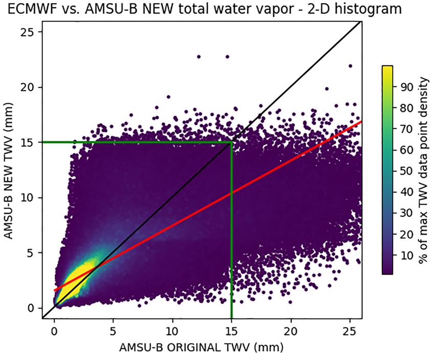
3 Results and discussion nificantly (Fig. 7).
The new method matches the correlation of the original
3.1 Comparison of results to Melsheimer and one for the month of March (0.86), and even surpasses it for
Heygster (2008) December (0.82 vs. 0.77). In the months with moist condi-
tions and lower sea-ice extent, June and September, the cor-
Independent of the comparison benchmark, an important dif- relation drops to 0.36 and 0.32 vs. 0.57 and 0.61. Comparing
ference between the original and the new retrieval is the area this with the results in Fig. 6 shows that in the months where
the algorithm can cover to retrieve TWV in the Arctic. Be- the spatial contribution of the improved algorithm is greater,
cause both algorithms use the same instrumental input, a one- the correlation drop is more significant. For a more de-
to-one comparison of coverage represented as the number of tailed look into the differences between the original and new
valid retrievable pixels is possible. AMSU-B methods, a side-by-side comparison is presented
Figure 4 shows two examples in the coverage difference in Fig. 8. Here the original and new algorithm are compared
between the original and the new retrieval, for one summer with each other and then individually with ECMWF TWV
and one winter day. The greatest benefit of the new retrieval over the same common domain valid for both retrievals. One
is that large areas in the North Atlantic and Pacific oceans major difference between the two algorithms is in the way the
can now be covered. The only limitation of the method is the mid-TWV retrieval is performed. The new algorithm uses a
amount of water vapour present in the atmosphere and, for dedicated open-water sub-module, while the original algo-
the extended-range module, the presence of either an open- rithm treats all surface types the same in this retrieval range.
water or sea-ice-covered surface. In both the summer and While the small differences in calibration parameters can
winter cases the new method has a larger coverage area, with cause minor differences in the low-TWV domain, where the
the biggest difference being seen in the summer case. To add retrieval equations are identical, the different treatment of the
to this analysis, Fig. 5 presents the frequency of retrieval for surface type causes a larger deviation between the results
the new and the original retrieval versions when looking at at the upper limit of the mid-TWV range. Another modi-
the months of June and December for the whole 3-year inter- fication that has an impact on the new retrieval is the dif-
val studied. Each pixel value represents the number of times ferences in trigger thresholds, which cause the algorithm to
that particular region has been present in the daily retrieval switch to a different retrieval module. These thresholds and
maps for the test time series. The minimum value shown is the differences between the new and original versions have
five, while the maximum is 90 days. As in the 1-day example been described in Sect. 2.8. Because of the stricter switching
of Fig. 4, the increase in coverage for the month of June is ev- condition, the new algorithm switches to the extended-range
ident, with the addition of North Atlantic and Pacific Ocean retrieval module earlier than the original algorithm and re-
regions where the water vapour values are within the retrieval trieves higher TWV values. These data points, which are re-
range. For December the frequency of retrieval has improved trieved with the extended-range module in the new version
since these same ocean regions can now be retrieved more and with the mid-TWV module in the original one, can be
consistently with the new algorithm. seen as a higher AMSU-B new TWV values which deviate
When comparing the two AMSU-B retrieval methods for from the identity line in the left panel of Fig. 8. The compar-
the whole testing time series we look at monthly averages ison of the new algorithm with ECMWF TWV in the right-
compiled from swath data for each method. The compari- most panel of the same figure indeed shows a similar cloud
son was done for the representative 4 months of each year
www.atmos-meas-tech.net/11/2067/2018/ Atmos. Meas. Tech., 11, 2067–2084, 20182078 R. C. Scarlat et al.: Retrieval of total water vapour in the Arctic Figure 4. Daily TWV maps of the Northern Hemisphere obtained from the new algorithm (a, c) and compared to the original AMSU-B algorithm (b, d). The days represented here are 1 June 2009 for (a) and (b), and 1 December 2009 for (c) and (d). of overestimated data points closer to the maximum retrieval tently cover regions where a complete data gap existed in limit of the algorithm. mixed-sea-ice/open-water regions. In these areas other re- In Fig. 9, where the new algorithm is compared against trieval methods, like the AMSR-E-based ones presented in ECMWF TWV over its full spatial domain of valid retrievals, Sect. 2.8, cannot function because of the presence of sea ice, a higher uncertainty of data points with larger TWV values while the original AMSU-B algorithm could not retrieve any- is evident. The scatter in the retrieved data increases with the thing because of the presence of open water and high TWV retrieved TWV value. When the retrieved values approach values. 15 kg m−2 the involved channels are near the saturation limit, When considering the difference between the ECMWF so the true value may well exceed this retrieval limit. As data and the AMSU-B retrieval, the highest bias is again a practice for future studies we recommend only using re- seen in the warmer months (Fig. 10). Following the corre- trieval values up to 14 kg m−2 . It is, however, important to lation results shown in Fig. 7, the higher variability of the note that the majority of data points retrieved fall within new AMSU-B retrieval is confirmed by the root mean square the 0–6 kg m−2 interval, which matches well with the model difference against ECMWF data, which are represented by data. The extended-range retrieval represents the maximum the error bars in Fig. 10. coverage that can be obtained with this instrument and al- The bias behaviour versus ECMWF has changed from the gorithm combination. This increased coverage with the price original to the new algorithm. Both retrievals follow the same of increased uncertainty represents the only way to consis- pattern of low bias in winter and higher bias in the sum- Atmos. Meas. Tech., 11, 2067–2084, 2018 www.atmos-meas-tech.net/11/2067/2018/
You can also read