Inter-Comparison of the Spatial Distribution of Methane in the Water Column From Seafloor Emissions at Two Sites in the Western Black Sea Using a ...
←
→
Page content transcription
If your browser does not render page correctly, please read the page content below
ORIGINAL RESEARCH
                                                                                                                                           published: 28 July 2021
                                                                                                                                   doi: 10.3389/feart.2021.626372

                                            Inter-Comparison of the Spatial
                                            Distribution of Methane in the Water
                                            Column From Seafloor Emissions at
                                            Two Sites in the Western Black Sea
                                            Using a Multi-Technique Approach
                                            Roberto Grilli 1*, Dominique Birot 2, Mia Schumacher 3, Jean-Daniel Paris 4, Camille Blouzon 1,
                                            Jean Pierre Donval 2, Vivien Guyader 2, Helene Leau 2, Thomas Giunta 2, Marc Delmotte 4,
                                            Vlad Radulescu 5, Sorin Balan 5,6, Jens Greinert 3 and Livio Ruffine 2
                                            1
                                              CNRS, Univ Grenoble Alpes, IRD, Grenoble INP, Grenoble, France, 2Département Ressources Physiques et Ecosystèmes de
                                            Fond de Mer (REM), IFREMER, Plouzané, France, 3GEOMAR Helmholtz Centre for Ocean Research, Kiel, Germany, 4Laboratoire
                                            des Sciences du Climat et de l’Environnement, LSCE/IPSL, CEA-CNRS-UVSQ, Gif-sur-Yvette, France, 5National Institute of
                                            Marine Geology and Geoecology–GeoEcoMar, Bucharest, Romania, 6Faculty of Geology and Geophysics, Doctoral School of
                                            Geology, University of Bucharest, Bucharest, Romania

                             Edited by:
                     Martin Scherwath,
                                            Understanding the dynamics and fate of methane (CH4) release from oceanic seepages on
         University of Victoria, Canada
                                            margins and shelves into the water column, and quantifying the budget of its total
                        Reviewed by:
                            Xiaole Sun,     discharge at different spatial and temporal scales, currently represents a major
        Baltic Sea Centre, Stockholm        scientific undertaking. Previous works on the fate of methane escaping from the
                    University, Sweden
                        Thomas Pape,
                                            seafloor underlined the challenge in both, estimating its concentration distribution and
       University of Bremen, Germany        identifying gradients. In April 2019, the Envri Methane Cruise has been conducted onboard
                   *Correspondence:         the R/V Mare Nigrum in the Western Black Sea to investigate two shallow methane seep
                          Roberto Grilli
                                            sites at ∼120 m and ∼55 m water depth. Dissolved CH4 measurements were conducted
                   roberto.grilli@cnrs.fr
                                            with two continuous in-situ sensors: a membrane inlet laser spectrometer (MILS) and a
                    Specialty section:      commercial methane sensor (METS) from Franatech GmbH. Additionally, discrete water
         This article was submitted to      samples were collected from CTD-Rosette deployment and standard laboratory methane
                        Biogeoscience,
               a section of the journal
                                            analysis was performed by gas chromatography coupled with either purge-and-trap or
            Frontiers in Earth Science      headspace techniques. The resulting vertical profiles (from both in situ and discrete water
       Received: 05 November 2020           sample measurements) of dissolved methane concentration follow an expected
            Accepted: 06 July 2021
                                            exponential dissolution function at both sites. At the deeper site, high dissolved
           Published: 28 July 2021
                                            methane concentrations are detected up to ∼45 m from the seabed, while at the sea
                                Citation:
      Grilli R, Birot D, Schumacher M,      surface dissolved methane was in equilibrium with the atmospheric concentration. At the
     Paris J-D, Blouzon C, Donval JP,       shallower site, sea surface CH4 concentrations were four times higher than the expected
        Guyader V, Leau H, Giunta T,
   Delmotte M, Radulescu V, Balan S,
                                            equilibrium value. Our results seem to support that methane may be transferred from the
 Greinert J and Ruffine L (2021) Inter-      sea to the atmosphere, depending on local water depths. In accordance with previous
Comparison of the Spatial Distribution
                                            studies, the shallower the water, the more likely is a sea-to-atmosphere transport of
of Methane in the Water Column From
Seafloor Emissions at Two Sites in the       methane. High spatial resolution surface data also support this hypothesis. Well localized
    Western Black Sea Using a Multi-        methane enriched waters were found near the surface at both sites, but their locations
                   Technique Approach.
             Front. Earth Sci. 9:626372.
                                            appear to be decoupled with the ones of the seafloor seepages. This highlights the need of
      doi: 10.3389/feart.2021.626372        better understanding the processes responsible for the transport and transformation of the

Frontiers in Earth Science | www.frontiersin.org                                 1                                            July 2021 | Volume 9 | Article 626372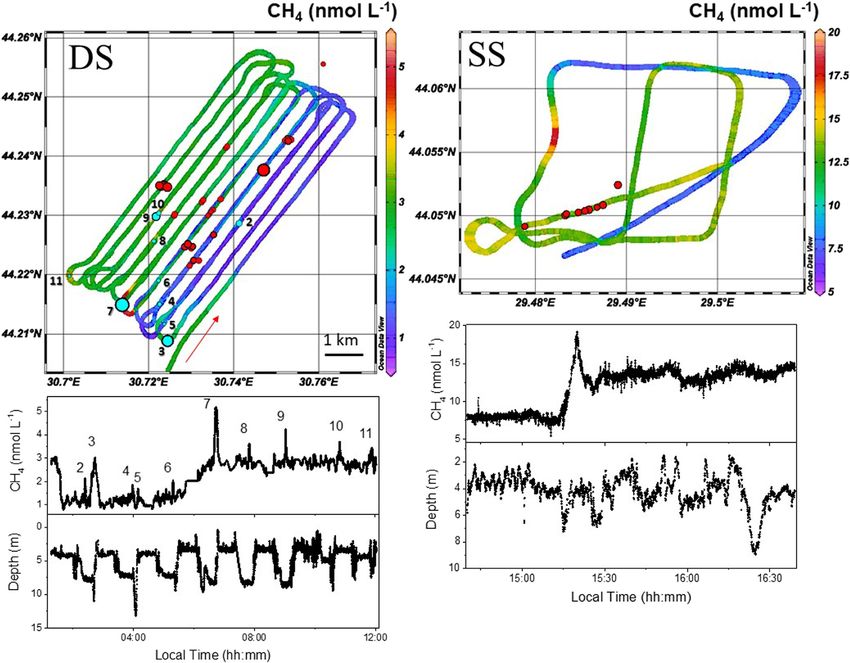
Grilli et al.                                                                                                          Methane Seafloor Emissions Black Sea

                                            dissolved methane in the water column, especially in stratified water masses like in the
                                            Black Sea.
                                            Keywords: dissolved gas, methane, black sea, in situ measurements, gas seepages, instrumental inter-comparison

INTRODUCTION                                                                       of method depends mainly on the methane concentration and the
                                                                                   sample volume available. Although the PT-GC requires a larger
Methane is a key climate-relevant trace gas widely encountered in                  volume of water than the HS-GC (>100 ml vs 5–20 ml), it
seawater (Reeburgh, 2007; Etiope, 2012; Myhre et al., 2016;                        provides a sub-nmol L−1 detection limit, whereas that of the
Saunois et al., 2017; Weber et al., 2019). Its distribution in the                 HS technique is usually around few nmol L−1.
water column is highly heterogeneous, both horizontally and                            Despite the reliability of laboratory measurements, in situ
vertically. In the open ocean, dissolved methane concentrations                    measurements are increasingly needed for both long-term
are at level of nmol per litre (10–9 mol L−1), and usually at higher               monitoring through remote sensing and observatory, and
concentrations within the near-surface most-ventilated and                         high-resolution coverage of large areas of methane emissions.
most-oxygenated water (Karl et al., 2008; Repeta et al., 2016).                    The most commonly encountered instruments for in situ
However, very high concentrations of methane can also be found                     methane concentration measurement are optical and chemical
in bottom waters at coastal, shelf and margin settings                             sensors (Marinaro et al., 2004; Faure et al., 2006; Krabbenhoeft
characterized by widespread gas seeps discharging fluids at the                     et al., 2010; Schmidt et al., 2013), as well as optical spectrometers
seafloor (e.g., Reeburgh et al., 1991; Borges et al., 2016; Mau et al.,             (e.g. Chua et al., 2016; Boulart et al., 2017; Grilli et al., 2018;
2017; Ruffine et al., 2018). In such settings, the water column is                  Hartmann et al., 2018; Yuan et al., 2020). Their measurement
considered as a sink for methane in which it is transported at                     range spans from few tens of nmol L−1 to hundreds of μmol L−1,
short (meters) and medium (kilometers) distances, degraded or                      and they can be used up to hundreds of meters water depth.
transferred into other earth compartments like the atmosphere.                         Furthermore, anoxic environments receiving huge inputs of
The dynamic of methane in the water column is complex and                          organic matter provide favourable conditions for the production
depends on the properties of the water mass: physical conditions                   and preservation of high concentrations of methane, and the
such as currents, layer thickness, temperature, ventilation/                       Black Sea is well known for being a typical example (e.g. Kessler
exchange with the atmosphere, chemical conditions that                             et al., 2006a; Pape et al., 2008; Reeburgh et al., 1991, 2006).
control its redox state (e.g. hypoxic/anoxic conditions) and                       Indeed, it represents the largest thick and permanently anoxic
biological activity that might oxidize or even produce methane                     and sulfidic basin on earth, in which methane is discharged
in the water column (Solomon et al., 2009; Shakhova et al., 2014;                  abundantly through seeps widely distributed on the shelf and
Weinstein et al., 2016; Garcia-Tigreros and Kessler, 2018). The                    slope, typically at the rim of the gas hydrate stability zone and
multiple factors involved in methane transport and                                 from mud volcanoes in the deep basins (Artemov et al., 2019). In
transformation explain why the fate of this compound in the                        the anoxic waters below ∼100 m water depth, methane
dissolved state is still difficult to capture in the field. However, in a            concentrations can reach values of more than 10 µmol L−1 in
progressively warming climate, in-depth knowledge of the fate of                   contrast to the nmol L−1 level observed in the surface layer (e.g.
methane is essential, as emissions are expected to increase,                       Schmale et al., 2010).
particularly from continental shelves and margins due to                               The anoxic layer is successively superimposed by an
eutrophication,       permafrost       thaw      and    gas   hydrate              intermediate suboxic- and an oxic-layer, leading to a distinct
destabilization (Westbrook et al., 2009; Naqvi et al., 2010;                       vertical stratification of the water column with limited chemical
James et al., 2016; Riboulot et al., 2018). Accordingly,                           exchanges of redox-sensitive species (Capet et al., 2016; Özsoy
campaigns of time series and worldwide measurements are                            and Ünlüata, 1997; Stanev et al., 2018, 2019). The total amount of
indispensable to capture the time evolution of methane.                            dissolved methane stored in the Black Sea is estimated at ∼96 Tg
    The methane concentration in seawater can be measured                          (Reeburgh et al., 1991) with the anoxic water layer being more
either in the laboratory from previously collected water                           charged (∼72 Tg) than the others (Artemov et al., 2019).
samples or in situ using specific sensors and analyzers.                                Previous Black Sea methane studies have highlighted a variable
Laboratory measurements consist of determining the methane                         vertical concentration distribution (McGinnis et al., 2006;
concentration either by headspace (HS) or purge-and-trap (PT)                      Schmale et al., 2010; Sovga et al., 2008), with increasing values
methods coupled with gas chromatography (GC) (Lammers and                          while going from the oxic into the anoxic water layer. So, methane
Suess, 1994; Tsurushima et al., 1999; Donval and Guyader, 2017;                    concentrations up to 12 nmol L−1 were measured in the oxic
Wilson et al., 2018). HS-GC is based on the analysis of the gas                    layer, and in some areas, the sea surface was oversaturated in
phase in equilibrium with the seawater sample; it is easy to                       methane with respect to the atmosphere (Malakhova et al., 2010;
perform and could also be implemented in the field. The PT-                         Reeburgh et al., 1991). Concentrations reaching a few μmol L−1
GC method requires a more sophisticated installation in which                      were measured within the suboxic layer, and up to >10 μmol L−1
the originally dissolved methane is extracted by flowing a carrier                  in the anoxic water mass (Kessler et al., 2006a; Reeburgh et al.,
gas throughout the seawater sample, followed by its entrapment                     2006), where the concentration variations are much less
in a cooled material, frequently active carbon or silica. The choice               pronounced.

Frontiers in Earth Science | www.frontiersin.org                               2                                        July 2021 | Volume 9 | Article 626372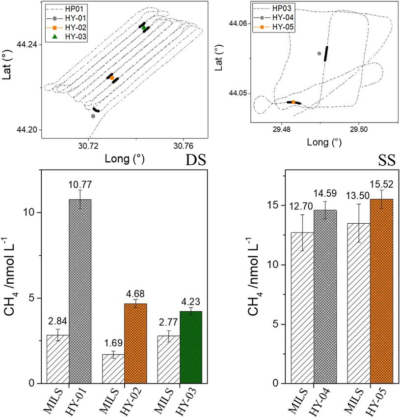
Grilli et al.                                                                                               Methane Seafloor Emissions Black Sea

    Although today we are relatively confident that the methane            equipped with dynamic positioning, inter-comparisons on
originating from the Black Sea sediments is not a significant              dissolved methane measurements remain challenging.
source accounting for the atmospheric CH4 budget of the region,
its transfer mechanisms from the seafloor through the three                The Study Areas
aforementioned water layers and seldom to the atmosphere                  The survey was performed on board of the R/V Mare Nigrum,
still remain unknown and controversial in the scientific                   operated by GeoEcoMar Romania, in April 2019 at two shallow
community (Schmale et al., 2005; McGinnis et al., 2006).                  sites in the Black Sea Romania territorial water. Over a period of
Depending on the investigated area, different sources of                  5 days (3–7 April), we surveyed an area of ∼ 12.5 km2 at the
discharged methane can be identified: deep hydrocarbon-                    deeper site (44.233°N, 30.737°E, 100-km long survey), with water
reservoirs, gas-hydrate destabilization, shallow methanogenesis           depths between 110 and 128 m, and ∼ 3.5 km2 at the shallower
within the sediments, and even methanogenesis in the water                site (44.057°N, 29.491°E, 19-km long survey), with water depths
column (Reeburgh et al., 1991; Kessler et al., 2006b). The                between 53 and 58 m (Figure 1).
contribution of these sources can be very asymmetric, and                     At the deeper site, water temperature and electrical
Kessler et al. (2006b) showed that the major methane inputs               conductivity were on average 9.5°C and 18.5 mS cm−1 at the
to the Black Sea water column are discharges from seeps and               sea surface, and 9.0°C and 20.5 mS cm−1 near the seafloor. At
diagenesis within the sediments.                                          the shallower site, temperature and electrical conductivity were
    Despite several European and national Black Sea Projects (e.g.,       9.5°C and 18 mS cm−1 at the sea surface and 8.0°C and
CRIMEA, METROL, MSM34 cruise by Geomar in 2013–2014                       18.5 mS cm−1 at the seafloor. The deeper site showed an
(EU project MIDAS), Ghass cruise by Ifremer in 2015 (ANR                  oxycline between 60 and 80 m water depth, while the
project Blame) and many other German research cruises with                concentration of dissolved oxygen near the seafloor at the
R/V Meteor and R/V Maria S. Merian), the distribution and fate            shallower site was 17% lower than at the surface
of methane emissions in Romanian waters are still not fully               (360 mmol L−1) (CTD, Conductivity, Temperature and Depth,
constrained (Ghass, 2015; MSM34, 2014; Riboulot et al., 2018).            data are reported in the Supplementary Datasheet S1).
The objective of this study is to present insights from the
dissolved methane distribution in the water column from two               Description of the Surveys
shallow water emission sites (∼55 m water depth, hereafter                Two near-surface horizontal profile surveys (HP01, mean depth
referred to as “shallower site” and ∼120 m water depth,                   5.2 m, min 0.4 m, max 18 m, and HP03, mean depth 4.2 m, min
hereafter referred to as “deeper site”) in the Romanian sector            1.5 m, max 9 m) on dissolved CH4 were conducted. HP01 was
of the Black Sea using a multi-technique approach. High-                  performed for 11 h at the deeper site on April 4th and is
resolution, horizontal and vertical profiles of dissolved                  composed of ten parallel ∼5.5-km long lines spaced by
methane concentration obtained from in situ measurements                  ∼260 m, for a total surface area of ∼ 12.5 km2. HP03 was a
are reported and correlated to hydro-acoustic studies of gas              2-h long survey at the shallower site performed on the April
bubbles. A detailed analysis of the results of the measurement            6th, covering an area of ∼3.5 km2 (see Figure 1). During these two
systems is presented, and it emphasises the need to develop               surveys, the MILS and METS sensors were deployed
reliable and standardized protocols for in situ measurement of            simultaneously. The MILS probe was configured to improve
dissolved CH4. The two sites are then compared and the dissolved          the sensitivity of the measurements, by minimizing the flow of
methane distribution in the water column discussed.                       carrier gas (see the method description below for further details).
                                                                          This decreased the dynamic range of the measurement, while
                                                                          increasing the precision at low concentrations, to the detriment of
MATERIALS AND METHODS                                                     a slightly longer response time (t90 of 30 s, corresponding to 75 m
                                                                          resolution at the highest speed of 2.5 m s−1 reached during the
Recent previous studies on the distribution of dissolved CH4 at a         surveys).
seepage site have highlighted the need for high-resolution                    Vertical profiles (VPs) with the MILS and METS sensors were
methane concentration measurements to assess the extent of                performed at different locations at the two sites. Because of the
the influence area of a bubble plume and map the spatial                   lacking in dynamical positioning, the vessel was located in the
concentration variability (Jansson et al., 2019b). In this                vicinity of a flare (hydroacoustic anomalies in echosounder
respect, the fast response membrane inlet laser spectrometer              records attributed to the presence of gas bubbles) or a cluster
(MILS) prototype (t90 < 30 s, Grilli et al., 2018) is well-suited.        of flares, and down- and up-casts were performed. It should be
To better appreciate its performances, comparison was made with           noticed that because of the strong dependency of the METS
the Franatech METS sensor and against a standard method                   sensor to dissolved oxygen content and change in hydrostatic
consisting of sampling with Niskin bottles followed by PT and             pressure, the recorded vertical profiles are not reported in
HS analysis in the laboratory. This multi-technique approach              this work.
identifies the advantages and drawbacks of the different methods,              Hydro-casts (HYs) for discrete water sampling were
revealing weaknesses and possible artifacts in the measurements,          conducted at different time with respect to in situ
while making the dataset more robust for the comparison                   measurements. The locations should have been the same as
between the two locations reported in the discussion section.             the in situ measurements, but this has proven to be
It should be noticed here that, since the research vessel was not         challenging due to the lack of dynamical positioning of the vessel.

Frontiers in Earth Science | www.frontiersin.org                      3                                      July 2021 | Volume 9 | Article 626372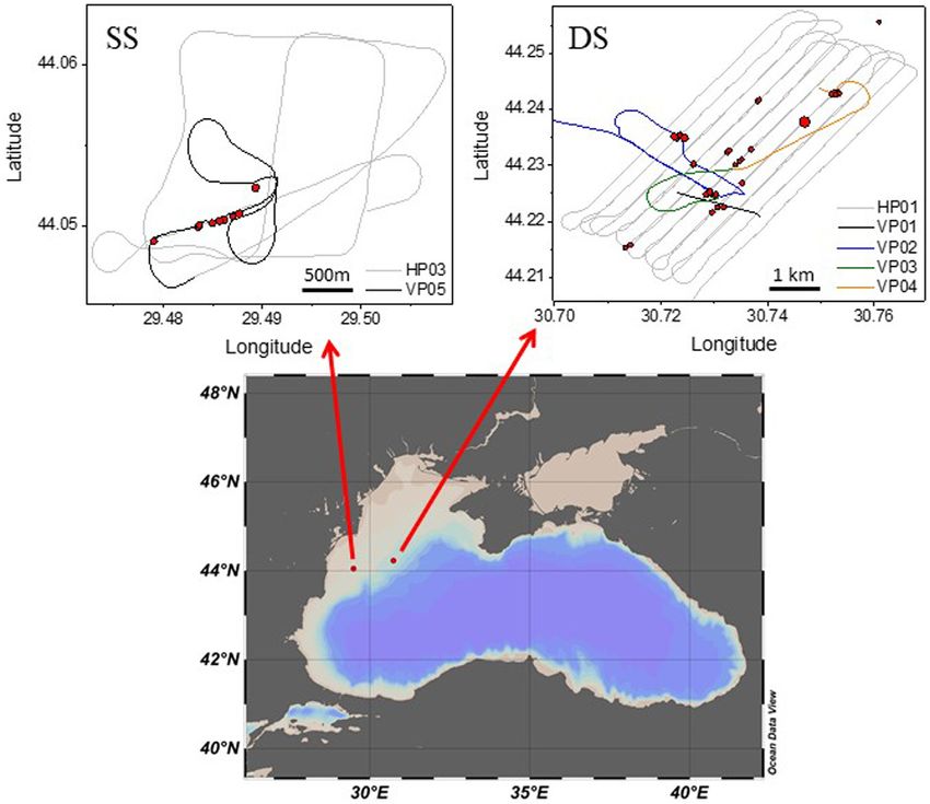
Grilli et al.                                                                                                                                Methane Seafloor Emissions Black Sea

  FIGURE 1 | Maps of the survey areas. At the bottom a large map of the Black Sea, and at the top two maps of the shallower site (SS, left) and deeper site (DS,
  right) with the trajectories of the vessel for the profiles of interest for this work. VP are vertical and HP are horizontal near-surface profiles in the water. During the vertical
  profiles the position of the vessel was drifting due to water current. Red dots are the locations of flares identified during the survey by the echosounder, with the size
  proportional to the strength estimated from the acoustic signature.

The Acoustic Method                                                                            been accepted as an efficient approach to identify submarine gas
During the cruise, a 70 kHz split beam echosounder (Simrad                                     flares. The method has been described in detail in e.g. Greinert
EK80 with ES70 transducer) was used to hydro-acoustically                                      et al. (2010) and Veloso et al. (2015).
detect and locate bubble releasing methane seeps. With an
opening angle of 18°, it has a footprint at the seabed of ∼22 m
and ∼48 m diameter at 55 m and 120 m water depths,                                             The Membrane Inlet Laser Spectrometer in
respectively. The pulse length was set to 0.256 ms over the                                    situ Sensor
entire cruise. This turned out to be suitable for the shallower                                A membrane inlet laser spectrometer (MILS) prototype allowing
site, while for the deeper site the noise level remained visibly                               the combination of fast response and in situ dissolved methane
higher. However, since this noise level was acceptable, for a better                           measurements was used. The instrument relies on a patent-based
inter-comparability between the two study sites, the pulse length                              membrane extraction system (Triest et al., 2017). It is described in
was unchanged for both surveys. At an average vessel speed of                                  detail in a previously published paper (Grilli et al., 2018), where a
∼2 m s−1, the distance between two pings was around 32 cm                                      laboratory comparison with measurements of discrete water
(14 cm) for 120 m (55 m) water depth at a ping rate of 0.16 s                                  samples at different water temperatures and salinities was
(0.07 s). To obtain precise backscatter values for the bubble                                  conducted. It was deployed successfully during two campaigns,
quantification method, the echosounder was calibrated prior to                                  over a methane seepage area in western Svalbard in 2015 (Jansson
the cruise with a 38.5 mm Tungsten sphere for the applied pulse                                et al., 2019b), and at Lake Kivu in Rwanda in March 2018 (Grilli
length (MacLennan and Svellingen, 1989).                                                       et al., 2020). The instrument allows a dynamic range from a few
    The idea to detect gas seepage locations using echo-sounding                               nmol L−1 up to a few μmol L−1. The MILS was powered by a
techniques was adopted from a series of former studies and has                                 battery pack (SeaCell, STR Subsea Technology and Rentals) and

Frontiers in Earth Science | www.frontiersin.org                                           4                                                  July 2021 | Volume 9 | Article 626372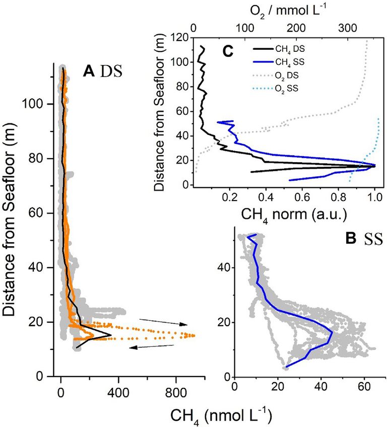
Grilli et al.                                                                                                   Methane Seafloor Emissions Black Sea

deployed together with a CTD SBE 911plus (Seabird) for                      Where Ai and Bi are empirical parameters from Wiesenburg and
measuring temperature, conductivity and water depth.                        Guinasso. (1979).
    Because of the dynamic and fast profiling capability of the                 The solubility coefficients need to be corrected for local pressure
instrument, the spatial and temporal synchronization of                     P (Pa) at the sampling water depth (sum of hydrostatic and
measurements needs particular attention. For this, a first                   atmospheric pressure), using the following equation (Weiss, 1974):
dynamic correction of the time-lag due to the flushing time                                                       (1−P)vCH
                                                                                                                        4
(the time it takes the gas sample to go from the membrane                                           K(P)  Ke       RT
                                                                                                                                 ,                   (3)
extraction system into the measurement cell) was applied. By
knowing the total gas flow (sum of the carrier gas plus the dry and          where R  8.31446 J mol−1 K−1 is the ideal gas constant, and νCH4
wet gas permeating the membrane) and the volume of the gas line             is the partial molar volume (cm3 mol−1) of CH4 calculated from
between the extraction system and the measurement cell, this                Rettich et al. (1981).
time lag was calculated and varied between 15 and 60 s during the               Calibration of the instrument was performed in the laboratory
campaign (depending on the total gas flow). The instrument                   using the calibration system described in Grilli et al. (2018).
response time is related to the time necessary to replace the gas           Experiments were performed at atmospheric pressure for
inside the measurement cell; it depends on the measurement cell             different water conditions (temperature from 5 to 25°C, and
volume (∼20 cm3 at standard temperature and pressure), the                  salinity from 0 to 30.5 g/kg) and at different concentrations of
working pressure (20 mbar) and the total gas flow. This                      CH4 (0–1,000 ppm). The gas mixtures were obtained using two
parameter can as well be calculated and it varied between 8                 mass flow controllers (Bronkhorst, EL-FLOW) and mixing zero
and 30 s during the campaign. Both time-lag and response time               air (ALPHAGAZ 2, Air Liquide) with synthetic air containing
are affected by the total gas flow (Grilli et al., 2018). With the           CH4 (8920 Labline, 1,000 ppm of CH4 in air, Messer).
instrument towed behind the vessel, the distance between the
instrument and the ship also varies as function of the ship speed           The Commercial Sensor Franatech
and water depth of the sensor. Instrument location was therefore            A Franatech METS sensor was used to measure anomalies in a
dynamically corrected simulating the mooring of our sensor                  concentration of dissolved methane in water. The measurement
using the “Mooring Design and Dynamics” matlab routine                      principle is based on a SnO2 semiconductor detector (Seiyama
(Dewey, 1999). This dynamic correction allows to apply a time               et al., 1962) working at ∼500°C (Ippommatsu et al., 1990). Its
(and therefore a position) correction of the sensor which ranged            principles can be summarized as follows: first, oxygen (O2) is
from a few seconds and a few meters at the sea surface and at               absorbed on the SnO2, then, the dissolved CH4 diffuses through a
minimum speed, up to 100 s when the system was towed at 100 m               membrane to the measurement cell and interacts with O2 molecules,
water depth. This corresponds to maximum horizontal correction              causing their desorption and increasing the conductivity of the SnO2
of ∼80 m, since typical ship speed during vertical profiles was              material. This technology is however known for its lack in gas
∼0.8 m/s. Water currents were neglected for this position                   selectivity and its dependency on the amount of O2 present in the
correction. The vessel position was provided by a Garmin GPS                measured environment (Boulart et al., 2010; Chua et al., 2016). The
18x, with an accuracy of 15 m (1σ).                                         METS sensor can be operated at water depths down to 4,000 m and
    Measured concentrations are reported in mixing ratio with               temperature ranging between 2°C and 20°C. Prior to its deployment,
respect to the total dissolved gas pressure, which is assumed to be         the sensor was calibrated by the manufacturer (in February 2019) at
1 atm for this setting. Therefore, a value of partial pressure, pCH4,       atmospheric pressure and methane concentrations ranging between
in the gas mixture can be retrieved, which is then converted into           100 nmol L−1 and 40 µmol L−1. Although the sensor can be operated
dissolved methane concentrations, CCH4, expressed in mol per                over a larger methane concentration range, the manufacturer
liter of water. This conversion is performed by considering the             calibrated the sensor in a narrower range in order to preserve its
solubility of the gas in the water under given physical conditions          linear response (Franatech Pers. Comm.).
as well as its fugacity. CCH4 is related to the pCH4 through the
following equation:                                                         The Discrete Water Measurements
                                                                            Discrete water sampling was conducted using a CTD-rosette with 16
                   CCH4  K(T, S, P)pCH4 φCH4 (T, P),            (1)        Niskin sampling bottles (8 L), a SBE 911plus CTD (Seabird), an
                                                                            altimeter (Teledyne Benthos PSA 916), and an oxygen optode
where φCH4 is the fugacity coefficient (assumed to be one in this
                                                                            (Aanderaa Optode 4831F). The sensors were connected through
case) and K is the solubility coefficient, i.e. the ratio between the
                                                                            telemetry for real-time monitoring of the water depth of the
dissolved methane concentration and its fugacity. The solubility
                                                                            assembly. This allowed to adjust the sampling strategy during the
coefficient K (mol L−1 atm−1) of CH4 as a function of temperature
                                                                            profile according to the anomalies recorded by the echosounder. The
T (K) and salinity S (g/kg) is calculated using the following
                                                                            Niskin bottles were sampled during the up-cast, and water
equation:
                                                                            subsampling was performed onboard for laboratory gas analysis
                           100            T               T                 (both PT and HS). For all the samples, a few mg of sodium azide
     ln(K)  A1 + A2           + A3 ln  + SB1 + B2                   (NaN3) were added to the vials and glass bulbs before adding the water
                            T            100             100
                                                                            sample. Filled vials for HS analysis were then stored upside down.
                          T 2
                + B3         ,                                (2)            The samples were analyzed by two different techniques: the purge
                         100                                                and trap (PT) and the headspace (HS) techniques. These methods

Frontiers in Earth Science | www.frontiersin.org                        5                                           July 2021 | Volume 9 | Article 626372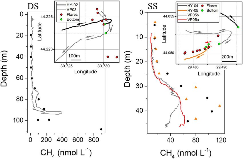
Grilli et al. Methane Seafloor Emissions Black Sea
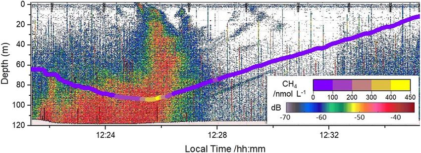
FIGURE 2 | Qualitative comparison between the time series from the continuous concentration of dissolved methane measured by MILS (colored line) and the
acoustic signal from the echosounder (colored background). The data are plotted against local time. The data are from the VP03 profile performed on April 5th at the
deeper site (44.224°N, 30.730°E).
have already been compared and validated in the laboratory (Donval validating the finds on the dissolved methane distribution in the
and Guyader, 2017). The PT method used here is based on water column at the studied sites. This data validation is
Swinnerton et al. (1968) and modified by Luc Charlou et al. important for comparing the distribution of dissolved methane
(1988). Briefly, 125 ml glass bulbs devoted to the analysis of at the two locations as reported in the discussion section.
methane by PT method were used. The bulbs were overflowed
with twice the volume of seawater. Particular care was taken to
exclude air bubbles during sampling and avoid contamination.
Qualitative Comparison of Echosounder
Once in the laboratory, CH4 was stripped from seawater for 8 min Data and Membrane Inlet Laser
using helium as carrier gas (quality 99.9995%), trapped on activated Spectrometer
charcoal at −80°C, and detected and quantified with a flame ionization On the echogram, large areas of high backscatter (>−30 dB) of a
detector after separation on a packed column (GC Agilent 7890A/ flare-like shape have been identified as methane gas seeping
column Porapak Q 2 m). The calibration was performed by injection areas (Figure 2, color-coded in orange to red). Broader high
of gas standards containing 108 ppm of CH4 in air ±5% (Restek). The backscatter areas are related to vessel movement. In our case, the
limit of detection was 0.03 nmol L−1, the precision based on five ship remained over the methane seep location for some time and
replicates from the same rosette bottle was within ±2% (±1σ), while as the echogram displays backscatter over time, the seepage area
the accuracy corresponds to that of the gas standards (±5%). The HS widens. During the cruise, 36 and 13 gas emissions in the deeper
method (Donval et al., 2008; Donval and Guyader, 2017) was and shallower site, respectively, were identified from the 70 kHz
performed on 10 ml vials by analyzing the composition of the echosounder data. The signal produced by the scattering of the
headspace in equilibrium with the water. At the beginning of the acoustic wave by the gas bubbles provides only qualitative
cruise, the vials were flushed with zero air (Alphagaz 2, Air Liquide) to information about the distribution of dissolved CH4 in the
avoid introducing methane into the initial gas phase. With a gas tight water column. This is due to the fact that gas bubbles shrink
syringe, 5 ml of seawater were transferred into the vial while a second and change their chemical composition during their rise
needle was introduced to keep the pressure close to atmospheric through the water column, and that free bubble-forming gas
pressure inside the vial. The analysis was performed by means of a is mobile whereas dissolved methane is more stationary.
headspace sampler connected to the same GC unit used for the PT Therefore, a quantitative analysis would require different
method. The limit of detection was 5 nmol L−1 and the precision was assumptions on the initial bubble size distribution, the
≤10% for concentrations below 100 nmol L−1, and ≤5% for higher bubble rising speed and the gas exchange ratio between the
concentration (±1σ). Further details in the comparison between the two phases. Results from the quantitative analysis of the acoustic
results of two methods can be found in the Supplementary signal is beyond the scope of this paper, and will be the subject of
Datasheet S1. another study. Here, an example of the qualitative comparison
between the acoustic signal and the dissolved CH4
concentrations from MILS is reported in Figure 2 for the
RESULTS VP03 profile performed on April 5th at the deeper location
(44.224° N, 30.730° E). The concentrations of dissolved methane
Inter-Comparison Between the Techniques determined by MILS were dynamically corrected for the
In this section we compare results from different techniques with position of the instrument with respect to the vessel. This
the aim of testing the reliability of the measurements, identifying correction allows to synchronize/match the two time-series,
possible artefacts or weaknesses of each technique used, and accounting for the fact that the echosounder passed over a
Frontiers in Earth Science | www.frontiersin.org 6 July 2021 | Volume 9 | Article 626372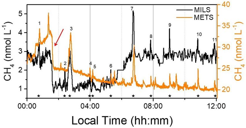
Grilli et al.                                                                                                           Methane Seafloor Emissions Black Sea

                                                                                    concentrations obtained with the MILS. Previous field studies
                                                                                    have shown significant differences between measurements of
                                                                                    discrete water samples of seawater methane concentration from
                                                                                    well-proven laboratory methods and the METS outputs (Heeschen
                                                                                    et al., 2005; Newman et al., 2008). This has led Heeschen et al.
                                                                                    (2005) to interpret their METS in situ measurements in a
                                                                                    qualitative way. Here, the differences observed between the
                                                                                    MILS and the METS measurements may be explained by: 1)
                                                                                    the fact that the METS sensor was used below the calibration
                                                                                    range (100 nmol L−1–40 μmol L−1 at atmospheric pressure)
                                                                                    certified by the manufacturer and therefore it cannot provide
                                                                                    reliable quantitative measurements at the sea surface; 2) the
  FIGURE 3 | Comparison between the dissolved methane                               METS suffers from dependency to hydrostatic pressure, salinity
  measurements from the MILS and the METS sensor which were deployed                and oxygen content (Newman et al., 2008), which makes near-
  simultaneously during the 12 h HP01 survey. The red arrow indicates a sharp       surface horizontal profile also challenging. Moreover, the wide
  concentration decrease observed by both instruments. Well localized               drifts observed during this 12 h continuous near-surface profile
  peaks of dissolved CH4 were observed by both instruments (main identified
  methane peaks are numbered and identified by the stars at the bottom).
                                                                                    (Figure 3) can be explained by the fact that small height changes in
                                                                                    near-surface depth lead to large relative changes in hydrostatic
                                                                                    pressure that considerably affect the sensor response. Despite the
                                                                                    large discrepancy on the methane concentration from the METS
target area prior to the towed MILS. A more detailed figure                          sensor, both in situ instruments agreed on the presence of highly
reporting original and synchronised data can be found in                            localized peaks of CH4 at the sea surface. The METS sensor, even
the Supplementary Datasheet S1.                                                     when it is used outside the calibration range and under severe
   In this inter-comparison, one should consider that the MILS                      conditions (changing oxygen concentration that affect its detection
probe is measuring a specific location behind the vessel, while                      system) can provide valuable qualitative information on the
acoustic data has a larger footprint on the seafloor as well as in the               location of dissolved methane concentration spots. Further
water column. This may induce discrepancy between the two                           laboratory tests, together with deployment at deeper water
signals, for instance in the case of a bubble plume located a few                   depth within the anoxic layer, would be required to provide a
tens of meters on a side of the MILS instrument that would be                       thorough assessment of the sensor for quantitative and reliable
spotted acoustically but not observed by the MILS (this could be                    dissolved methane measurements.
the case for the signature at 12:22 local time in Figure 2, more                        Eleven well localized dissolved CH4 peaks (numerated and marked
visible in Supplementary Figure S1-3). The results may inverse if                   with stars in Figure 3) were identified during the horizontal profile
water enriched in CH4 (by a bubble plume that is outside the                        HP01 and are discussed in the next section. Furthermore, the sharp
acoustic lobe) is laterally transported by currents. This may be the                concentration decrease recorded at 01:35 local time (highlighted in
case for the increase in dissolved CH4 at 12:28 local time (visible                 Figure 3 by the red arrow and also visible in the 2D colored map graph
in Supplementary Figure S1-3) that was observed by the MILS                         of the dissolved methane concentrations measured by the MILS
sensor without the corresponding acoustic signal.                                   instrument and reported in Figure 4) that could have been
   Despite its evident limitations, this comparison allowed us to                   associated with a possible instrumental (MILS) drift, was
verify the qualitative agreements between these two datasets and                    confirmed as a real signal since observed by both in situ sensors.
validate the dynamic correction of the position of the MILS probe
with respect to the vessel during the profiles.
                                                                                    Membrane Inlet Laser Spectrometer Vs
                                                                                    Measurements of Discrete Water Samples
Comparison Between the Two in situ                                                  at the Deeper and Shallower Sites
Instruments                                                                         Comparison on Vertical Profiles
For comparison, the MILS and the METS sensor were deployed                          The size of the MILS prototype did not allow to be mounted on the
simultaneously during the vertical and horizontal profiles.                          CTD for continuous in situ measurements simultaneous to discrete
However, due to dependency of the METS sensor to the                                water sampling. For this reason, measurements with the MILS
hydrostatic pressure, salinity and oxygen (Newman et al., 2008),                    probe and discrete water samplings could not be conducted
this comparison only focus on the 12-h long horizontal profile                       simultaneously. Moreover, because the research vessel was not
(HP01). The profile was conducted at ∼5 m depth, and the water                       equipped with dynamic positioning, inter-comparisons on
inlets of the two sensors were ∼10 cm distance from each other.                     dissolved methane measurements were challenging. As
The resulting profiles used for comparison are reported in                           mentioned above, due to the high spatial variability of dissolved
Figure 3. One can clearly see that most of the peaks in                             methane relative to the location and intensity of bubble streams, a
methane concentration for both instruments agree with each                          few hundreds or even a few tens of meters could be significant for
other. However, the methane concentrations measured by the                          correctly reproducing the same spatial distribution of dissolved
METS are more than one order magnitude higher than the                              CH4. However, we identified a few vertical profiles at the shallower

Frontiers in Earth Science | www.frontiersin.org                                7                                        July 2021 | Volume 9 | Article 626372
Grilli et al. Methane Seafloor Emissions Black Sea FIGURE 4 | 2D surface dissolved methane distribution (color map) at the deeper (DS, left) and shallower (SS, right) site. Both surveys were conducted near surface. The thickness of the color map (∼60 m) was chosen accordingly to the 2σ accuracy of the GPS positioning. Red arrows indicate the time direction. Red and light- blue dots show the locations of the flares (echosounder) and surface dissolved CH4 (MILS) peaks, respectively, both with the size proportional to the estimated intensity. Peak 1 is only visible in Figure 6, because it is located at a southern position with respect to the performed grid. At the bottom, the time series of the data together with the water depth information. Localized peaks of dissolved CH4 were observed at certain locations, which seems uncorrelated with the flare locations. and deeper sites, where the position of the MILS was relatively close with respect to the measurement from discrete water sample to the hydro-casts (HYs) for discrete water sampling. These profiles analysis. This may be due to the strong spatial variability caused are reported in Figure 5. The trajectories of the vessel during the by the ascent of the multiple methane bubbles of variable size measurements are shown in the inserts. The arrows indicate the and trajectory within the water column, or by an unidentified time direction of the deployment, while the location of the bottom bias in either the MILS or discrete sampling methods. Our of the profile is indicated by green dots. The VP03 profile results highlight the limitations of current in situ performed by the MILS sensor started with the probe at 60 m instrumentation and laboratory measurement techniques. water depth, and it went first down to 93 m, and then back up to Nevertheless, a larger number of measurements together with the surface. Red dots are the positions of the flares identified during improved position maintaining or simultaneous deployment of the campaign. For discrete water sample measurements average the in situ instruments and Niskin bottle sampler would have values between the PT and HS analysis were used. Dissimilarities been required for a finer comparison of the two methods. between the two techniques at the two sites ranged from Further information on this comparison can be found in 8 nmol L−1 (0–70 m water depth) to 86 nmol L−1 (>70 m the Supplementary Datasheet S1. water depth) at the deeper site, and from 8 nmol L−1 (0–25 m water depth) to 62 nmol L−1 (>25 m water depth) at the Comparison on Near-Surface Measurements shallower site. At the shallower site, the MILS curves MILS continuous sea-surface measurements were compared with systematically show lower concentrations of dissolved CH4 the results from discrete water sampling performed during the Frontiers in Earth Science | www.frontiersin.org 8 July 2021 | Volume 9 | Article 626372
Grilli et al.                                                                                                                      Methane Seafloor Emissions Black Sea

  FIGURE 5 | Comparison between the dissolved methane measurements from MILS (VP) and discrete water sample (HY) techniques at the two sites (average
  concentrations between PT and HS methods are reported). The inserts show the trajectory of the vessel during the measurements, which were performed at different
  time and without dynamic positioning of the vessel. Red circles in the maps report the location of the flares identified from the acoustic survey. Arrows in the inserts
  represent the time direction of the measurement, and green dots the location of the bottom of the profile.

TABLE 1 | Data used in Figure 6 for the deeper and shallower site. MILS (Membrane inlet laser spectrometer) data are an average from measurements which were closest to
the discrete water sampling (HY) locations. HY data are averages between the PT and HS analysis. Water depths and estimated accuracies of the measurements are
also reported.

                         —                                          MILS                                                                    HY
—                        —             Depth/m             CH4/nmol L−1             Accuracy (12%)             Depth/m            CH4/nmol L−1             Accuracy (5%)

Deeper site            HY-01               5.9                  2.84                      0.34                    10.4                 10.77                     0.54
                       HY-02               5.2                  1.69                      0.20                    19.4                  4.68                     0.23
                       HY-03               4.6                  2.77                      0.33                     8.6                  4.23                     0.21
—                       —                  —                     —                         —                       —                     —                        —
Shallower site         HY-04               5.0                 12.70                      1.52                     5.0                 14.59                     0.73
                       HY-05               3.6                 13.50                      1.62                     3.9                 15.52                     0.78

HYs. The results from the shallowest measurements of the HY                                  The comparison between MILS and measurements of discrete
profiles were used (average concentrations between the PT and                             water samples at the shallower site (HY-04 and HY-05) shows a
HS method; depths and accuracies of the measurements are                                 discrepancy of ∼13% (([CH4]MILS - [CH4]HY)/[CH4]HY), which
reported in Table 1), and compared against the closest data                              lies within the accuracy of the measurements, as reported in
from the MILS sensor. In the two maps of Figure 6, the                                   Table 1. At the deeper site, the differences are larger, with 34%
trajectories during the MILS survey and the location of the                              discrepancy for the HY-03 and even larger for HY-01 and HY-02.
near-surface discrete water sampling (HYs) are reported for                              Different hypotheses can explain these discrepancies. As
the deeper and shallower site. The concentration of dissolved                            mentioned above, the measurements were not conducted at
methane measured by MILS closest to the locations of the HYs                             the same time. At the shallower location, HP03, HY-04, HY-
were selected and highlighted with thick black lines. The selected                       05 were conducted on the same day (April 6th), while the
MILS data were averaged at each location, and reported in the bar                        measurements at the deeper site were spread over two and
graph of Figure 6 together with the results from the                                     half days (April 3rd to 5th). Thus 1) The spatio-temporal
concentrations in dissolved methane by the analysis of discrete                          variability of dissolved CH4 at the sea surface can be affected
water samples.                                                                           by water currents producing different distribution patterns as well
    The location of the HY-02 and HY-03 measurements lies between                        as meteorological conditions (change in wind direction or speed,
two horizontal profile lines, therefore data from both lines were                         humidity, water temperature, etc.) (Shakhova et al., 2014) that
selected and averaged. HY-05 was very close to the horizontal profile                     modify gas exchange/equilibration with the atmosphere and
trajectories, while for HY-01 and HY-04 the closest dissolved CH4                        degassing activities at the seafloor. Although, this last
MILS data were 300 and 140 m away, respectively.                                         hypothesis would require significant changes in meteorological

Frontiers in Earth Science | www.frontiersin.org                                     9                                               July 2021 | Volume 9 | Article 626372
Grilli et al. Methane Seafloor Emissions Black Sea
FIGURE 6 | Bottom: Comparison between near-surface water depth measurements made by the MILS sensor and the analysis of discrete samples (HY) at the
deeper (DS, left) and shallower (SS, right) site. Data from discrete samples are reported as the average between the two analytical techniques used (PT and HS). Maps
with locations are reported at the top, with the trajectories of the MILS surveys (dotted lines) and locations of the near sea surface sampling of the HYs. In thick black lines
are the selected dissolved CH4 MILS data closest to the discrete sampling locations which were averaged and used for the comparison.
conditions in order to explain the reported discrepancies; 2) the For the deeper site, a total of four down- and up-casts (VP01, 02,
discrepancy could be due to the analytical techniques itself. The 03, and 04) were used, whereas for the shallower location, the
MILS measurements seem to be systematically lower than the vertical profile VP05, composed of a series of seven down- and
measurements of discrete water samples. Apart from the HY-01 up-casts over the seepage area was used. The 2-m average curves
location where a 7.9 nmol L−1 difference was found, for the other are in black and blue for the deeper and shallower sites,
locations the offset between the two techniques is ∼2 nmol L−1, respectively. Because the gas bubbles originate from the
which remains within the order of magnitude of the best seafloor, the vertical profiles were compiled in distance from
precision one could expect today on dissolved CH4 seabed (rather than in water depth), allowing a better comparison
measurements in the ocean. of the vertical distribution of the dissolved CH4 within the two
sites. For each datapoint, the distance from the seafloor was
calculated using the depth of the seafloor measured by the
DISCUSSION: COMPARISON BETWEEN echosounder and the water depth of the instrument provided
THE TWO SITES OF STUDY by MILS-implemented CTD and the MILS instrument itself. The
systematic decrease in dissolved CH4 concentration near the
Discussion on Vertical Profiles seafloor may be due to the fact that the position of the vessel
The MILS vertical profiles recorded at the two sites during the was not dynamically maintained. In most of the vertical profiles
campaign are reported by grey and orange dots in Figures 7A,B. recorded, the instrument passed over the bubble plume either
Frontiers in Earth Science | www.frontiersin.org 10 July 2021 | Volume 9 | Article 626372Grilli et al. Methane Seafloor Emissions Black Sea
the instrument and the ship was calculated by mooring
simulation (as mentioned in the materials and methods
section) which may add uncertainty on the position of the
MILS sensor with respect to the one of the bubble plumes.
From the maximum concentrations of the averaged curves, a
difference in emission intensity of ∼80 fold between the shallower
and the deeper site was estimated.
In Figure 6C, all the vertical profiles were averaged producing
one data point every 2 m water depth, and the concentration of
dissolved CH4 was normalized with respect to the maximum
averaged dissolved CH4 concentration. At both sites, an
exponential trend was observed which follows the expected
dissolution function of the bubbles into the water column
(Jansson et al., 2019a). By fitting the exponential curves on the
whole vertical profile, exponential time constants (corresponding to
the distance from the seafloor required for decreasing the intensity
by 1/e – e-folding – of the value at the sea bottom) of 6.8 and 6.3 m
were obtained for the deeper and shallower sites, respectively. They
are close, but the difference remains visible in Figure 6C, with a
faster decreasing in concentration of the profile at the deeper site
while moving away from the seafloor. This emphasizes the larger
storage capability of dissolved CH4 at the bottom water level of the
deeper site (i.e. a better tendency of CH4 to escape towards to the
sea surface at the shallower site). The reason for this difference is
FIGURE 7 | (A) A compilation of vertical profiles acquired with the MILS likely a combination of factors, including: 1) the difference in
probe at the deeper location (VP01, 02, 03 and 04 for a total of four down- and up- hydrostatic pressure and bubble-size distribution, leading to a
casts) and (B) at the shallower location (VP05 which is a series of seven down- and different bubble/water exchange (more precisely related to the
up-casts) (grey dots). The profile VP04 is represented with orange dots, difference between the buoyant rise time of the bubble and its
highlighting the temporal evolution of the measurement during the descent and
diffusive equilibrium time (Leifer and Patro, 2002)); 2) decoupling
ascent (black arrows). Black and blue lines are 2-m average values. (C) the average
curves of dissolved CH4 (solid lines), normalized by the maximum concentration at between bottom and surface water at the deeper location marked by
each site, are plotted against the distance from the seafloor, showing a similar and the presence of the oxycline, which prevents the rise of CH4
expected exponential dissolution trend. While at the DS dissolved CH4 towards the sea surface; 3) a possible local production of CH4
concentrations reached background value at 50 m from the seafloor, at the SS, in the anoxic water of the deeper site (Artemov et al., 2019), which
methane concentration at the sea surface was ∼20% of the maximum of the
average concentration measured at the sea bottom. The average variations in
would increase the concentration of dissolved CH4 below the
dissolved O2 at both locations are also reported (dotted lines). thermocline. Discriminating between the different scenarios
would involve a more intensive investigation of methane
distribution in all three water layers, combining a larger number
during its descent or ascent (this is visible in the time series of horizontal and vertical profiles, and both molecular and isotopic
reported in Figure 2). The MILS instrument was therefore within concentration measurements of CH4; this was not performed
the uppermost part of the gas bubble plume most of the time a few during this campaign. From this analysis, we can conclude that
tens of meters above the seafloor. For a finer visualization of this at the deeper site, going from the seafloor towards the surface, the
effect, the stronger profile recorded by the MILS at the deeper dissolved CH4 rapidly decreases within the first 45 m (∼7 times the
location (corresponding to the VP04) is reported in orange dots exponential time constant), and remains uniform in the upper part.
(Figure 6A). The two black arrows indicate the time direction On the other hand, at the shallower site, dissolved CH4
during the descent. The maximum dissolved CH4 concentration concentrations corresponding to ∼20% of the maximum average
of 924.5 nmol L−1 was reached at 15 m from the seafloor (or 93 m dissolved CH4 concentration on the water column are still present
water depth). Then, despite the probe continuing its descent, the at the sea surface (at ∼52 m from the seafloor).
concentration decreased, probably due to the fact that the probe
was moving out of the bubble plume. Another possible reason for
this trend may be directly related to bubble dissolution. The Discussion on Horizontal Near-Surface
seafloor topography can influence bottom current (Weber et al., Profiles
2000; Stow et al., 2009), which in turn affect bubble trajectory in Two near-surface horizontal profiles were conducted during the
the water column and shape the plume morphology. Hence, the cruise: HP01 at the deeper site and HP03 at the shallower site. The
rim of the bubble plume is widened few meters above the seafloor, 2D distributions of dissolved CH4 are reported in Figure 4. The
enhancing the spreading of dissolved CH4 at this height, and average concentration at the deeper site was 2.23 ± 0.78 nmol L−1
placing the maximum level of dissolved methane concentration (1σ, min 0.78, max 5.16 nmol L−1). For the measured temperature
further above the seafloor. Lastly, note that the distance between and electrical conductivity of the surface water (9.5°C and
Frontiers in Earth Science | www.frontiersin.org 11 July 2021 | Volume 9 | Article 626372Grilli et al. Methane Seafloor Emissions Black Sea 18 mS cm−1), the atmospheric CH4 concentration of 2 ppm (part from the seafloor up to the surface may strongly be affected by per million) would correspond to an equilibrium dissolved CH4 lateral transport of methane through currents; 2) other factors or concentration of 3.5 nmol L−1 (calculated from Equations 1, 2 other unidentified sources (i.e. microbial activities) may play a and 3). This is slightly higher than the average concentration role in the occurrence spots of high methane concentration near measured by the MILS, but it still lays within the range of the the sea surface. Despite our achievements, we are still far from measurements made by the MILS sensor near the surface. On the computing all the processes for conclusively assessing the fate of other hand, from the comparison with measurements of discrete methane in the Black Sea water column. The fact that the water samples (Figure 6), concentrations measured by the MILS shallower site has a higher dissolved CH4 concentration at the seems to be systematically ∼2 nmol L−1 lower. We can therefore sea surface with respect to the deeper site agrees with previous conclude that at the deeper site, dissolved CH4 in the water is findings (Reeburgh et al., 1991; Amouroux et al., 2002). This close to equilibrium with the atmosphere. At the shallower site, reinforces the hypothesis of methane transport from the seafloor the average dissolved CH4 concentration was 5.6 times higher to the atmosphere at shallow sites, although contributions of other than observed at the deeper site (average concentration 12.5 ± sources cannot be firmly discarded. This is further supported by the 2.76 nmol L−1 1σ; min 5.16, max 19.7 nmol L−1) and almost fact that the methane oxidation rate is lower in the oxic layer four times higher than the expected concentration in (Reeburgh et al., 1991), promoting its persistence in the water equilibrium with the atmosphere. These concentrations are during the ascent. Our results agree with Schmale et al. who, in close to previously reported measurements by Amouroux et al. 2005, concluded that only shallow seeps (depths
Grilli et al.                                                                                                                                 Methane Seafloor Emissions Black Sea

agreement with the acoustic data (qualitatively) and measurements                                 AUTHOR CONTRIBUTIONS
of discrete water samples (quantitatively), supporting the reliability
of this in situ sensor.                                                                           All authors except JG participated in the cruise. LR was chief of the
    The vertical profiles highlighted a similar distribution of the                                expedition, JP was the leader of the WP4 of the ENVRI + project.
dissolved CH4 that follows an expected dissolution function.                                      RG developed and calibrated the MILS sensor, and conceived and
Concentrations at the seafloor were on average ∼80 times                                           performed the experiments of deployments during the cruise. CB
larger at the deeper site with respect to the shallower site. At                                  deployed the MILS. DB worked on the calibration and deployment
the sea surface of the deeper location, dissolved CH4 was present                                 of the METS sensor. JD and VG were in charge of the CTD-Rosette
at a concentration close to that expected from equilibrium with                                   and sampled the seawater. JD performed the measurement of water
the atmosphere, while it was four times higher at the shallower                                   samples in the laboratory. MS and HL installed the echosounder
site. Localized peaks of dissolved CH4 were observed at the sea                                   and performed the acoustic survey. MS performed the analysis of
surface, but a direct correlation with the position of flares at the                               the acoustic data. RG and LR wrote the first draft, and all the
seafloor was difficult to make. Due to the continuous decreasing                                    authors contributed to the manuscript.
trend (bottom to top) obtained from the dissolved methane
concentration vertical profiles at the two investigated sites, we
hypothesized that higher concentrations of dissolved methane                                      FUNDING
near the surface at the shallower site can be explained by a
methane transfer from the seafloor. However, we do not yet have                                    The research leading to these results has received funding from
undisputable evidence that would prove this transfer while                                        the ENVRIPlusH2020 project (call 597 Environment, project
methane may also be supplied from other sources. This                                             number 654182) the European Community’s Seventh
underlines the need of further investigations for better                                          Framework Programme 598 ERC-2015-PoC under grant
understanding the methane dynamics in the Black Sea. For                                          agreement no. 713619 (ERC OCEAN-IDs) and from the
such a study, dynamic positioning of the vessel or a                                              Agence 599 Nationale de la Recherche (ANR) under grant
deployment using a Remotely Operated underwater Vehicle or                                        agreement ANR-18-CE04-0003-01.
a submersible will be crucial for accurately capturing the vertical
distribution of CH4 in the bubble plume. This would allow for
easier comparison between different sensors and techniques, to                                    ACKNOWLEDGMENTS
better evaluate their accuracy, and eventually identify possible
instrumental bias for future improvements. Furthermore,                                           The authors would like to thank all members of the team who
following the isotopic signature of methane together with its                                     took part in the cruise, colleagues from INGV-Palermo for their
concentration variability in the water column would provide key                                   fruitful discussions and exchanges during the cruise, the captain
information on the fate of methane released from the seafloor and                                  and staff of the R/V Mare Nigrum and all the logistic support
eventually identify the processes mitigating or increasing its                                    from the Romanian GeoEcoMar.
concentration at the different water layers of the Black Sea.

                                                                                                  SUPPLEMENTARY MATERIAL
DATA AVAILABILITY STATEMENT
                                                                                                  The Supplementary Material for this article can be found online at:
The raw data supporting the conclusions of this article will be                                   https://www.frontiersin.org/articles/10.3389/feart.2021.626372/
made available by the authors, upon request.                                                      full#supplementary-material

                                                                                                  Boulart, C., Connelly, D. P., and Mowlem, M. C. (2010). Sensors and Technologies
REFERENCES                                                                                          for In Situ Dissolved Methane Measurements and Their Evaluation Using
                                                                                                    Technology Readiness Levels. Trac - Trends Anal. Chem. 29 (2), 186–195.
Amouroux, D., Roberts, G., Rapsomanikis, S., and Andreae, M. O. (2002). Biogenic                    doi:10.1016/j.trac.2009.12.001
   Gas (CH4, N2O, DMS) Emission to the Atmosphere from Near-Shore and Shelf                       Capet, A., Stanev, E. V., Beckers, J.-M., Murray, J. W., and Grégoire, M. (2016).
   Waters of the North-western Black Sea. Estuarine Coastal Shelf Sci. 54 (3),                      Decline of the Black Sea Oxygen Inventory. Biogeosciences 13 (4), 1287–1297.
   575–587. doi:10.1006/ecss.2000.0666                                                              doi:10.5194/bg-13-1287-2016
Artemov, Y. G., Egorov, V. N., and Gulin, S. B. (2019). Influx of Streaming Methane                Chua, E. J., Savidge, W., Short, R. T., Cardenas-valencia, A. M., and Fulweiler, R. W.
   into Anoxic Waters of the Black Sea Basin. Oceanology 59 (6), 860–870.                           (2016). A Review of the Emerging Field of Underwater Mass Spectrometry.
   doi:10.1134/S0001437019060018                                                                    Front. Mar. Sci. 3 (209). doi:10.3389/fmars.2016.00209
Borges, A. V., Champenois, W., Gypens, N., Delille, B., and Harlay, J. (2016).                    Dewey, R. K. (1999). Mooring Design & Dynamics-A Matlab Package for
   Massive marine Methane Emissions from Near-Shore Shallow Coastal Areas.                          Designing and Analyzing Oceanographic Moorings. Mar. Models 1 (1–4),
   Sci. Rep. 6, 2–9. doi:10.1038/srep27908                                                          103–157. doi:10.1016/S1369-9350(00)00002-X
Boulart, C., Briais, A., Chavagnac, V., Révillon, S., Ceuleneer, G., Donval, J.-P., et al.        Donval, J. P., Charlou, J. L., and Lucas, L. (2008). Analysis of Light Hydrocarbons in
   (2017). Contrasted Hydrothermal Activity along the South-East Indian Ridge                       marine Sediments by Headspace Technique: Optimization Using Design of
   (130°E-140°E): From Crustal to Ultramafic Circulation. Geochem. Geophys.                          Experiments. Chemometrics Intell. Lab. Syst. 94 (2), 89–94. doi:10.1016/
   Geosyst. 18 (7), 2446–2458. doi:10.1002/2016GC006683                                             j.chemolab.2008.06.010

Frontiers in Earth Science | www.frontiersin.org                                             13                                                July 2021 | Volume 9 | Article 626372
You can also read