Monitoring changes in forestry and seasonal snow using surface albedo during 1982-2016 as an indicator - Biogeosciences
←
→
Page content transcription
If your browser does not render page correctly, please read the page content below
Biogeosciences, 16, 223–240, 2019
https://doi.org/10.5194/bg-16-223-2019
© Author(s) 2019. This work is distributed under
the Creative Commons Attribution 4.0 License.

Monitoring changes in forestry and seasonal snow using surface
albedo during 1982–2016 as an indicator
Terhikki Manninen1 , Tuula Aalto1 , Tiina Markkanen1 , Mikko Peltoniemi2 , Kristin Böttcher3 , Sari Metsämäki3 ,
Kati Anttila1 , Pentti Pirinen1 , Antti Leppänen1 , and Ali Nadir Arslan1
1 Finnish Meteorological Institute, P.O. Box 503, 00101 Helsinki, Finland
2 Natural Resources Institute Finland (LUKE), P.O. Box 2, 00791 Helsinki, Finland
3 Finnish Environment Institute (SYKE), P.O. Box 140, 00251 Helsinki, Finland

Correspondence: Terhikki Manninen (terhikki.manninen@fmi.fi)

Received: 2 August 2018 – Discussion started: 28 August 2018
Revised: 27 November 2018 – Accepted: 16 December 2018 – Published: 21 January 2019

Abstract. The surface albedo time series, CLARA-A2 SAL,         start of the melt onset was observed. The decreasing albedo
was used to study trends in the snowmelt start and end dates,   trend was found to be due to the increased stem volume.
the melting season length and the albedo value preceding the
melt onset in Finland during 1982–2016. In addition, the melt
onset from the JSBACH land surface model was compared
with the timing of green-up estimated from Moderate Reso-       1   Introduction
lution Imaging Spectroradiometer (MODIS) data. Moreover,
the melt onset was compared with the timing of the green-       Surface albedo is the fraction of incoming solar radiation re-
ing up based on MODIS data. Similarly, the end of snowmelt      flected hemispherically by the surface. It is one of the es-
timing predicted by JSBACH was compared with the melt-          sential climate variables (ECVs). It serves as an indicator of
off dates based on the Finnish Meteorological Institute (FMI)   climate change, and changes in the albedo also affect the
operational in situ measurements and the Fractional Snow        climate (Karlsson et al., 2016). Regarding the net climate
Cover (FSC) time-series product provided by the EU FP7          effect, both land carbon budget and properties of the land
CryoLand project. It was found that the snowmelt date es-       surface (e.g. albedo, surface roughness) are globally signifi-
timated using the 20 % threshold of the albedo range dur-       cant (Davin and de Noblet-Ducoudré, 2010). The boreal for-
ing the melting period corresponded well to the melt esti-      est zone is sensitive to changes in local and global climate
mate of the permanent snow layer. The longest period, dur-      and provides an important component to the Northern Hemi-
ing which the ground is continuously half or more covered       sphere carbon budget (Parry et al., 2007). The forest cover
by snow, defines the permanent snow layer (Solantie et al.,     has a very significant influence on the Northern Hemisphere
1996). The greening up followed within 5–13 days the date       albedo (Bonan et al., 1992; Randerson et al., 2006). Change
when the albedo reached the 1 % threshold of the albedo dy-     in albedo is an important mechanism by which forests mod-
namic range during the melting period. The time difference      ify climate in boreal regions, but the net effect is uncertain
between greening up and complete snowmelt was smaller in        due to simultaneous change in carbon sequestration (Betts,
mountainous areas than in coastal areas. In two northern veg-   2000). If the length of the snow-covered season decreases
etation map areas (Northern Karelia–Kainuu and Southwest-       and snow melts earlier in spring due to climate change, the
ern Lapland), a clear trend towards earlier snowmelt onset      albedo of the forest areas decreases earlier in spring, which
(5–6 days per decade) and increasing melting season length      enhances climate change. On the other hand, if the northern
(6–7 days per decade) was observed. In the forested part of     forest edge moves further north due to climate change, the
northern Finland, a clear decreasing trend in albedo (2 %–      winter- and springtime albedo will show a notable decrease,
3 % per decade in absolute albedo percentage) before the        which will enhance climate change. In addition, changes in
                                                                species, e.g. from deciduous (such as mountain forests typ-

Published by Copernicus Publications on behalf of the European Geosciences Union.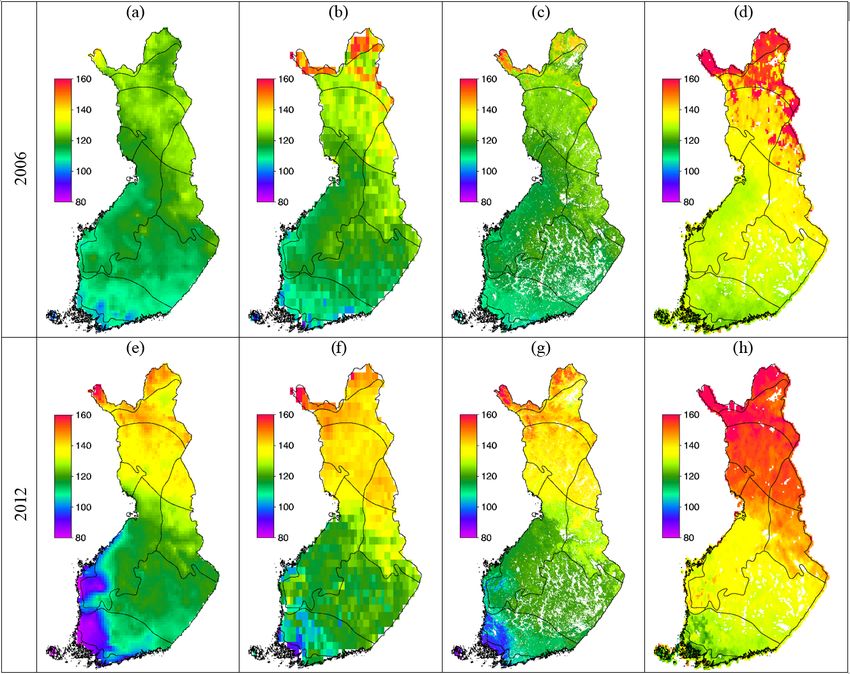
224                                                  T. Manninen et al.: Monitoring changes in forestry and seasonal snow

ical of Arctic and subarctic areas) to coniferous, would de-      ice and land surface components (or ecosystem models) of
crease the albedo of the snow-covered season noticeably.          the climate models have difficulties in correct representation
Previously, it has been shown that the climatic and vegeta-       of the inter-annual variability of the Arctic sea ice cover and
tional zones are equivalent in the boreal forests (Solantie,      terrestrial snow cover. Therefore, observations of snow and
2005). Hence, a significant change in climate would result        its annual cycle are needed to discover the recent trends. Fur-
in a change in vegetational zones.                                thermore, when climate model output is used to drive a land
   Changes in land management may already have a signifi-         ecosystem model to predict the evolution of snow cover, it is
cant effect on surface temperature, equal to that of land cover   necessary to adjust climatic variables with observational data
change (Luyssaert et al., 2014). Changes in forest manage-        e.g. by means of bias-correction methodologies.
ment practices can markedly affect the boreal forest albedo          The EU Life+ MONIMET (http://monimet.fmi.fi, last
through changes in leaf area index (LAI), biomass or canopy       access: 14 January 2019) project aimed at increasing the
density, especially in winter and spring when the forest floor    turnover of climate and other data sources and creating in-
is covered by snow. In Finland, the forests are to a large ex-    dicators of seasonal fluctuations that can be used to assess
tent managed, and the changes in forest structure and stock-      the vulnerability of boreal forest and peatland ecosystems
ing are monitored by the National Forest Inventory (Tomppo        to climate change. The approach was based on a combina-
et al., 2011).                                                    tion of climate data, models, field observations, phenologi-
   In the future, the average temperature in Finland will rise    cal camera network, eddy-covariance measurements and re-
more (Ruosteenoja et al., 2016a) and faster than the global       mote sensing, which together can provide a comprehensive
average (Ruosteenoja et al., 2016b; Parry et al., 2007). Also     view on the changes in the phenology of vegetation, snow
the precipitation is estimated to increase, but in winter more    cover, and ecosystem carbon and heat cycle (Böttcher et al.,
of it will be rain than snow (Jylhä et al., 2012). On aver-       2014, 2016; Linkosalmi et al., 2016; Arslan et al., 2017; Pel-
age, the changes will be larger in winter than in summer          toniemi et al., 2018a; Tanis et al., 2018). Satellite data sets
(Ruosteenoja, 2013; Ruosteenoja et al., 2016b). Warming           processed in the MONIMET project were specifically used
will be fastest in northern Finland (Ruosteenoja, 2013) and       to derive large-scale indicators for the growing season and
very low temperatures seem to appear more rarely. However,        the snowmelt onset and melt-off date.
sub-freezing temperatures will persist in the northern parts         In this work we study whether there were changes of sig-
of the country. It is anticipated that the snow cover period      nificant scale in snowmelt period and winter albedo dur-
will become shorter especially in southern Finland, while in      ing recent decades, 1982–2016, and compare the trends to
northern Finland the snow depth may actually increase due         changes in forest biomass. The surface albedo data record,
to increased snowfall. Generally, the observations indicate a     CLARA-A2 SAL (Anttila et al., 2016a, b; Karlsson et al.,
larger decreasing trend in snow extent during spring than the     2017), was used to study trends in the snowmelt start and
global climate models (Derksen and Brown, 2012; Thack-            end dates, the melting season length and the albedo value
eray et al., 2016). The variation between diverse model re-       preceding the melt onset. We also use the snow-melt-off date
sults is large and can be partly attributed to missing or over-   derived from the EU FP7 CryoLand project Pan-European
simplified process descriptions.                                  Fractional Snow Cover (FSC) time series available for years
   Arctic warming has caused the Arctic sea ice extent to de-     2001–2016 (Metsämäki et al., 2018). The snowmelt end
cline rapidly (Vihma, 2014). There is evidence that such a de-    dates operationally produced at the Finnish Meteorological
cline, together with changed heat and moisture budgets and        Institute (FMI) from weather station observations are used as
increased snow cover in Eurasia, is connected to the change       reference data. In addition, we use the land ecosystem model
towards atmospheric circulation patterns resembling the neg-      JSBACH (Raddatz et al., 2007; Reick et al., 2013) to derive
ative phase of the North Atlantic Oscillation and Arctic Os-      snowmelt onset and end dates for the time range 1981–2011.
cillation, favouring cold winters in Europe and northeastern      The hourly climatic forcing for the land ecosystem model
Eurasia. According to observations, cold, snow-rich winters       was produced with a regional climate model REMO (Jacob
have become more common again in large parts of Europe            and Podzun, 1997; Jacob et al., 2001) that was constrained
since 2005 (e.g. Cohen et al., 2010, 2012; Petoukhov and          with ERA-Interim weather (Dee et al., 2011) and further
Semenov, 2010; Osborn, 2011). Global climate models have          bias corrected (Räisänen and Räty, 2013; Räty et al., 2014)
challenges in representing the recent changes in the Arctic.      with FMI gridded temperature and precipitation data (Aalto
The models may underestimate the observed negative Arctic         et al., 2013) to minimize the climate model inherent biases
Oscillation due to sea ice and snow cover changes (Handorf,       (Böttcher et al., 2016). The changes in the albedo values pre-
2015). The strengthening and westward shift of the Siberian       ceding the melting season are compared with trends in the
high-pressure system is too weak in the models as compared        stem volume in order to evaluate whether the changes in the
to reanalysis data (Dee et al., 2011). The models have prob-      forest explain the changes in albedo. The stem volume values
lems in the gravity wave response and upward vertical prop-       per forest centre area were obtained from the National Forest
agation (Vihma, 2014). They have not reproduced the ob-           Inventory data sets. An albedo model (Manninen and Sten-
served winter cooling over large parts of Eurasia, and the sea    berg, 2009) is used to link stem volumes, LAI and albedo.

Biogeosciences, 16, 223–240, 2019                                                       www.biogeosciences.net/16/223/2019/
T. Manninen et al.: Monitoring changes in forestry and seasonal snow                                                                 225

                                                                         decades. In the regional sampling, the country was divided
                                                                         up into 15 forest centres. One or more regions (forest centres)
                                                                         were inventoried each year, while all regions were invento-
                                                                         ried during the full inventory period (5–7 years). After finish-
                                                                         ing one inventory period, a new inventory period started and
                                                                         regions were inventoried again. More recently, in and since
                                                                         inventory no. 10 the whole area of Finland has been inven-
                                                                         toried within 1 year, but with lesser density. The full sam-
                                                                         pling density was reached within the inventory period, and
                                                                         forest resource estimates were again published. We assigned
                                                                         the forest volume estimates of newer inventories (10 and 11)
                                                                         to the mean years of the inventory periods. The northernmost
                                                                         forest centre, Lapland, further provides the estimates sepa-
                                                                         rately for the northern and southern parts in the most recent
                                                                         forest inventory.
                                                                            The types and fraction of the forest area in each forest cen-
                                                                         tre are shown in Table 2, as well as the average solar-zenith-
                                                                         angle value at melt onset time. The narrow coastal areas of
                                                                         Åland and the Southern and Ostrobothnian coasts were re-
Figure 1. The regions based on the vegetation zones (a) and the re-
                                                                         moved from the analysis due to mixed pixel problems of the
gions of the forest centres (b) of Finland. The Finnish territory (in-
cluding islands) is situated between the latitudes 59.5 and 70.1◦ N      satellite-based albedo product.
and the longitudes 19.1 and 31.6◦ E.
                                                                         2.1.3   Snow cover melt-off data

2     Materials and methods                                              The snow cover melt-off date used operationally at the
                                                                         Finnish Meteorological Institute is defined to be the first day
2.1     Data sets                                                        after the longest period of complete snow cover in a win-
                                                                         ter when open areas have been continuously at least half
2.1.1    Vegetation zones                                                covered by snow from the day of the beginning of perma-
                                                                         nent snow cover (Solantie et al., 1996; Kersalo and Pirinen,
The digital vegetation zone map of Finland was provided by               2009). Complete disappearance of snow cover in open areas
the Finnish Environment Institute (SYKE). The area was re-               is reached typically 10 days later (Solantie et al., 1996). The
duced to 13 main regions (Fig. 1, Table 1) by removing small             snow-melt-off dates were calculated using the in situ snow
islands from the map. Since the surface albedo product used              depth measurements and the results were interpolated in a
in this study has a spatial resolution of only 0.25◦ , the re-           10 km × 10 km grid.
moved smaller islands would cause mixed pixel problems.
Even now the narrow coastal areas (Åland, Ostrobothnian
coast) are prone to extra scatter due to mixed pixels. Hence,            2.1.4   Surface albedo data
they were removed from the final analysis. The vegetation
zones stretch from hemiboreal to northern boreal.                        The data record used in this study (CLARA-A2 SAL) covers
                                                                         the years 1982–2015 and is based on homogenized AVHRR
2.1.2    Forest data                                                     data. It has been developed in the Satellite Application Facil-
                                                                         ity project on Climate Monitoring, CM SAF, which is finan-
The National Forest Inventory of Finland surveys forests                 cially supported by the European Organization for the Ex-
based on a uniform and dense sampling grid and provides                  ploitation of Meteorological Satellites (EUMETSAT). The
unbiased estimates of forest volume and other forest vari-               data record is described in more detail in Anttila et al. (2016a,
ables. The results of the inventories have been estimated for            b, 2018) and Karlsson et al. (2016, 2017). The retrieved
15 forest centres (Fig. 1) in inventory reports (Korhonen et             albedo is defined to the wavelength range 0.25–2.5 µm and
al., 2000a, b, 2001, 2013, 2017; Salminen, 1993; Salminen                the observations are averaged to a 0.25◦ grid, which is also
and Salminen, 1998; Tomppo et al., 1998, 2001, 2003, 2004,               the resolution of the final product. The albedo values are
2005). In this study, we compiled time series of forest volume           given in the range 0 %–100 %. The annual mean surface
and area estimates of forests based on published inventory re-           albedo values preceding the onset of snowmelt were deter-
ports.                                                                   mined for the 13 regions matching the vegetation zones of
   The sampling system of the National Forest Inventory has              Finland and for the 16 forest centre areas of Finland. Also
changed from regional to continuous sampling in the past                 the mean starting and end dates of the snowmelt and the

www.biogeosciences.net/16/223/2019/                                                                Biogeosciences, 16, 223–240, 2019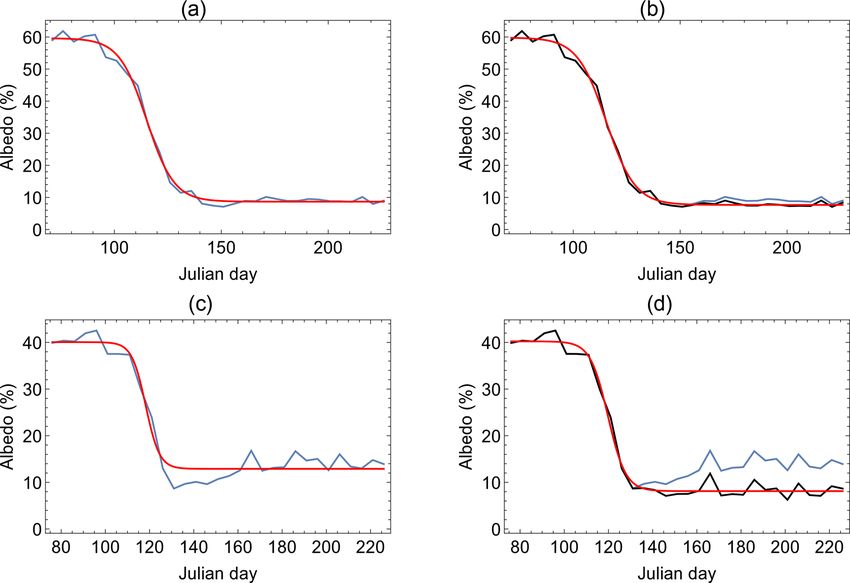
226                                                      T. Manninen et al.: Monitoring changes in forestry and seasonal snow

Table 1. The regions based on the vegetation zones of Finland.

                                 Region     Name                           Type              Number of
                                                                                             SAL pixels
                                 1          Åland                          Hemiboreal                 3
                                 2          Oak zone                       Hemiboreal                19
                                 3          Southwestern Finland           Southern boreal          127
                                 4          Southern Ostrobothnia          Southern boreal           19
                                 5          Lake district                  Southern boreal          224
                                 6          Northern Karelia–Kainuu        Middle boreal            112
                                 7          Ostrobothnia                   Middle boreal            212
                                 8          Southwestern Lapland           Middle boreal             23
                                 9          Kuusamo district               Northern boreal           47
                                 10         North Ostrobothnia             Northern boreal          130
                                 11         Northwestern Fjeld Lapland     Northern boreal           20
                                 12         Forest Lapland                 Northern boreal           86
                                 13         Northern Fjeld Lapland         Northern boreal           30

Table 2. The regions based on the forest centres of Finland.

         Region     Name                                  Mean solar     Mean fraction   Type                         Number
                                                         zenith angle      of forested                                of SAL
                                                           at onset of            area                                 pixels
                                                            snowmelt              (%)
         1          Åland                                        64.9◦              59   Hemiboreal                       40
         2          Southern and Ostrobothnian coast             63.5◦              62   Hemiboreal–southern boreal       63
         3          Southwestern Finland                         63.7◦              62   Hemiboreal–southern boreal       76
         4          Häme–Uusimaa                                 62.4◦              67   Southern boreal                  52
         5          Southeastern Finland                         63.3◦              74   Southern boreal                  50
         6          Pirkanmaa                                    62.9◦              75   Southern boreal                  48
         7          Ostrobothnia                                 64.6◦              70   Middle boreal                    57
         8          South Ostrobothnia                           61.4◦              71   Middle boreal                    71
         9          Central Finland                              61.3◦              85   Middle boreal                    64
         10         Etelä-Savo                                   62.2◦              85   Southern boreal                  60
         11         Pohjois-Savo                                 60.4◦              81   Middle boreal                    66
         12         North Karelia                                60.2◦              84   Middle boreal                    68
         13         North Ostrobothnia                           60.3◦              77   Middle–northern boreal          145
         14         Kainuu                                       59.5◦              87   Middle boreal                    77
         15         Southern Lapland                             59.0◦              81   Northern boreal                 220
         16         Northern Lapland                             57.8◦              51   Northern boreal                 103

length of the melting season were calculated for those re-               but is also able to capture the under-canopy snow. This type
gions (Sect. 2.2.1).                                                     of snow product featuring snow on ground, not just view-
                                                                         able snow, shows high FSC if the forest floor (and under-
2.1.5   Fractional snow cover data                                       subcanopy low vegetation) is snow covered, even though
                                                                         from the satellite sensor’s point of view the forest looks
At-pixel fractional snow cover (% of ground area covered by              darker in terms of albedo. The gained accuracy (using in situ
snow) is extracted from the pre-Copernicus CryoLand snow                 FSC observations at Finnish snow transects as reference) is
mapping service (Nagler et al., 2015), which provides Pan-               15 %–20 %.
European FSC maps starting from 2001 at 500 m (0.05◦ ) spa-
tial resolution. The method applied in the FSC retrieval is              2.1.6    MODIS data
SCAmod (Metsämäki et al., 2005, 2012), complemented by
some additional NDSI (normalized difference snow index)                  Daily composites of Moderate Resolution Imaging Spectro-
rules for detecting the snow-free areas (Metsämäki et al.,               radiometer (MODIS) data were used for the determination of
2018). SCAmod detects FSC not only for non-forested areas,               the start of growth of deciduous canopy (Sect. 2.2.4) during

Biogeosciences, 16, 223–240, 2019                                                               www.biogeosciences.net/16/223/2019/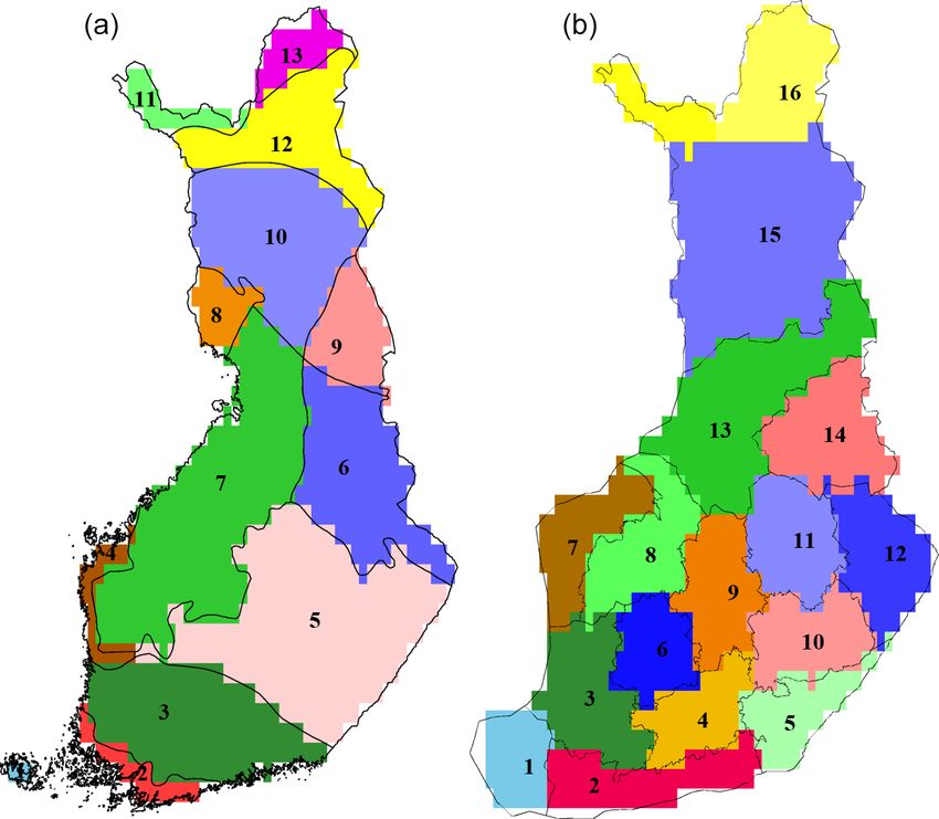
T. Manninen et al.: Monitoring changes in forestry and seasonal snow                                                             227

the period 2001–2016. The Terra MODIS level-1B data were            fitting in Fig. 2). The updated albedo curve was then used as
retrieved from the National Aeronautics and Space Adminis-          the basis of a new sigmoid fit with the maximum number of
tration (NASA)’s Level 1 product and Atmosphere Archive             iterations being five. If the value of the coefficient of deter-
and Distribution System (LAADS) and, from 2010 onwards,             mination R 2 was smaller for the second sigmoid fit than for
from the receiving station of the Finnish Meteorological In-        the first fit and R 2 was smaller than 0.99 for the first fit, the
stitute at Sodankylä. The data were processed to top-of-            latter sigmoid fit was carried out anew with the maximum
atmosphere (TOA) reflectances and projected into a geo-             number of iterations being now increased to 15. Finally, the
graphic latitude and longitude grid. The normalized differ-         sigmoid of the two rounds that had on average the smallest
ence water index (NDWI) was calculated from near-infrared           fit residuals was chosen.
(841–876 nm) and mid-infrared (1628–1652 nm) TOA re-                    In some cases, the snowmelt onset could not be deter-
flectances (Gao, 1996). Further details of the preprocessing        mined, because it had started already before the first cloud-
are given in Böttcher et al. (2016).                                free albedo pentad was available for the pixel and year in
                                                                    question. For the regional mean values of the melt onset and
2.2     Melting season start and end determination                  end dates and albedo at the melt onset date, only the pixels
                                                                    for which the melt onset date was available were included in
2.2.1    Start and end date of snowmelt season from                 the analysis.
         surface albedo data
                                                                    2.2.2   Start and end date of snowmelt season from
Previously, the end of the melting season of seasonal snow                  ecosystem models
has been successfully estimated using the standard devia-
tion of the weekly means of albedo data (Rinne et al., 2009).       The JSBACH land surface model (Raddatz et al., 2007; Reick
Now, the CLARA-A2 SAL pentad mean albedo values were                et al., 2013) resolves land surface physical and biogeochem-
studied by fitting sigmoids matching the melting season, us-        ical processes involved in surface energy balance as well as
ing nonlinear regression similar to the method by Böttcher          water and carbon balances within soil and vegetation. In ad-
et al. (2014). For each pixel and year, the pentads from the        dition to its principal use to serve as a land surface boundary
end of January until the end of August were used. The date          for the Max Planck Institute for Meteorology Earth System
of snowmelt onset was taken to be the date at which the sig-        Model (MPI–ESM) (Stevens et al., 2013), JSBACH can be
moid reached 99 % of its variation range. Similarly, the end        driven with prescribed weather data. In this work, JSBACH
of the snowmelt season was defined to be the day in which           was driven using the bias-corrected hourly REMO data for
the sigmoid reached 1 % of its variation range. The length of       the years 1980–2011 with a spin-up period of 30 years before
the melting season was then the difference between these two        the forward run to equilibrate soil water and soil tempera-
dates. The albedo value corresponding to the onset of melt-         ture. The spatial domain of JSBACH is also Fennoscandia at
ing was used as the representative albedo value preceding the       a resolution of 0.167◦ , but in the present study only Finnish
melting season (Anttila et al., 2018).                              territory is investigated.
   At first, a rough sigmoid fitting was carried out iteratively,      The JSBACH set-up used requires seven mutually consis-
with the maximum number of iterations being five. The rea-          tent meteorological drivers: 2 m air temperature (Tair ) and
son for iteration is that the nonlinear fit outcome depends on      specific humidity, 10 m wind velocity, short-wave and long-
the choice of initial parameter values of the nonlinear func-       wave radiation, potential short-wave radiation and precipita-
tion to be fitted. After that, the albedo values lower than the     tion (Pr ) prescribed in hourly time resolution. For providing
mid-sigmoid values were removed from the period preced-             these drivers we used the regional climate model REMO (Ja-
ing the melting season as temporary melt events. Similarly,         cob and Podzun, 2007; Jacob et al., 2001) with an implemen-
possible albedo values higher than mid-sigmoid values were          tation of surface properties by Gao et al. (2015). The mod-
removed from the period succeeding the melting season as            elling domain for REMO was Fennoscandia, with a grid reso-
temporary snowfalls or cloud masking errors of the albedo           lution of 0.167◦ , corresponding approximately to 18 km. Lat-
product. Then the sigmoid was fitted anew, using again a            eral boundary data were taken from ERA-Interim, a global
maximum of five iterations. In some areas, right after the end      atmospheric reanalysis produced by the European Centre for
of the snowmelt, new growth of vegetation started to increase       Medium-Range Weather Forecasts (ECMWF) (Dee et al.,
the albedo level so soon that it affected the sigmoid fitting.      2011). The forward run covered the period from 1979 to 2011
Therefore, the minimum albedo value starting from the mid-          and it was preceded by a 10-year spin-up to equilibrate soil
sigmoid was sought. A second order polynomial was fitted            moisture and temperature.
to the part of the albedo curve starting from that point. This         Model-specific biases are inherent for regional climate
regression polynomial was used to remove the growing sea-           models (Christensen et al., 2008; Teutschbein and Siebert,
son increase in the albedo but leave the pointwise variation        2012) and it is known that REMO exhibits too-cold winter
of that part of the original curve (i.e. the blue curve of origi-   temperatures in an Eastern European area that covers most
nal data is replaced with the black curve in further nonlinear      of Finland (Pietikäinen et al., 2012; Gao et al., 2015). The

www.biogeosciences.net/16/223/2019/                                                            Biogeosciences, 16, 223–240, 2019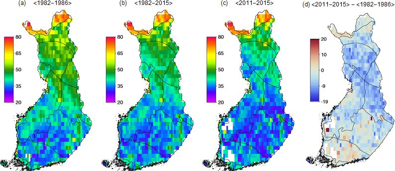
228                                                                T. Manninen et al.: Monitoring changes in forestry and seasonal snow

Figure 2. Examples of sigmoid fitting. The original data points are shown in blue; the fit in red; and the data points, from which the vegetation
greening effect has been removed, in black. (a) Initial fit of the easy case, (b) final fit of the easy case, (c) initial fit of a case with strong
influence of vegetation greening on albedo and (d) final fit of the case with strong influence of vegetation greening on albedo.

modelled summer and autumn temperatures tend to exceed                          canopy. In addition to the snowfall fraction the fate of the
observations. Moreover, REMO overestimates precipitation                        canopy reservoir is constrained by sublimation and melting
in northern Europe throughout the year. To account for the                      that is temperature regulated and due to wind-blow (Roesch
biases, we adjusted air temperature and precipitation against                   et al., 2001). Furthermore, the accumulation of snow is lim-
gridded homogenized weather data for 1980–2011 provided                         ited by LAI. At the ground the snow budget composes of the
by the Finnish Meteorological Institute (Aalto et al., 2013)                    excess snowfall fraction after canopy interception, sublima-
using a quantile–quantile type bias-correction algorithm for                    tion and melting.
daily mean temperature (Räisänen and Räty, 2013), while                            The snow depth was used as an indicator of the melt-
daily cumulative precipitation was adjusted using parametric                    ing season start and end. During early spring the changes
quantile mapping (Räty et al., 2014). Finally, the daily cor-                   in model albedo are very strongly dominated by changes in
rections were applied to the hourly modelled air temperature                    snow cover, since the changes in the leaf area of the conifer-
and precipitation values.                                                       ous forest are minor and the bud burst of broadleaved forest
   In JSBACH surface grid cells are divided into fractions                      occurs later in spring. The modelled melting season timing
of four most prevalent plant functional types (PFT) that are                    and duration were studied by fitting a sigmoid to each grid
characterized with properties such as maximum leaf area,                        cell of the yearly springtime snow depth data. The fit was
phenology type, growth rate, shedding rate and photosynthe-                     done in two phases: the first sigmoid was fitted between days
sis parameters. In addition to PFT fractions, each grid cell is                 of year 30 and 200 to include days of yearly maximum and
characterized with a maximum fraction of the land area that                     minimum snow cover. As modelled snow cover did not typ-
can support plant growth.                                                       ically show a plateau before the start of the melt period, but
   Snowfall fraction of the total precipitation is given as fol-                tended to increase monotonously until the start of the melt-
lows:                                                                           ing, values lower than the first fit were rejected from the part
                                                                                of the time series prior to the point where the sigmoid reaches
                                            Tair > 3.3 ◦ C
           (
               0,
Pr _sn =       Pr · (3.3◦ − Tair )/4.4◦ ,   −1.1 ◦ C < Tair < 3.3 ◦ C .   (1)   its half of the range value. If fewer than 15 data points were
               Pr ,                         Tair < −1.1 ◦ C                     left after the rejection, the grid cell in that year was rejected.
                                                                                Otherwise the sigmoid was fitted to the remaining data se-
Pr_sn is further distributed to surface and canopy reservoirs                   ries. After the second fit a sanity check was made to reject
with the constant fraction of 0.25 to be intercepted by the

Biogeosciences, 16, 223–240, 2019                                                                      www.biogeosciences.net/16/223/2019/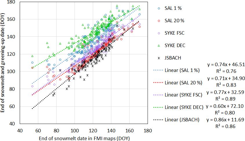
T. Manninen et al.: Monitoring changes in forestry and seasonal snow 229
the fittings implying either a too-small or too-large differ-
ence between the sigmoid parameter values representing the
snow cover levels before and after the melting. Because the
snowmelt starts rather gradually and ends abruptly in the
modelled snow depth data, asymmetric criteria of 98 % and
8 % of the sigmoid variation range were used for the start
and end dates of the melting period, respectively. Finally, for
each vegetation zone yearly regional means of start and end
dates were calculated.
2.2.3 Snow-melt-off date from fractional snow cover
data
The detection of the snow-melt-off date from the FSC map
time series provides for each pixel the first day with snow- Figure 3. Optimal values of k as a function of the fraction of the
free terrain, but ignores short (a few days) intervening snow- forested area in the forest centre area (f ). The brown point is not
free periods within a long snow season (Metsämäki et al., included in the regression k = 0.11 + 1347.44 exp(−11f ), because
2018). The melt-off date from the FSC time series is identi- it represents an area dominated by deciduous species (mountain
fied as the beginning of a snow-free period (FSC = 0 %) after birch).
a period of snow observations (FSC > 0 %). A pixel is as-
signed the status “melted” after a period of at least six subse-
quent snow-free days is found (however with possible inter- of the sun zenith angle of the forest centres at the start day of
vening cloudy observations) if the number of the snow-free snowmelt was used in the calculations (Table 2). The snow
days represents 80 % of all cloud-free observations after the cover of the forest floor is described using its albedo. The for-
first day of the snow-free period of interest. The first day of est inventory does not contain LAI information and a strong
this period is accepted as a candidate for the melt-off date. relationship between the stem volume and LAI cannot be ex-
After the candidate day, a new snow period is allowed if at pected at a high spatial resolution. Yet, in larger areas one
least three subsequent snow-covered days are observed. Then could assume that the LAI of a forest is statistically related
a new search for the melt-off date is launched the same way to the stem volume per area V according to LAI = kV 2/3 .
as before. When comparing the albedo simulations to the satellite mea-
surements in a larger area, one has to take into account also
2.2.4 Start of the growing season of deciduous canopy the fraction of the forested area. The albedo of the forest cen-
from MODIS data tre areas was simulated for the years matching the National
Forest Inventory during 1963–2011 varying the coefficient
The start of the growing season of deciduous vegetation k in the range 0.1–1.5. The optimal value of k was defined
in Finland, usually referred to as greening up, was deter- to be the value corresponding to smallest difference between
mined from NDWI using the method described in Böttcher the simulated and satellite-based albedo values. A relatively
et al. (2016). The NDWI was utilized because the detection strong relationship between the optimal value of k and the
of the greening up in boreal areas from the normalized dif- fraction of the forest area in the boreal forest zone was found
ference vegetation index (NDVI) can be affected by melting (Fig. 3). The area left outside the regression (Northern La-
of snow, whereas the NDWI allows a differentiation between pland) is dominated by deciduous species (mountain birch);
snowmelt and greening up (Delbart et al., 2006). The start hence its LAI value in winter is not related to the stem vol-
of the growing season showed good correspondence with the ume similarly as for the coniferous species.
date of birch bud break (RMSE of 1 week) at Finnish phe-
nological sites when the corresponding MODIS pixels are
dominated by deciduous forest. The data set for the period 3 Results
2001–2016 has a spatial resolution of 0.5 × 0.5◦ .
3.1 Seasonal snowmelt timing
2.2.5 Albedo model calculations
3.1.1 Snowmelt onset
The effect of snow cover on surface albedo of coniferous
forests can be estimated using an albedo model based on The onset of melting was determined using the sigmoids de-
the photon recollision probability (Manninen and Stenberg, termined both from the satellite-based albedo data, CLARA-
2009). The forest parameters required are LAI, the clumping A2 SAL pentads, and the daily JSBACH model calculations
factor and the single-scattering albedo of needles. In addi- of the snow depth. The comparison of these melting season
tion, the sun-zenith-angle value is needed. The average value start dates is shown in Fig. 4. The overall agreement is good,
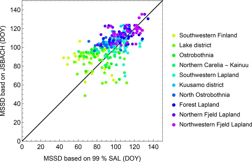
www.biogeosciences.net/16/223/2019/ Biogeosciences, 16, 223–240, 2019230 T. Manninen et al.: Monitoring changes in forestry and seasonal snow
and some of the scatter can be attributed to using a different
variable for the data (albedo) and the model (snow depth).
For the model calculations, the snow depth was used as the
indicator of the snowmelt onset rather than the albedo, be-
cause the snow depth is more related to the snow accumula-
tion throughout the seasonal cold period, whereas the albedo
is sensitive to the prevailing weather conditions just before
the melt onset. The snow depth describes the whole snow-
pack, whereas the albedo describes only the topmost layer of
it. The surface albedo product showed a negative trend (about
half a day per year) in two areas: Northern Karelia–Kainuu
and Southwestern Lapland (Table 3, Fig. 5). For the other
areas, the coefficient of determination for a linear trend of
5-year average values was smaller than 0.5. The annual vari-
ation of the melt onset date is so large (the standard deviation Figure 4. The melt onset day of the snow cover in Finland during
being on average 12 days for the time range 1982–2015) that 1982–2011 based on the CLARA-A2 SAL product and JSBACH
it easily masks a long-term trend. This was even more evident model snow depth.
in the land ecosystem model calculation results, for which a
low frequency variation dominated the time window so that
based melt-off date refers to the end of the permanent snow
no region showed a marked trend even in the 5-year mov-
cover when half of open areas still have snow (Fig. 6). The
ing average curve. In particular, variable melt onset timing
1 % threshold for the albedo produced a clearly later end of
is in the coastal regions (Southwestern Finland and South-
the melt date than the in situ-based snow-melt-off date and
ern Ostrobothnia) and in the Lake district. For those regions,
model results. This is understandable, because the FMI op-
the standard deviation values of the melt onset date are 14.3,
erational melt-off date does not correspond to a completely
14.7 and 14.6, respectively. For the Northern Fjeld Lapland,
snow-free case and the albedo value is very sensitive to even
the vicinity of the Barents Sea also causes a higher standard
small amounts of snow. The day in which the albedo-based
deviation (13.4) of the melt onset date. A large part of Fin-
sigmoid reached 20 % of its variation range matched the of-
land is coastal, and consequently the sea ice extent of the
ficial end date of snowmelt well and the 15 % value matched
Baltic Sea has a strong effect on the weather and climate, not
the FSC-based melt-off date well. The difference between
only changes in air temperature or precipitation preceding the
dates corresponding to the 20 % and 1 % threshold values of
melt onset, which are the dominating drivers in some regions
the albedo-based sigmoids is of the order of 13 days, which is
of the Northern Hemisphere (Anttila et al., 2018). When us-
in line with the 10-day difference, during which half of snow-
ing 10-year moving averages for the trend analysis based on
free open areas become completely snow-free (Solantie et
the albedo data, a negative trend (R 2 > 0.5) of the melt onset
al., 1996). Results from JSBACH coincide well with the op-
date was detected in Northern Karelia–Kainuu, Southwest-
erationally observed end of permanent snow cover. Probably
ern Lapland, Ostrobothnia, Kuusamo district and Lake dis-
the snow-off bias inherited from the climate model surface
trict. Although the time series of 34 years is not really long
parametrizations explain why the zero value of snow depth
enough for using 10-year averages, the results, however, con-
of JSBACH matches the time when half of open areas are
firm the intuitive impression that the snowmelt starts earlier
snow-free. It has been shown that, for example in ECHAM5,
than it used to do in the past, as the two distinct areal trends
the snowmelt occurs at too-low temperatures (Räisänen et al.,
showed.
2014). Consequently, too much of the surface net radiation is
consumed in melting snow and too little in heating the air.
3.1.2 End of snowmelt
No systematic trend was observed for the end of snowmelt
date for moving 5-year averages of the albedo or the land
The end of snowmelt was determined using the albedo data,
ecosystem model data. It seems that the onset of snowmelt
the snow depth value of the land ecosystem model and the
depends more clearly on the climate and the end of snowmelt
snow-melt-off date derived from the satellite-based fractional
is more sensitive to the prevailing weather conditions at that
snow cover estimate for each area of the vegetation zone
time.
map. The results were compared with the FMI snowmelt
The areal advance of spring is demonstrated by the FMI
maps provided operationally by the climate service of FMI
operational melt-off map, the surface albedo 20 % threshold
(Solantie et al., 1996; Fig. 6). The overall agreement is
map, the FSC melt-off map and the greening-up map in years
good for the melt-off date derived from MODIS-based FSC
2006 and 2012 (Fig. 7). The general agreement is good, and
and the FMI operational melt-off date derived using in situ
the overall zones of equal timing are obvious.
data taking into account that the satellite-based melt-off date
refers to a completely snow-free case, whereas the in situ-
Biogeosciences, 16, 223–240, 2019 www.biogeosciences.net/16/223/2019/T. Manninen et al.: Monitoring changes in forestry and seasonal snow 231
Table 3. The observed trends of the melt onset and melting season length during 1982–2015 according to the CLARA-A2 SAL data of the
regions based on the vegetation zones (Table 1). Values for the slope and the coefficient of determination are shown both for annual data
and for moving averages of 5 years. The cases for which the moving average of 5 years shows a significant coefficient of determination are
indicated with bold fonts.
Region Melt onset Melting season length
Annual value Moving average of 5 years Annual value Moving average of 5 years
Slope R2 Slope R2 Slope R2 Slope R2
(days per (days per (days per (days per
decade) decade) decade) decade)
Northern Fjeld Lapland 2.1 0.024 1.3 0.041 −6.3 0.097 −6.2 0.22
Forest Lapland −0.03 0.0000067 −0.7 0.02 −1.5 0.0094 −1.4 0.033
Northwestern Fjeld Lapland 1.0 0.0076 0.6 0.014 −2.4 0.023 −3.1 0.13
North Ostrobothnia −2.6 0.071 −3.3 0.33 3.9 0.12 4.3 0.44
Kuusamo district −2.1 0.047 −3.3 0.34 3.0 0.052 4.7 0.35
Southwestern Lapland −4.7 0.17 −5.0 0.78 6.6 0.16 6.8 0.67
Ostrobothnia −3.5 0.083 −4.3 0.41 2.0 0.022 3.3 0.18
Northern Karelia–Kainuu −5.3 0.19 −6.3 0.81 5.8 0.12 7.1 0.68
Lake district −2.4 0.027 −3.7 0.23 −0.3 0.00038 1.7 0.028
Southwestern Finland 0.8 0.0027 −1.5 0.051 −6.4 0.098 −4.0 0.072
Figure 5. Trends of the melt onset day of the snow cover in Northern Karelia–Kainuu and Southwestern Lapland during 1982–2015 based
on the CLARA-A2 SAL product. The solid curves represent the 5-year moving averages and the dotted curves the annual values.
3.1.3 Length of the melting season of snow trict, Southwestern Lapland and North Ostrobothnia and de-
creased in Northern Fjeld Lapland.
The length of the melting season was determined as the dif-
ference between the dates corresponding to the end of the 3.2 Start of the growing season
snowmelt and the onset of the snowmelt. The 99 % and
1 % threshold values were used for the albedo sigmoids. A The start of the growing season of deciduous vegetation
clear trend of increasing melting period length was observed based on MODIS NDWI values turned out to almost coin-
for moving 5-year averages of the areas Northern Karelia– cide with the timing of the 1 % threshold value of the surface
Kainuu and Southwestern Lapland, where the snowmelt albedo, being only slightly later (Fig. 6). This is probably due
starts earlier than before (Table 3, Fig. 8). For the length of to the large fraction of deciduous species being in open areas
the melting season, the standard deviation during 1982–2015 and on the forest floor, where the growing starts only after
was on average, naturally, even larger than for the melt onset the soil has become completely snow-free and where even
date, with the value being as high as 16 days. The largest val- small amounts of remaining snow have a large effect on the
ues occurred again in Southwestern Finland (20.3), South- albedo. The difference between the date when the SAL value
ern Ostrobothnia (17.5), Lake district (17.1) and Northern reached 1 % of its dynamic range during the melting season
Fjeld Lapland (20.0). When using 10-year moving averages and the date of the greening up varied in the vegetation zones
in the trend analysis, the result was that the melting season on average between 5 and 13 days during the 16 years of
length increased in Northern Karelia–Kainuu, Kuusamo dis- comparison. The largest difference took place on the coast
www.biogeosciences.net/16/223/2019/ Biogeosciences, 16, 223–240, 2019232 T. Manninen et al.: Monitoring changes in forestry and seasonal snow Figure 6. Comparison of diverse estimates of the melt-off day of snow cover. The FMI snow maps of end of permanent snow cover are based on in situ snow depth measurements. The satellite-based melt-off date estimates are derived using the surface albedo product CLARA-A2 SAL (Anttila et al., 2016a; Karlsson et al., 2017) and the FSC snow product calculated from MODIS images (Metsämäki et al., 2018). The JSBACH model estimate of end of snowmelt is also shown. For comparison the greening-up date of deciduous vegetation (SYKE DEC; Böttcher et al., 2016) is also presented. Figure 7. The progress of spring in 2006 and 2012 starting from (a, e) the melt-off day of the permanent snow cover in Finland based on in situ snow depth measurements (Solantie et al., 1996; Kersalo and Pirinen, 2009), (b, f) the surface albedo reaching the 20 % threshold value of its dynamic range during the melting season (Anttila et al., 2016a; Karlsson et al., 2017), (c, g) the complete disappearance of the snow cover based on the FSC product (Metsämäki et al., 2018) and (d, h) the greening-up day based on MODIS NDWI (Böttcher et al., 2016). Biogeosciences, 16, 223–240, 2019 www.biogeosciences.net/16/223/2019/
T. Manninen et al.: Monitoring changes in forestry and seasonal snow 233
Figure 8. Trends of the melting season length of the snow cover in Northern Karelia–Kainuu and Southwestern Lapland during 1982–2015
based on the CLARA-A2 SAL product. The solid curves represent the 5-year moving averages and the dotted curves the annual values.
and the shortest in mountain areas, where greening of moun- 4 Discussion
tain birch can occur even before the snowmelt (Shutova et
al., 2006; Peltoniemi et al., 2018b). In addition, trees in the Surface albedo is determined by the quantity and type of land
northern boreal region have a lower temperature requirement vegetation, the seasonal cycle of leaf development and the
for bud burst than in the south, and the day length is already existence of snow cover. The snow conditions also depend
longer in the north at the time of bud burst. Therefore, the in- on the vegetation cover. Seasonal dynamics of snow and veg-
tensity of the response to temperature increases from south to etation are driven by temperature and precipitation. The air
north and the observed trend towards earlier bud burst were temperatures in the Arctic and boreal regions have increased
stronger in the northern boreal zone compared to the southern and the Arctic sea ice extent has reduced, and their influ-
boreal zone for the period 1997–2006 (Pudas et al., 2008). ence can be seen in the Finnish temperature and precipitation
records. The trends are not self-evident, although as a whole
3.3 Albedo before onset of snowmelt
the Arctic and boreal region is changing towards a warmer
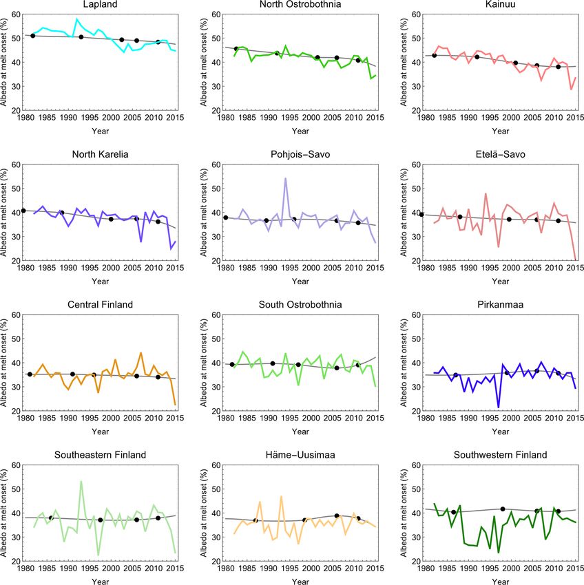
The surface albedo at the melt onset shows a decreasing trend climate. The large variation in the climate can be seen in
in several northern regions based on the vegetation zones (Ta- both observed and modelled snowmelt onset. The observed
ble 4, Fig. 9). This can be explained by the increase in the trends are clearly negative only in Northern Karelia–Kainuu
stem volume, as the albedo model results agree with the ob- and Southwestern Lapland. The year-to-year variation in the
served albedo trends of the forest-centre-based regions (Ta- modelled snowmelt onset is not as large as in the observed
ble 5, Fig. 10). Data showed meaningful trends (R 2 > 0.5) snowmelt onset data, but the multi-year variation is similar,
for 5-year average albedo values only, when the fraction of with the model acting as a smoother of observations. In many
the forested area exceeded 0.7 and the stem volume was cases, both positive and negative tendencies appear during
smaller than 75 m3 ha−1 . For those areas (Southern Lapland, the study period, most significantly around year 2000, when
Kainuu, Northern Ostrobothnia, Lapland and North Karelia), the snowmelt showed a transition from earlier onset to later
the albedo trend is negative. It is well known that the win- onset in Southwestern Finland, Lake district and Ostroboth-
tertime albedo depends strongly on the LAI (and thus stem nia. Also in a previous analysis using a 35-year data set from
volume of a larger area) when the LAI is relatively small the passive microwave radiometer snow clearance data set,
(Manninen and Stenberg, 2009). For larger LAI values, the Metsämäki et al. (2018) concluded that the snow melt-off
albedo more or less saturates, and a further increase in LAI at northern latitudes in Europe has advanced 3–5 days per
does not show up markedly. As expected, no clear albedo decade in boreal forests and tundra. The MODIS FSC-based
trend after the snowmelt was observed. The reason is that snow-melt-off maps of this study gave a similar signal.
the difference between the canopy and forest floor vegetation The trends of the end of the snowmelt are insignificant ev-
albedo is small, whereas the snow and canopy albedo values erywhere. However, combined with the negative snowmelt
differ markedly. Hence, the accumulating stem volume in the onset trend in Northern Karelia–Kainuu and Southwest-
northern part of Finland causes darkening of the winter- and ern Lapland, we obtain an increase in the length of the
springtime albedo, but does not have a significant effect on snowmelt period in those regions. Generally, in northern lati-
the albedo value right after the snowmelt. tudes, many studies have shown persistent negative trends in
snowmelt onset and positive trends in early spring vegetation
activity (Myneni et al., 1997; Pulliainen et al., 2017). A re-
cent study indicated an increase in the length of the snowmelt
period (Contosta, 2017), which could have both negative and
positive impacts for soil water availability, nitrogen cycling,
www.biogeosciences.net/16/223/2019/ Biogeosciences, 16, 223–240, 2019234 T. Manninen et al.: Monitoring changes in forestry and seasonal snow
Table 4. The observed albedo trends of regions based on the vegetation zones. Values for the slope and the coefficient of determination are
shown both for annual data and moving averages of 5 years. The cases for which the moving average of 5 years shows a significant coefficient
of determination are indicated with bold fonts.
Region Annual value Moving average of 5 years
Slope (albedo R2 Slope (albedo R2
in % units per in % units per
decade) decade)
Northern Fjeld Lapland −1.6 0.18 −1.8 0.36
Forest Lapland −2.3 0.52 −2.5 0.69
Northwestern Fjeld Lapland 0.3 0.01 −0.2 0.01
North Ostrobothnia −3.4 0.72 −3.6 0.83
Kuusamo district −3.1 0.66 −3.1 0.82
Southwestern Lapland −3.3 0.61 −3.3 0.75
Ostrobothnia −1.4 0.23 −0.8 0.47
Northern Karelia–Kainuu −3.0 0.58 −2.6 0.84
Lake district −0.3 0.006 0.6 0.15
Southwestern Finland 0.2 0.004 0.5 0.06
Figure 9. The surface albedo (%) at the time of the melt onset in Finland. The average value during 1982–1986 (a), during 1982–2015 (b)
and during 2011–2015 (c). The difference between the last and first 5 years’ average value is shown as well (d). The white pixels on land
represent cases when the melting has already started before the albedo could be retrieved, i.e. when the sun zenith angle was larger than 70◦ .
and ecosystem carbon and energy balance and thus induce influencing growth of the trees (Sutinen et al., 2014). Hentto-
complex perturbation of land-surface–climate feedbacks. nen et al. (2017) studied forest growth changes in Finland in
Snow has a very complex role in the forest ecosystems, 1971–2010 and concluded that 37 % of the observed growth
and many of the snow-related effects could be revealed and increase was associated with environmental factors, which
many analyses could be deepened by including albedo and are probably related to the climate. Further research is re-
snow cover in the analyses. The snow cover directly affects quired about the effects of climate factors on growth and par-
the greatest soil frost depth in winter. Hence, changes in snow ticularly about the effects of insulating snow cover and soil
cover are expected to affect also the amount of wind throw. temperature.
In particular, late autumn, winter and early spring storms will The timber resources in Finnish forests have grown since
be more dangerous for the canopy if the soil is not frozen as the 1950s more than has been removed by logging (National
it used to be in the past (Peltola et al., 1999). The trafficabil- Forest Inventory, 2013). In northern Finland the share of stout
ity of the forested terrain may reduce with earlier snowmelt timber has traditionally been high, so the increase comes
(Kellomäki et al., 2010). In addition, frost affects the roots mainly from small-diameter timber. While carbon storage
of the trees via the soil frost, rendering it as a potential factor in forests has increased, Finland has darkened, which shows
Biogeosciences, 16, 223–240, 2019 www.biogeosciences.net/16/223/2019/T. Manninen et al.: Monitoring changes in forestry and seasonal snow 235
Figure 10. Comparison of observed albedo variation (colour solid curves) of the forest centre areas (Fig. 1, Table 2) during 1982–2015
and corresponding albedo model results based on stem volume measurements (points). The interpolation curves (grey solid curves) of the
modelled annual values are shown as well. The colours match those of the map in Fig. 1b, except for Lapland, which is treated as one area
(15 and 16).
in the negative trend of albedo preceding the snowmelt sea- to grow more densely and become stouter (Pihlainen et al.,
son. The effect of canopy on snow-covered terrain albedo 2014; Baul et al., 2017a, b; Pingoud et al., 2018) suggests
is largest for small LAI values (Manninen and Jääskeläinen, a possibility to combat climate change in regions of already
2018); hence it is understandable that the marked decreas- medium-size canopy without the negative albedo feedback.
ing trend of albedo before the snowmelt season is observed
in northern Finland. In southern Finland, the share of stout
timber has more than quadrupled since the 1950s, yet no 5 Conclusions
trend in pre-melt albedo during 1982–2016 is observed there.
The surface albedo proved to be a suitable indicator of the
Hence, the idea to increase carbon sinks in forests by increas-
snowmelt onset and end of the melting season. Overall agree-
ing the timber resources of existing forests by causing trees
ment was found with corresponding dates determined using
www.biogeosciences.net/16/223/2019/ Biogeosciences, 16, 223–240, 2019236 T. Manninen et al.: Monitoring changes in forestry and seasonal snow
Table 5. The observed albedo trends of the regions based on the forest centres. Values for the slope and the coefficient of determination are
shown both for annual data and moving averages of 5 years. The region Lapland is divided into northern and southern parts as shown in
Fig. 1. The cases for which the moving average of 5 years shows a significant coefficient of determination are indicated with bold fonts.
Region Annual value Moving average of 5 years
Slope (albedo R2 Slope (albedo R2
in % units per in % units per
decade) decade)
Lapland −2.7 0.60 −3.0 0.72
Northern Lapland −1.2 0.18 −1.5 0.40
Southern Lapland −3.3 0.70 −3.4 0.82
North Ostrobothnia −2.1 0.48 −1.7 0.75
Central Finland −0.05 0.0001 0.9 0.19
Etelä-Savo −0.5 0.01 0.4 0.06
Pirkanmaa 0.6 0.02 1.3 0.30
Southwestern Finland 0.5 0.007 1.3 0.11
Southeastern Finland −0.2 0.002 0.6 0.08
Häme–Uusimaa 0.4 0.009 0.3 0.05
Kainuu −3.0 0.58 −2.8 0.81
South Ostrobothnia −0.5 0.02 0.03 0.0003
Pohjois-Savo −1.1 0.07 −0.6 0.11
North Karelia −1.9 0.24 −1.3 0.53
the JSBACH land ecosystem model snow depth data. The op- 5137E8E5FEF904478BBC386333FD8EB0.ku_2 (last access:
erationally provided end of the permanent snow cover date 14 January 2019). The data on the start of the growing sea-
based on in situ data corresponded to about the day when the son (greening up of deciduous vegetation) for the period
surface albedo value reached the lower 20 % of its dynamic 2001–2016 can be viewed online in a web map application
range during the melting season. The end of the snowmelt (http://syke.maps.arcgis.com, last access: 14 January 2019)
and are available for download at the open-data service of
determined using the satellite-based fractional snow cover
SYKE (http://www.syke.fi/en-US/Open_information/Spatial_
data and the JSBACH land ecosystem model snow depth data datasets\T1\textbackslash#P, last access: 14 January 2019).
also agreed well with the corresponding operationally pro- The original FSC data are available from the CryoLand portal
duced date. The day when the surface albedo has decreased (http://neso1.cryoland.enveo.at/cryoclient/, last access: 14 Jan-
to the lower 1 % of its dynamic range is well in line with uary 2019). Forest inventory data are not publicly available, but
the day corresponding to completely snow-free open areas. aggregated values are (http://kartta.luke.fi/index-en.html, last
In addition, the greening-up date followed on average 5–13 access: 14 January 2019).
days later.
According to the albedo data, the melt onset date has ad-
vanced by about 17 and 21 days, i.e. 5 and 6 days per decade, Author contributions. TeM performed the albedo data analysis,
respectively, in two regions in northern Finland (Southwest- comparison with other data sets and albedo modelling. TiM and AL
ern Lapland and Northern Karelia–Kainuu). Similarly, in carried out the ecosystem model calculations and analysis of those
those areas the length of the melting season has increased results. TA planned and led the climate-related work and interpreted
the simulation results. MP compiled the forest inventory data, KB
by 23–24 days, i.e. 7 days per decade. The albedo data also
provided the greening-up data, SM provided the FSC-based yearly
show darkening albedo values (2 %–3 % per decade in ab- melt-off date data, and KA provided the albedo data and PP pro-
solute albedo percentage) preceding the snowmelt onset in vided the FMI snowmelt data. AN coordinated the MONIMET
North Ostrobothnia, Northern Karelia, Kainuu and Lapland, project and everybody participated in the scientific discussions. All
especially in Southern Lapland, which is coniferous-species authors participated in the writing of the paper.
dominated. This albedo decrease could be explained by the
observed increase in stem volume in those areas.
Competing interests. The authors declare that they have no conflict
of interest.
Data availability. The surface albedo data
(https://doi.org/10.5676/EUM_SAF_CM/CLARA_AVHRR/V002)
are available at the web user interface of the CM SAF project: Acknowledgements. This work was carried out in the Life+ project
https://wui.cmsaf.eu/safira/action/viewProduktSearch;jsessionid= MONIMET (grant agreement LIFE12 ENV/FI000409), for which
Biogeosciences, 16, 223–240, 2019 www.biogeosciences.net/16/223/2019/T. Manninen et al.: Monitoring changes in forestry and seasonal snow 237
the authors wish to express their gratitude to EU. The authors are parison with CO2 flux measurements and phenological observa-
grateful for EUMETSAT for financial support in generating the tions in Finland, Remote Sens. Environ., 140, 625–638, 2014.
CLARA-A2 SAL time series in the CM SAF project. The authors Böttcher, K., Markkanen, T., Thum, T., Aalto, T., Aurela, M., Reick,
are grateful to Achim Drebs for discussions related to snowmelt. C., Kolari, P., Arslan, A., and Pulliainen, J.: Evaluating biosphere
The authors wish to thank also Maria Holmberg and Katri Rankinen model estimates of the start of the vegetation active season in
for their co-operation at various phases of the project and for pro- boreal forests by satellite observations, Remote Sensing, 8, 580,
viding the vegetation zone map and Antti Ihalainen for inventory 2016.
reports. We thank the Academy of Finland Center of Excellence Christensen, J. H., Boberg, F., Christensen, O. B., and Lucas-
(307331) and the Academy of Finland projects OPTICA (295874) Picher, P.: On the need for bias correction of regional climate
and CARB-ARC (285630) for support. change projections of temperature and precipitation, Geophys.
Res. Lett., 35, L20709, https://doi.org/10.1029/2008GL035694,
Edited by: Martin De Kauwe 2008.
Reviewed by: Richard L. H. Essery and one anonymous referee Cohen, J., Foster J., Barlow, M., Saito, K., and Jones,
J.: Winter 2009–2010: a case study of an extreme Arc-
tic Oscillation event, Geophys. Res. Lett., 37, L17707,
https://doi.org/10.1029/2010GL044256, 2010.
References Cohen, J. L., Furtado, J. C., Barlow, M. A., Alexeev, V. A.,
and Cherry, J. E.: Arctic warming, increasing snow cover and
Aalto, J., Pirinen, P., Heikkinen, J., and Venäläinen, A: Spatial in- widespread boreal winter cooling, Environ. Res. Lett., 7, 014007,
terpolation of monthly climate data for Finland: comparing the https://doi.org/10.1088/1748-9326/7/1/014007, 2012.
performance of kriging and generalized additive models, Theor. Contosta, A. R., Adolph, A., Burchsted, D., Burakowski, E., Green,
Appl. Climatol., 112, 99–111, 2013. M., Guerra, D., Albert, M., Dibb, J., Martin, M., McDowell, W.
Anttila, K., Jääskeläinen, E., Riihelä, A., Manninen, T., H., Routhier, M., Wake, C., Whitaker, R., and Wollheim, W.: A
Andersson, K., and Hollman, R.: Algorithm Theoret- longer vernal window: the role of winter coldness and snowpack
ical Basis Document: CM SAF Cloud, Albedo, Ra- in driving spring transitions and lags, Glob. Change Biol., 23,
diation data record ed. 2 – Surface Albedo, 85 pp., 1610–1625, https://doi.org/10.1111/gcb.13517, 2017.
https://doi.org/10.5676/EUM_SAF_CM/CLARA_AVHRR/V002, Davin, E. L. and de Noblet-Ducoudré, N.: Climatic impact of
2016a. global-scale deforestation: Radiative versus nonradiative pro-
Anttila, K., Jääskeläinen, E., Riihelä, A., Manninen, T., Andersson, cesses, J. Climate, 23, 97–112, 2010.
K., and Hollman, R.: Validation Report: CM SAF Cloud, Albedo, Dee, D. P., Uppala, S. M., Simmons, A. J., Berrisford, P., Poli,
Radiation data record ed. 2 – Surface Albedo, 54 pp., 2016b. P., Kobayashi, S., Andrae, U., Balmaseda, M. A., Balsamo, G.,
Anttila, K., Manninen, T., Jääskeläinen, E., Riihelä, A., and Bauer, P., Bechtold, P., Beljaars, A. C. M., van de Berg, L., Bid-
Lahtinen, P.: The Role of Climate and Land Use in the lot, J., Bormann, N., Delsol, C., Dragani, R., Fuentes, M., Geer,
Changes in Surface Albedo Prior to Snow Melt and the Tim- A. J., Haimberger, L., Healy, S. B., Hersbach, H., Hólm, E. V.,
ing of Melt Season of Seasonal Snow in Northern Land Ar- Isaksen, L., Kållberg, P., Köhler, M., Matricardi, M., McNally,
eas of 40 N–80 N during 1982–2015, Remote Sensing, 10, 1619, A. P., Monge-Sanz, B. M., Morcrette, J.-J., Park, B.-K., Peubey,
https://doi.org/10.3390/rs10101619, 2018. C., de Rosnay, P., Tavolato, C., Thépaut, J.-N., and Vitart, F.: The
Arslan, A., Tanis, C., Metsämäki, S., Aurela, M., Böttcher, ERA-Interim reanalysis: configuration and performance of the
K., Linkosalmi, M., and Peltoniemi, M.: Automated data assimilation system, Q. J. Roy. Meteor. Soc., 137, 553–597,
Webcam Monitoring of Fractional Snow Cover in 2011.
Northern Boreal Conditions, Geosciences, 7, 55, Delbart, N., Le Toan, T., Kergoat, L., and Fedotova, V.: Re-
https://doi.org/10.3390/geosciences7030055, 2017. mote sensing of spring phenology in boreal regions: A free of
Baul, T. K., Alam, A., Ikonen, A., Strandman, H., Asikainen, A., snow-effect method using NOAA-AVHRR and SPOT-VGT data
Peltola, H., and Kilpeläinen, A.: Climate Change Mitigation Po- (1982–2004), Remote Sens. Environ., 101, 52–62, 2006.
tential in Boreal Forests: Impacts of Management, Harvest Inten- Derksen, C. and Brown, R.: Spring snow cover extent re-
sity and Use of Forest Biomass to Substitute Fossil Resources, ductions in the 2008 – 2012 period exceeding climate
Forests, 8, 455, https://doi.org/10.3390/f8110455, 2017a. model projections, Geophys. Res. Lett., 39, L19504,
Baul, T. K. Alam, A., Strandman, H., and Kilpeläinen, A.: Net https://doi.org/10.1029/2012GL053387, 2012.
climate impacts and economic profitability of forest biomass Gao, B.-C.: NDWI-A normalized difference water index for remote
production and utilization in fossil fuel and fossil-based mate- sensing of vegetation liquid water from space, Remote Sens. En-
rial substitution under alternative forest management, Biomass viron., 58, 257–266, 1996.
Bioenerg., 98, 291–305, 2017b. Gao, Y., Weiher, S., Markkanen, T., Pietikäinen, J.-P., Gregow, H.,
Betts, R. A.: Offset of the potential carbon sink from boreal foresta- Henttonen, H. M., Jacob, D., and Laaksonen, A.: Implementation
tion by decreases in surface albedo, Nature, 408, 187–190, 2000. of the CORINE land use classification in the regional climate
Bonan, G. B., Pollard, D., and Thompson, S. L.: Effects of boreal model REMO, Boreal Environ. Res., 20, 261–282, 2015.
forest vegetation on global climate, Nature, 359, 716–718, 1992. Handorf, D., Jaiser, R., Dethloff, K., Rinke, A., and Cohen, J.:
Böttcher, K., Aurela, M., Kervinen, M., Markkanen, T., Mattila, O.- Impacts of Arctic sea ice and continental snow cover changes
P., Kolari, P., Metsämäki, S., Aalto, T., Arslan, A. N., and Pul- on atmospheric winter teleconnections, Geophys. Res. Lett., 42,
liainen, J.: MODIS time-series-derived indicators for the begin- 2367–2377, https://doi.org/10.1002/2015GL063203, 2015.
ning of the growing season in boreal coniferous forest – A com-
www.biogeosciences.net/16/223/2019/ Biogeosciences, 16, 223–240, 2019You can also read