Machine learning technique for morphological classification of galaxies from the SDSS
←
→
Page content transcription
If your browser does not render page correctly, please read the page content below
A&A 648, A122 (2021)
https://doi.org/10.1051/0004-6361/202038981                                                                        Astronomy
c ESO 2021                                                                                                          &
                                                                                                                   Astrophysics

          Machine learning technique for morphological classification
                          of galaxies from the SDSS
                                               I. Photometry-based approach?
      I. B. Vavilova1 , D. V. Dobrycheva1 , M. Yu. Vasylenko1,2 , A. A. Elyiv1 , O. V. Melnyk1 , and V. Khramtsov3

      1
          Main Astronomical Observatory of the National Academy of Sciences of Ukraine, 27 Akademik Zabolotny St., Kyiv 03143,
          Ukraine
          e-mail: irivav@mao.kiev.ua
      2
          Institute of Physics of the National Academy of Sciences of Ukraine, 46 avenue Nauka, Kyiv 03028, Ukraine
      3
          Institute of Astronomy, V.N. Karazin Kharkiv National University, 35 Sumska St., Kharkiv 61022, Ukraine
     Received 20 July 2020 / Accepted 1 February 2021

                                                                 ABSTRACT

     Context. Machine learning methods are effective tools in astronomical tasks for classifying objects by their individual features. One
     of the promising utilities is related to the morphological classification of galaxies at different redshifts.
     Aims. We use the photometry-based approach for the SDSS data (1) to exploit five supervised machine learning techniques and define
     the most effective among them for the automated galaxy morphological classification; (2) to test the influence of photometry data on
     morphology classification; (3) to discuss problem points of supervised machine learning and labeling bias; and (4) to apply the best
     fitting machine learning methods for revealing the unknown morphological types of galaxies from the SDSS DR9 at z < 0.1.
     Methods. We used different galaxy classification techniques: human labeling, multi-photometry diagrams, naive Bayes, logistic
     regression, support-vector machine, random forest, k-nearest neighbors.
     Results. We present the results of a binary automated morphological classification of galaxies conducted by human labeling, multi-
     photometry, and five supervised machine learning methods. We applied it to the sample of galaxies from the SDSS DR9 with redshifts
     of 0.02 < z < 0.1 and absolute stellar magnitudes of −24m < Mr < −19.4m . For the analysis we used absolute magnitudes Mu , Mg ,
     Mr , Mi , Mz ; color indices Mu − Mr , Mg − Mi , Mu − Mg , Mr − Mz ; and the inverse concentration index to the center R50/R90. We de-
     termined the ability of each method to predict the morphological type, and verified various dependencies of the method’s accuracy on
     redshifts, human labeling, morphological shape, and overlap of different morphological types for galaxies with the same color indices.
     We find that the morphology based on the supervised machine learning methods trained over photometric parameters demonstrates
     significantly less bias than the morphology based on citizen-science classifiers.
     Conclusions. The support-vector machine and random forest methods with Scikit-learn software machine learning library in Python
     provide the highest accuracy for the binary galaxy morphological classification. Specifically, the success rate is 96.4% for support-
     vector machine (96.1% early E and 96.9% late L types) and 95.5% for random forest (96.7% early E and 92.8% late L types).
     Applying the support-vector machine for the sample of 316 031 galaxies from the SDSS DR9 at z < 0.1 with unknown morphological
     types, we found 139 659 E and 176 372 L types among them.
     Key words. galaxies: general – methods: data analysis – galaxies: statistics – galaxies: photometry – galaxies: spiral –
     galaxies: elliptical and lenticular, cD

1. Introduction                                                          the best result was with an rms deviation of 1.8 T-types. Summa-
                                                                         rizing the first attempts, Lahav et al. (1995, 1996) resulted that “the
During the 1990s, artificial neural network (ANN) algorithms             ANNs can replicate the classification by a human expert almost to
were implemented for the automatic morphological classification          the same degree of agreement as that between two human experts,
of galaxies since the huge extragalactic data sets had been con-         to within 2 T-type units”.
ducted. The classification accuracy (success rate) of the ANNs                An excellent introduction to the classification algorithms for
was from 65% to 90% depending on the mathematical subtleties             astronomical tasks, including the morphological galaxy classifi-
of the applied methods and the quality of the galaxy samples. One        cation, is given in various studies (Ball & Brunner 2010; Way
of the first of these works was done by Storrie-Lombardi et al.          et al. 2012; VanderPlas et al. 2012; Ivezic et al. 2014; Al-Jarrah
(1992) with a feed-forward neural network, which dealt with the          et al. 2015; Fluke & Jacobs 2020; El Bouchefry & de Souza 2020;
classification of 5217 galaxies into five classes (E, SO, Sa-Sb,         Vavilova et al. 2020a). We also refer to the classical work by
Sc-Sd, and Irr) with a 64% accuracy. A detailed comparison of            Buta (2011), and to a good pedagogical review by Conselice et al.
human and neural classifiers was presented by Naim et al. (1995),        (2014) with a discussion of principal methods in which galaxies
who used a principal component analysis to classify 831 galaxies;        are studied morphologically and structurally.
 ?
   The catalog is only available at the CDS via anonymous ftp to              The Sloan Digital Sky Survey (SDSS), which started in
cdsarc.u-strasbg.fr (130.79.128.5) or via http://cdsarc.                 2000, collected more data in its first few weeks than had been
u-strasbg.fr/viz-bin/cat/J/A+A/648/A122                                  amassed in the history of astronomy. Now, 20 years later, its

                                                      Article published by EDP Sciences                                         A122, page 1 of 14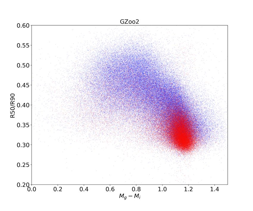
A&A 648, A122 (2021)

archive contains about 170 terabytes of information. Soon its          CANDELS survey and their detailed morphological features
successor, the Large Synoptic Survey Telescope (LSST), will            from the GZoo (clumpiness, bar instabilities, spiral structure,
acquire that quantity of data every five days (York et al. 2000).      merging). It allowed them to create a list of galaxies with fea-
It provided entry points for the computer scientists who want to       tureless disks at 1 ≤ z ≤ 3, which may represent “a dynamically
engage in astronomical research, and explains why big data min-        warmer progenitor population to the settled disk galaxies seen at
ing and machine learning methods are gaining such popularity:          later epochs”.
they are able to categorize celestial bodies in big data sets with          Kuminski & Shamir (2016) have generated a morphology
more accuracy than ever.                                               catalog of the SDSS galaxies with the Wndchrm image anal-
     In this context we review below several works where differ-       ysis utility using the nearest neighbor classifier. They pointed
ent approaches were developed and great efforts were made to           out that about 900 000 of the instances classified as spirals and
identify the morphological types of galaxies from the SDSS in          about 600 000 of those classified as ellipticals have a statisti-
the visual and in the automated modes.                                 cal agreement rate of about 98% with the GZoo classification.
     Ball et al. (2004) tested a supervised ANN for 50 mor-            Murrugarra & Hirata (2017) evaluated a convolutional neural
phological classifications and found that it can be used with-
                                                                       network to classify galaxies from the SDSS into two classes
out human intervention for the SDSS galaxies (correlations
                                                                       (ellipticals and spirals) by image processing, and attained an
between predicted and actual properties were around 0.9 with
rms errors on the order of 10%). de la Calleja & Fuentes (2004)        accuracy of 90–91%. Using the same machine learning tech-
developed a method that combines two machine learning algo-            nique, the convolutional neural network and especially the incep-
rithms: locally weighted regression and ANN. They tested it            tion method, Rahman & Azhari (2018) conducted classification
with 310 images of galaxies from the New General Catalogue             into three general categories: ellipticals, spirals, and irregulars.
and obtained an accuracy of 95.11% and 90.36%, respectively.           They used 710 images (206 E, 320 S p, 184 Irr) and obtained
Kasivajhula et al. (2007) explored support-vector machine, ran-        that images after processing showed a relatively low testing
dom forest, and naive Bayes algorithms as the galaxy image clas-       accuracy compared to those that did not undergo any form of
sifiers, and principal component analysis for the direct image         image processing. Their best testing accuracy was 78.3%.
pixel data compressing, but favored random forest. They cited               Supervised and unsupervised methods were both applied by
the opinion of several astronomers on the successful perspec-          Gauthier et al. (2016) to study the GZoo data set of 61 578 pre-
tive of galaxy classification by morphological features as “one        classified galaxies (spiral, elliptical, round, disk). They found
of the most cumbersome areas in celestial classification, and the      that the variation in galaxy images is correlated with brightness
one that has proven the most difficult to automate”. Neverthe-         and eccentricity, and that the random forest method gives the best
less, Andrae et al. (2010) applied a probabilistic classification      accuracy (67%); meanwhile, its combination with regression to
algorithm to classify the SDSS bright galaxies and obtained that       predict the probabilities of galaxies associated with each class
it produces reasonable morphological classes and object-to-class       can reach 94% accuracy. Beck et al. (2018) analyzed the inte-
assignments without any prior assumptions.                             gration of visual labeling and automated morphological assign-
     For the visual morphological classification conducted dur-        ment with random forest for more than 200 000 galaxies from
ing recent years, we note the following: Nair & Abraham (2010)         the GZoo2 project. They managed to show that such a combi-
prepared the detailed visual classifications for 14 034 galaxies       nation increases the binary classification rate with quite good
from the SDSS DR4 at z < 0.1, which can be used as a good              accuracy (93.1%), focusing on the velocity, one of the four Vs
training sample to calibrate the automated galaxy classification       of astronomical data (volume, variety, velocity, and value).
algorithms. Banerji et al. (2010) provided a significant study              The photometric and spectral parameters of each object,
where galaxies from the Galaxy Zoo Project1 formed a train-            as well as their images, are available through the SDSS web-
ing sample for morphological classifications of galaxies from the      site. It uses a well-known fact that galaxy morphological type
SDSS DR6 into three classes (early types, spirals, spam objects).      is correlated with several parameters, for example the color
These authors showed, at a high confidence level, that using a         indices, luminosity, de Vaucouleurs radius, and inverse concen-
set of certain galaxy parameters, a neural network can reproduce       tration index. In our series of works we have demonstrated the
human classifications to better than 90% for all these classes,        effectiveness of a combination of the visual classification and
and the Galaxy Zoo catalog (GZoo1) can serve as a training             the two-dimensional diagrams of color indices g − i and one
sample.                                                                of the parameters mentioned above (Vavilova et al. 2009, 2015;
     Hundreds of thousands of volunteers were involved in the          Melnyk et al. 2012; Dobrycheva & Melnyk 2012). Specifically,
Galaxy Zoo project (GZoo) to make a visual classification of           using the color indices versus inverse concentration index dia-
a million galaxies in the SDSS (Lintott et al. 2008). Most             grams for each galaxy with radial velocities 3000 < V <
of their results have found good scientific applications. For          9500 km s−1 from the SDSS DR5, we obtained criteria for sep-
example, using the raw imaging data from SDSS that was                 arating the galaxies into three classes, namely (E) early types–
available in the GZoo1, and the handpicked features of galax-          elliptical and lenticular, (S ) spiral S a − S cd, and (LS ) late spiral
ies from the SDSS, Kates-Harbeck (2012) applied a logistic             S d − S dm and irregular Im/BCG galaxies (Melnyk et al. 2012).
regression classifier and attained 95.21% classification accuracy.          Making a ternary automated morphological galaxy classifi-
Willett et al. (2013) issued a new catalog of morphological            cation we attained good accuracy: 98% for E, 88% for S, and
types from the GZoo2 Project in synergy with the SDSS DR7,             57% for LS . We applied this approach based on the photometric
which contains more than 16 million morphological classifica-          data alone (multi-parametric diagrams) to classify a sample of
tions of 304 122 galaxies and their finer morphological features       316 031 SDSS galaxies at 0.003 ≤ z ≤ 0.1 from the SDSS DR9
(bulges, bars, and the shapes of edge-on disks as well as param-       (142 979 E, 112 240 S , 60 812 L; Dobrycheva 20132 ). The cri-
eters of the relative strengths of galactic bulges and spiral arms).   terion was determined visually by the graph of the relationship
Simmons et al. (2017) cross-verified 48 000 galaxies from the
                                                                       2
                                                                         http://leda.univ-lyon1.fr/fG.cgi?n=hlstatistics&a=
1
    http://data.galaxyzoo.org                                          htab&z=d&sql=iref=52204

A122, page 2 of 14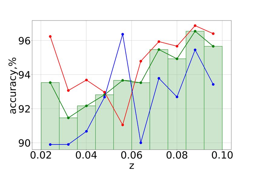
I. B. Vavilova et al.: Machine learning for the galaxy morphological classification

between these two values. In each graph we indicated the regions         binary morphological classification. Mittal et al. (2020) intro-
where there are a maximum number of galaxies of morphologi-              duced the data augmentation-based MOrphological Classifier
cal types E, S , and LS and a minimum number of other morpho-            Galaxy using Convolutional Neural Networks (daMCOGCNN)
logical types. At that time, we used the training sample as a test       and obtained a testing accuracy of 98%. Their data sets of 4614
sample, which means that the actual accuracy was at least a few          images were collected from SDSS Image Gallery, Galaxy Zoo
percentage points lower. A more detailed explanation is given by         challenge, and Hubble Image Gallery.
Dobrycheva et al. (2018).                                                     It can be seen that, in general, the implemented methods with
     The ternary classification is a partial case of decision tree       CNN provide accuracy around 98% for the morphological clas-
classifier and provides an accuracy level of morphological classi-       sification of galaxies. However, they require imaging data with
fication that is not very high. We tried to use other more sophisti-     a good resolution, and work well for nearby galaxies. On the
cated machine learning methods and to compare them. In works             contrary, in our classifiers we use easily observed photometric
by Dobrycheva (2017), the results on a binary morphological              parameters, which could even be defined for distant galaxies.
classification of this sample using software with an open-source              The above brief discourse into the history of the automated
KNIME Analytics Platform ver. 3.5.0 were presented, and three            morphological classification of various galaxy samples from a
machine learning methods were compared: naive Bayes, random              homogeneous Sloan Digital Sky Survey shows that classifica-
forest, and support-vector machine based on WEKA 3.7 soft-               tion accuracy (success rate) depends not only on the obvious
ware and neural networks (RProp MLP). It turned out that the             factors such as the quality of the data (photometric, image, spec-
random forest method provided the highest accuracy: 91% of               tral) or human labeling, but also on the applied machine learn-
galaxies were correctly classified (96% for E type and 80% for           ing methods. Moreover, it is important to discuss not only the
L type).                                                                 effectiveness of the methods, but also the problem points that
     The higher rate of morphological classification was accessed        are hidden in general statistics of a success rate. Specifically,
with convolutional neural network (CNN) when the imaging                 they are directly related to the evolutionary features of galaxies.
data was analyzed. We note some recent works where galaxy                Here the developed tools and catalogs based on the photometric
samples in the Local Universe were studied.                              data augmentation may serve an essential role as training sam-
     Sreejith et al. (2018) exploited 7528 galaxies from the             ples for the data analysis of upcoming biggest surveys as LSST
Galaxy and Mass Assembly (GAMA) survey with 0.002 < z <                  and Euclid.
0.06. These galaxies were previously visually classified indepen-             This work deals with the automated morphological classifi-
dently by three classifier teams. The statistical machine learn-         cation of the low redshift galaxies from the SDSS DR9. We used
ing algorithms were trained on a set of 6022 objects (80% of             the cosmological WMAP7 parameters Ω M = 0.27, ΩΛ = 0.73,
the data set) using ten independent distance parameters. These           Ωk = 0, H0 = 0.71 and set the following tasks:
algorithms were subsequently tested on the remaining 20% of                   – to verify various machine learning methods and to select
the data set to classify them into five galaxy types: elliptical,        most effective among them for classifying the morphological
little blue spheroid, early-type spirals (S0-SBa), intermediate-         types of galaxies at z < 0.1 from the SDSS DR9;
type spirals (Sab-SBcd), and late-type spirals–irregulars (Sd-                – to determine the margins where the automated morphology
Irr). Their results were as follows: support-vector machine –            classification based on the photometric parameters of galaxies
75.8%, neural networks – 76.0%, classification trees – 69.0%,            gives the best result, e.g. morphological peculiarities, at different
and classification trees with random forest – 76.2%. Cheng et al.        redshifts;
(2020) used the Dark Energy Survey data combined with human                   – to reveal typical problem points of the automated morpho-
labeling from the GZoo1 project to compare the effectiveness             logical classification based on the photometric data and human
of several machine learning methods, among which CNN, k-                 labeling;
nearest neighbors, logistic regression, support-vector machine,               – to apply the developed criteria for the automated morpho-
random forest, and neural networks. These authors obtained that          logical classification of galaxies at z < 0.1 from the SDSS DR9
CNN is the most successful method for the binary morphologi-             with unknown morphological types.
cal classification dealing with galaxy images; using a sample of         We organized the paper as follows. Section 2 deals with galaxy
∼2800 galaxies at z < 0.25, they attained an accuracy of ∼99%.           samples. Section 3 describes the studied machine learning
     Barchi et al. (2020) produced a catalog with morphologi-            methods (naive Bayes, logistic regression, k-nearest neighbors,
cal data for 670 560 galaxies at 0.03 < z < 0.1, where the               random forest, and support-vector machine) and the setting
input data were taken from SDSS-DR7 (Petrosian magnitude in              parameters used in each method. The results are presented in
r-band brighter than 17.78, and |b| > 30◦ ). They used traditional       Sect. 4. In the discussion we raise questions about several prob-
machine learning (TML) and deep learning (DL) approaches                 lem points of the supervised machine learning methods for the
to distinguish elliptical (E) from spiral (S ) galaxies. These           automated galaxy morphological classification (Sect. 5.1) and
authors presented a non-parametric galaxy morphology system,             compare the effectiveness of different methods (Sect. 5.2). Con-
named CyMorph, which determines concentration (C), asym-                 cluding remarks are highlighted in Sect. 6.
metry (A), smoothness (S), entropy (H), and gradient pattern                  Our other approach dealing with the deep learning similarity
analysis (GPA) metrics. All the studied TML methods (decision            to define morphological features of galaxies from this studied
tree, support-vector machine, and multi-layer perceptron) pro-           sample is described in the next paper by Khramtsov et al. (2020).
duced a 98% overall accuracy. Despite an imbalance of types
in the training set (S galaxies, 87%, and E galaxies, 13%) at
least 95% accuracy and 96% recall for E systems were attained.           2. Galaxy samples from the SDSS DR9 for the
Since S galaxies constitute most of the training set, it is not sur-        automated morphological classification
prising that accuracy and recall were 99%, establishing a model          2.1. Galaxy sample
with 99% overall accuracy for this data set. In general, the CNN
method (GoogLeNet Inception) with the imbalanced data sets               A preliminary sample of galaxies at z < 0.1 with the abso-
and 22-layer network resulted in 98.7% overall accuracy for              lute stellar magnitudes −24m < Mr < − 13m from the SDSS DR9

                                                                                                                           A122, page 3 of 14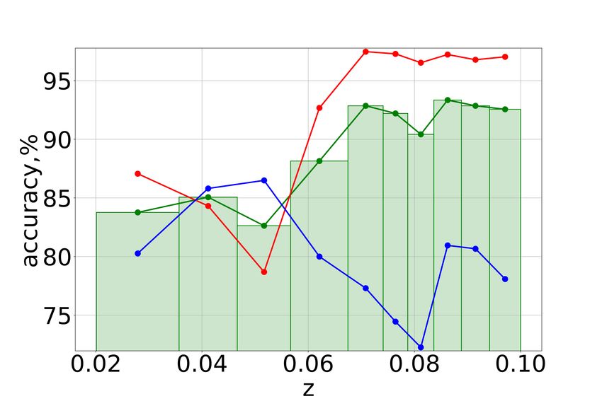
A&A 648, A122 (2021)

         0.60

         0.55

         0.50

         0.45
   R50/R90

         0.40

         0.35

         0.30

         0.25

         0.20
            0.0   0.2   0.4     0.6       0.8   1.0   1.2     1.4
                                      Mg − Mi
Fig. 1. Diagram of color indices g − i and inverse concentration indexes
R50/R90 of the training sample (6163 galaxies randomly selected with
different redshifts and luminosities from the SDSS DR9). The visually
classified galaxies (human labeling) of early E − S 0 types are shown in
red, and the late Sa − Irr types in blue.

contained ∼724 000 galaxies. Following the SDSS recommen-
dation, we input limits mr < 17.7 by visual stellar magnitude
                                                                           Fig. 2. Distribution of the morphological types (early in red, late in blue)
in r-band to avoid typical statistical errors in spectroscopic flux.       depending on the photometric parameters: (left panel) color indices
After excluding the images with duplicates of the same galaxy              Mg − Mi , (right panel) inverse concentration index R50/R90) for the
and artificial objects, the final sample contained N = 316 031             training sample of 6163 galaxies as in Fig. 1.
galaxies. To clear the sample from segmented images of the same
galaxy, we used our code based on the minimum angle distances
between such SDSS objects.                                                 features as much as possible, allowing us to generalize and to
    The absolute stellar magnitude of the galaxy was obtained              build the model for predicting the target variables (see, e.g.,
by the formula                                                             Kremer et al. 2017). That is why our first step before applying
                                                                           the machine learning methods was to compose a good quality
Mr = mr − 5 · lg(DL ) − 25 − Kr (z) − extr ,
                                                                           training sample.
where mr is the visual stellar magnitude in r-band, DL the lumi-                We visually identified the morphological types (E and L)
nosity distance, extr the Galactic absorption in r-band in accor-          of 6163 galaxies from the sample described in Sect. 2.1, which
dance to Schlegel et al. (1998), Kr (z) the k-correction in r-band         were randomly selected at different redshifts and with different
according to Chilingarian et al. (2010), Chilingarian & Zolotukhin         luminosity. This is ∼2% of the total number of the studied galaxy
(2012).                                                                    sample. We used images from multiple bands for the visual clas-
   The color indices were calculated as                                    sification.
                                                                                To eliminate the human error factor, cross-validation of the
Mg − Mi = (mg − mi ) − (extg − exti ) − (Kg (z) − Ki (z)),                 same galaxies for their types and morphological features was
                                                                           performed by the authors of this paper. To label the galaxy
where mg and mi are the visual stellar magnitude in g- and                 types at different redshifts in the case of disputable visual clas-
i-band; extg and exti the Galactic absorption in g- and i-band; and        sification, we took into account their spectral data for addi-
Kg (z) and Ki (z) the k-correction in g- and i-band, respectively.         tional clarification (e.g., the presence of a strong emission line
    A ternary morphological classification with the method of              Hα for the spiral galaxy SDSS J124332.66+172004.3 at z =
multi-parametric diagrams (in-box classification) does not attain          0.02 and an absorption line Hβ for the elliptical galaxy SDSS
a reasonable accuracy to classify spiral galaxies of S a−S cd type         J155947.57+263334.4 at z = 0.09).
(see Sect. 1, and Dobrycheva et al. 2015, 2018; Vavilova et al.                 Using one of the three color indices and such parame-
2020a). To verify the various supervised machine learning meth-            ters as the inverse concentration index, absolute stellar magni-
ods we decided to provide a binary automated morphological                 tude, de Vaucouleurs radius, and scale radius (color − R50/R90,
classification: early-type galaxies E, from ellipticals to lenticu-        color − Mr , color − deVRadr , and color − expRadr diagrams,
lars; late-type galaxies L, from S0a − Sdm to irregular Im/BCG             respectively), it is possible to carry out a reliable preliminary
galaxies.                                                                  morphological classification without invoking visual inspection.
                                                                           The dependence of the color indices and the parameter R50/R90
2.2. Training samples                                                      gives the best fit because the parameter values do not depend on
                                                                           the radial galaxy velocity and because the selection effects are
The supervised machine learning methods are used in the search             avoided (Dobrycheva & Melnyk 2012). As an example, see the
for a relationship between the input and output data, in our case,         diagram of inverse concentration indexes R50/R90 as a function
between features of galaxies (photometric parameters) and their            of color indices g − i for 6163 galaxies of the training sample,
morphological types. A training sample should represent these              which is shown in Fig. 1. It demonstrates a good separation into
A122, page 4 of 14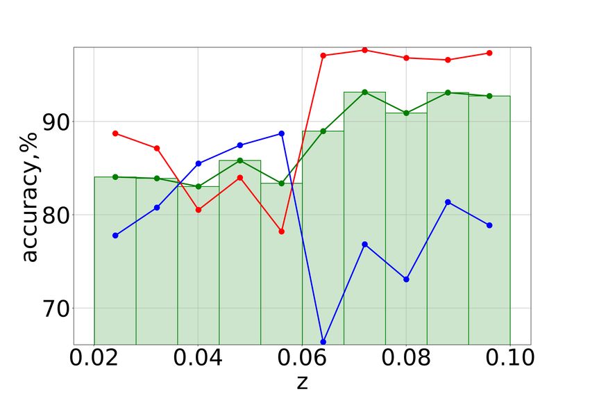
I. B. Vavilova et al.: Machine learning for the galaxy morphological classification

the early and late galaxy types (Fig. 2) and also reveals the well-        Bayes computes the posterior probability for each class G:
known effect of color indices bimodality (Balogh et al. 2004).                      p(G) ni=1 p(xi |G)
                                                                                        Q
The overlap of morphological types in the range of Mg − Mi from            p(G|X) =                    .
1.1 to 1.3 is still substantial and will be discussed in Sect. 5.                         p(X)

                                                                           3.2. Random forest
3. Supervised machine learning methods and
                                                                           The random forest (RF) classifiers works as follows. The training
   morphological classification                                            sample contains N objects whose dimension of objects feature is
The learning can be supervised, semi-supervised, unsupervised,             M (Mu , Mg , Mr , Mi , Mz , Mu − Mr , Mg − Mi , Mr − Mz , inverse con-
and reinforced (Burkov 2019). In our work we only used the                 centration indexes R50/R90 √ to the center) and the parameter m
supervised methods where the data set is a collection of the               is given (usually m = M) as an incomplete number of traits
labeled examples (xi , yi )i=1N
                                 .                                         for training. Then we build the committee tree; the most com-
     In our case each element xi among N is a galaxy feature               mon way is as follows. First, we generate a random subsample
vector, where each dimension j = 1, . . . , D contains a value             with size N likely in the training sample. Thus, some objects
that describes yi . That value is called a feature and is denoted          will hit two or more times, and on average N(1 − 1/N)N , and
as x( j) . For instance, if each example x in our collection repre-        approximately N/e objects will not hit at all. Next, we construct
sents a galaxy, then the first feature, x(1) , could contain abso-         the decision tree that classifies the objects in this subsample.
lute magnitude Mu , the second feature, x(2) , could contain color         The next node of the tree in the process of creating will use not
indices Mu − Mr , and x(3) could contain the inverse concentra-            all M objects features, but only m, which are randomly chosen.
tion index R50/R90. Summing up, there are absolute magnitudes              Finally, we develop the tree up to the complete exhaustion of the
Mu , Mg , Mr , Mi , Mz ; color indices Mu − Mr , Mg − Mi , Mr − Mz ;       subsample.
and inverse concentration indexes R50/R90 to the center. For all               The classification of objects is conducted by voting: each tree
examples in the data set, the feature at position j in the feature         of the committee puts the object into one of the classes, and the
vector always contains the same kind of information. This means            class wins if it has the most significant number of trees voted
that if xi(2) contains color indices Mu − Mr for some example xi ,         (Breiman 2001). In our case the forest consisted of 500 trees and
then xk(2) will also contain color indices Mu − Mr in each example         the maximum depth of the tree was equal to 11.
xk , k = 1, . . . , N. The label yi can be either an element belonging
to a finite set of classes 1, 2, . . . , T , or a real number, or a more   3.3. Support-vector machine
complex structure, like a vector, a matrix, a tree, or a graph. In
our work we only have two classes, E and L, where E means the              We get a training data set of n points of the form
early-type galaxy and L means the late morphological type.                 (x1 , y1 ), . . . , (xn , yn ), where yi is either 1 or −1 (in our work it is
     The goal of a supervised learning algorithm is to use the data        E or L morphological type of the galaxy). Each point indicates
set to produce a model that takes a feature vector x as input, and         to which type the point xi belongs (set of attributes of galax-
outputs information that allows us to deduce the label for this            ies). Each xi is a p-dimensional real vector. We should find the
feature vector. For instance, the model with a data set of galaxies        “maximum-margin hyperplane” that divides the group of points
could take a feature vector describing the morphological type of           xi , for which yi = 1, from the group of points, for which yi = −1
galaxy as the input information and a probability that the galaxy          is defined in such a manner that the distance between the hyper-
has E or L morphological type as the output information.                   plane and the nearest point xi from either group is maximized.
     Using the Scikit-Learn machine learning library (ver. 0.2.2           Any hyperplane can be written as the set of points xi satisfy-
for the Python programming language (Pedregosa et al. 2011),               ing wi xi − b = 0, where wi is the normal vector (not necessarily
which is a simple tool for data mining and data analysis (see,             normalized) to the hyperplane. It is more likely Hesse’s normal
e.g., Ivezic et al. 2014), we trained naive Bayes, random forest,          form, except that wi is not necessarily a unit vector. The param-
support-vector machine, k-nearest neighbors, and logistic regres-          eter kwk
                                                                                  b
                                                                                       determines the offset of the hyperplane from the origin
sion. To train the classifier we used the absolute magnitudes              along the normal vector w (VanderPlas 2016; Cortes & Vapnik
Mu , Mg , Mr , Mi , Mz ; color indices Mu − Mr , Mg − Mi , Mr − Mz ;       1995).
and the inverse concentration index R50/R90 (Sect. 2.2).                         We used the support-vector machine (SVM) with radial basis
                                                                           function kernel without limit on the number of iterations until
                                                                           the condition of the solution is fulfilled. The inverse of regular-
3.1. Naive Bayes                                                           ization strength index C was equal to 78 (smaller values specify
The naive Bayes classifiers are based on the Bayes theorem and             stronger regularization). The parameter gamma was defined as
conditional independence of the features to calculate the prob-            “scale” by default.
ability of class G (in our case it is a morphological type of
galaxies) with a given feature vector (set of galaxy attributes)           3.4. K-nearest neighbors
X = (x1 , . . . , xi ):
                                                                           The classifier based on k-nearest neighbors (k-NN) is an example
                                                                           of the most straightforward machine learning algorithm. It does
           p(G)p(X|G)                                                      not create class-dividing functions, but remembers the position
p(G|X) =              .
              p(X)                                                         of training sample objects in the hyperspace of features. This
                                                                           method’s disadvantage is that its productivity linearly depends
    If we accept the conditional independence assumption,                  on the size of the training sample, the dependence on metrics,
instead of computing the class-conditional probability for each            and the difficulty in selecting statistical weight. To implement
combination of X, we only have to estimate the conditional prob-           this method it is enough to choose the number of neighbors
ability of each xi , given G. To classify a test record, the naive         (k, the distance metric), find the k-nearest neighbors in this
                                                                                                                                   A122, page 5 of 14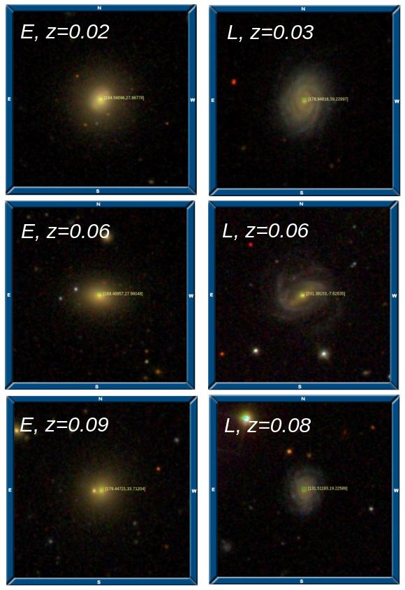
A&A 648, A122 (2021)
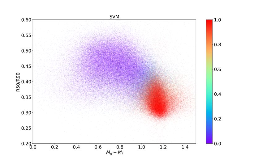
Fig. 3. Diagram of color indices g − i and inverse concentration indexes
R50/R90 of 316 031 galaxies at z < 0.1 from the SDSS DR9 after
applying the support-vector machine (SVM) method: red for early E
types (from elliptical to lenticular) and blue for late L types (from S0a
to irregular Im/BCG). The color bar from 0 to 1 shows the SVM prob-
ability to classify galaxy as late to early morphological types.
Table 1. Accuracy (in %) of the supervised machine learning methods
for the automated binary morphological classification of galaxies from
the SDSS DR9 at z < 0.1 (total, for early E and late L morphological
types, rms error)
Fig. 4. Distribution of the morphological types (early in red, late in blue)
in dependence on the color indices Mg − Mi (top) and inverse concentra-
Classifier vs. accuracy Total E type L type Error
tion index R50/R90 (bottom) for the main sample of 316 031 galaxies
Naive Bayes 89.0 92.0 82.0 ±1.0 as in Fig. 3.
K-nearest neighbors 94.5 93.9 95.8 ±0.6
Logistic regression 94.9 96.8 91.1 ±0.6
Random forest 95.5 96.7 92.8 ±0.3 returned by the model for input x is closer to 0, then we assign a
Support-vector machine 96.4 96.1 96.9 ±0.6 negative label to x; otherwise, the example is labeled as positive.
One function that has such a property is the standard logistic
function (also known as the sigmoid function):
metric, and assign to the object the class of the largest number
of his neighbors. This method can be used not only for binary 1
f (x) = .
classification. In this case, the neighbors can be assigned a sta- 1 + e−x
tistical weight of 1/d, where d is the distance in the features’
hyperspace. This meter is also sensitive to normalization, as all The inverse of regularization strength index C in our work
features must make the same contribution to the distance esti- was equal to 6.
mation. Finding the number k is important because it allows
us to describe the model avoiding retraining and undertraining 4. Results
(Raschka 2015). Depending on the metric of space, the distance
will be determined in different ways, for example, in Euclidean We used the method of k-folds validation to estimate the accuracy.
space: Specifically, we divided the sample into randomly selected five
sX batches, one by one, four of which served as the training and one
di, j = |xi − x j |2 . as the test sample. This procedure was repeated five times, and
k
the classification accuracy was defined as the average of the test
samples. We set aside 20% of the training sample to verify the
The setting of weights for neighbors is not significant in the case accuracy of predicting morphological types with Python. As the
of overnumbered galaxies in the training sample. We got the best next step, we used the k-folds validation to predict the types in
results if this classifier made a decision based on the 11 nearest this delayed valid sample used to verify the method’s accuracy.
neighbors. We consider the accuracy change as a function of the sample
size: if this function attains a higher level, an existing set of the
3.5. Logistic regression training data is enough. However, if the accuracy continues to
grow, most likely it will not hurt to increase the amount of train-
In logistic regression (LR) we can model a morphological type ing data. To evaluate the accuracy of the methods, we performed
of galaxy yi as a linear function of xi . However, with a binary the following procedures for a test sample of N = 6163 galaxies
yi this is not straightforward because wxi + b is a function that with Python software. First we divided the training sample into
spans from minus infinity to plus infinity, while yi has only two subsamples, changing the proportions between the sizes of train-
possible values (Burkov 2019; Raschka 2015). For binary mor- ing and test samples. Then we randomly repeated the procedure
phological classification we define a negative label as 0 and a ten times for the formation of each subsample. Next we ran these
positive label as 1, and we would need to find a simple continu- subsamples with the Scikit-learn machine learning with Python
ous function whose codomain is (0, 1). In this case if the value for all the methods and determined their accuracy.
A122, page 6 of 14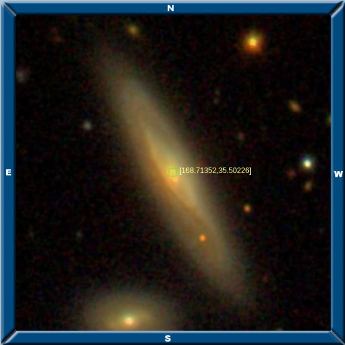
I. B. Vavilova et al.: Machine learning for the galaxy morphological classification

Fig. 5. Verification of whether there are enough galaxies in a training
sample to build a machine learning model. The green line (support-
vector machine), the red line (random forest), the pink line (logistic
regression), the blue line (k-nearest neighbors), and the orange line
(naive Bayes) show the average accuracy of ten repetitions of the eval-
uation procedure in Scikit-learn machine learning with Python.

    It turned out that support-vector machine and random forest
classifiers provide the highest accuracy of the automated binary
galaxy morphological classification: 96.4% correctly classified
(96.1% E and 96.9% L) and 95.5% correctly classified (96.7%
E and 92.8% L), respectively (Table 1).
    As a result, using the data on the absolute stellar magnitudes,
color indices, and inverse concentration indexes, and coaching
by support-vector machine classifier to galaxies with visual mor-
phological types, we applied these criteria to the studied sample
of N = 316 031 galaxies with unknown types. We got the fol-
lowing classifications: 139 659 early E types and 176 372 late L
morphological types (Fig. 3). The diagrams are given in (Fig. 4).
    The verification of the methods whether there are enough
galaxies in a training sample to build a machine learning model
is demonstrated in Fig. 5.
    The results obtained for each method’s ability to accurately
determine the morphological type of the galaxy can be easily
illustrated graphically (Fig. 6). We consider the probability of
finding the position of each galaxy (point on the graph) on the
hyper-plane of two parameters (inverse concentration index and
one of the color indices) for each of the used machine learning
methods (Table 1). In each of the panels in Fig. 6 the input data
from the training sample is embedded as in Fig. 1 (6163 galaxies
randomly selected with different redshifts and luminosity from
the SDSS DR9): red corresponds to the early morphological
type, blue to the late-type galaxies. This visualization helps to
analyze a tuning of the studied machine learning algorithms to
classify the galaxy types.
                                                                          Fig. 6. Probability distribution for finding the position of each galaxy on
5. Discussion                                                             the hyper-plane of two photometric parameters R50/R90 vs. Mg − Mi .
                                                                          The training sample (Fig. 1) is embedded in each of the panels, which
Various machine learning methods are helpful not only for the             shows the effectiveness of the methods used to classify galaxy types at
classification of objects by morphological features of celestial          z < 0.1. The accuracy of each applied machine learning method for the
bodies. They are sufficient for reconstruction of the Zone of             two-parameter classification is written in the left corner of each panel.
Avoidance (Vavilova et al. 2018), finding gamma-ray sources for
the upcoming Cherenkov Telescope Array (Bieker 2018), spatio-
temporal data (Wang et al. 2019), classification of variable stars        photometric redshift estimation (Mu et al. 2020), prediction of
light curves (Kim & Bailer-Jones 2016) and light-curve shape              galaxy halo masses (Calderon & Berlind 2019), gravitational
of a Type Ia supernova (Stahl et al. 2020), determination of              lenses search (Khramtsov et al. 2019a), automating discovery
the distance modulus for local galaxies (Elyiv et al. 2020) and           and classification of variable stars (Bloom et al. 2012), and for
                                                                                                                                A122, page 7 of 14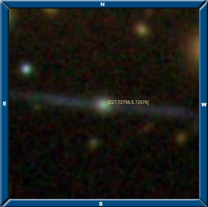
A&A 648, A122 (2021)

analyzing huge observational surveys, for example the Zwicky
Transient Facility (Mahabal et al. 2019), or finding planets and
exocomets from the Kepler and TESS surveys (Kohler 2018).
     Among other recent examples, we also note the determina-
tion of physical properties of galaxies (density, metallicity, col-
umn density, ionization) from their emission-line spectra with
support-vector machine algorithms employed and developed in
a new GAME numerical code by Ucci et al. (2017); predic-
tion of the HI content of massive galaxies at z < 2 based on
optical photometry data (SDSS) and environmental parameters,
which was performed by Rafieferantsoa et al. (2018) with regres-
sors and deep neural network (see also examples of applica-
tions of the AstroML Python module 5 for the large-scale obser-
vational extragalactic surveys3 ). In addition to the traditional
approach for classifying the galaxy types automatically in the
optical range, the machine learning methods also demonstrate a
strong utility for classifying the radio galaxy types and peculiar-
ities (Aniyan & Thorat 2017; Alger et al. 2018; Wagner et al.
2019; Lukic et al. 2019; Ralph et al. 2019).
     When implementing machine learning methods for different
astronomical tasks it is very useful to discuss their advantages
and problem points, data quality regularity, and flexibility of the
classification pipeline.

5.1. Several problem points of the supervised machine
     learning methods and data quality for the automated
     morphological classification of galaxies from the SDSS
The main problems of machine learning related to the morpho-
logical classification can be divided into two categories. The first
concerns a sample preparation, which includes determining the
parameters that are the best for dividing objects into classes,
selecting a homogeneous data set for classification parameters,
creating a sub-directory for training algorithms, cleaning the         Fig. 7. Estimation of the relative importance of some photometric
sublist of undesired (misclassified) objects, determining the most     parameters for the random forest classifier of galaxies from the SDSS.
effective methods for the decision making, and selecting the best      The training sample contains 11 000 galaxies. Parameters with the
machine learning features to build training sample. The second         highest values correspond to the most significant parameters: deVABu ,
category includes problems related to the individual peculiarities     deVABg , deVABr , deVABi , deVABz for the de Vaucouleurs radius fit
of selected objects and the quality of the image, the photometry,      b/a in different bands; expABu , expABg , expABr , expABi , expABz
and the spectrum galaxy data.                                          for the exponential fit b/a in different bands; z for redshift; Mu − Mr ,
                                                                       Mg − Mi , Mr − Mz for the color indices; Mu , Mg , Mr , Mi , Mz for the
    Selection of the best parameters of machine learning for           absolute magnitudes, and R50/R90 for the inverse concentration index
training. To determine the training parameters, we need the rela-      to the center.
tionship between the model’s accuracy in training and test sam-
ples. In other words, we must choose parameters in such a way          photometry parameters, we need (a) to create a small homoge-
that (a) the accuracy of the test sample is as high as possible,       neous galaxy sample for training, where all the data sets have
(b) the accuracy of the methods applied to the training sample         certain types available in the database; (b) to test these param-
should not attain 100% value to avoid overfitting (see, e.g., the      eters using, for example, the Fisher method for evaluating the
figures on the prediction accuracy by Vasylenko et al. 2019),          significance of these features (Fig. 7); and (c) to determine the
and (c) the difference in accuracy between the test and training       distribution of galaxies of different types at different redshifts
samples is minimal. However, these requirements do not always          selecting sets of benchmarks by analyzing slices for one or sev-
coincide simultaneously. So, the averaged values of the training       eral parameters.
and test samples’ accuracy ratios should be analyzed for a larger          We can see in Fig. 7 that the higher relative importance
number of cycles to determine the best parameters.                     among photometric parameters, which correlate with morphol-
    To select the optimal parameters, we applied the Grid-             ogy, have the color indices Mu − Mr , Mg − Mi , Mr − Mz , and
SearchCV tool from the Scikit-learn library and the balanced           inverse concentration index to the center R50/R90. Other fea-
class scales for the classifiers, except for the Gaussian naive        tures such as absolute magnitudes Mu , Mg , Mr , Mi , Mz ; expo-
Bayes. The balanced mode in models uses the values to auto-            nential fits b/a in different bands expABu , expABg , expABr ,
matically adjust the weights, which are inversely proportional to      expABi , expABz ; de Vaucouleurs radius fits b/a in differ-
the input data’s class frequencies.                                    ent bands deVABu , deVABg , deVABr , deVABi , deVABz ; and
   Features of galaxies, which are the best fitted for the             redshift z are less important. We verified that inclusion of
morphology classification into types. To determine these               exponential fits, de Vaucouleurs radius fits, and redshifts as the
                                                                       additional features of galaxies does not increase the accuracy
3
    https://www.astroml.org                                            of machine learning methods applied to the training sample of
A122, page 8 of 14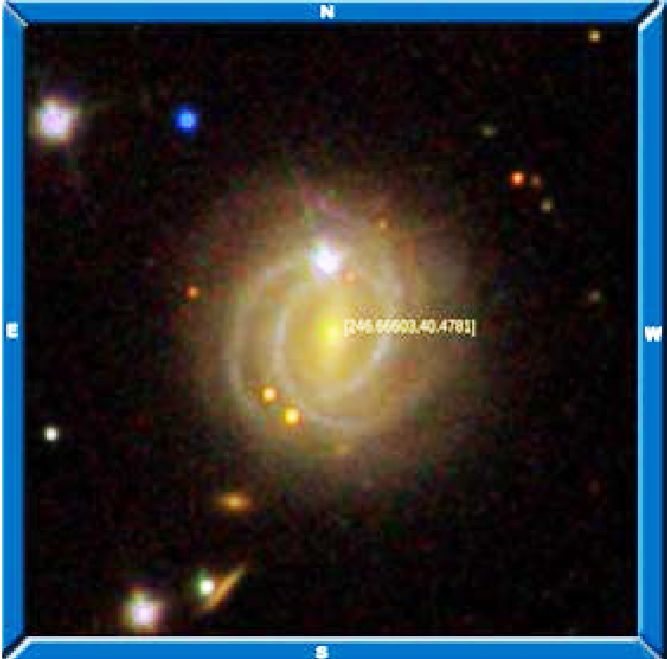
I. B. Vavilova et al.: Machine learning for the galaxy morphological classification

                                                                            (a) Interacting galaxy             (b) Background galaxy
                                                                            RA=206.6429, DEC=60.3069,          RA=205.6965, DEC=26.3649,
                                                                            z=0.072                            z=0.064

                                                                            (c) Stars overlapping the galaxy   (d) Artifacts
                                                                            image RA=246.6660,                 RA=252.1989, DEC=26.9678,
                                                                            DEC=40.4781, z=0.034               z=0.054

Fig. 8. Examples of images of galaxies from the SDSS DR9 at z < 0.1
classified correctly as early E and late L types.
                                                                            (e) Gravitational lens             (f) Face-on spiral galaxy with
                                                                            RA=233.9972, DEC=4.6089,           a bright nucleus, RA=176.5507,
                                                                            z=0.032                            DEC=20.3916, z=0.023
11 301 galaxies. This is 83.6% when they are also included (see
Table 2 for SVM classifier). We did not use them, and this
allowed us to also reduce the computational cost.

    Image–photometry–spectrum quality of the data. The
examples of images of galaxies, which are correctly classified
into early and late types, are given in Fig. 8. The problem
points of the SDSS galaxy data, which led to their morphol-
ogy misclassification, are as follows (Fig. 9): (1) interacting
galaxies (Fig. 9a), (2) background galaxy (Fig. 9b), (3) stars
covering the galaxy image (Fig. 9c), (4) artifacts (diffraction,
satellites) (Fig. 9d), (5) red spiral galaxies or 6) galaxies with          (g) Ultra-flat spiral galaxy       (h) Edge-on spiral galaxy with
a bright nucleus (Fig. 9f), (7) bad background, (8) dim objects             RA=227.72756,                      a bright bulge, RA=168.71352,
                                                                            DEC=5.72077, z=0.02211             DEC=35.50226, z=0.021
(low signal-to-noise ratio), (9) face-on and edge-on galaxies
(Figs. 9g, h), and 10) “false” objects, such as gravitational lenses.    Fig. 9. Examples of images of galaxies from the SDSS DR9 at z <
(Fig. 9e). These objects can be simply identified and deleted            0.1, when the morphological types can be misclassified in the machine
at the step of building the finest quality training sample (see          learning pipeline.
Sect. 2.2).
    We also used the spectra in combination with image and
photometry data in several questionable cases for the face-on                Human labeling (HL) was the only way to determine the
spirals, lenticulars, and E0-E1 type galaxies to train classifiers       morphological types of galaxies until the advent of the big data
(for instance, SDSS J124332.66+172004.3, SDSSJ155947.57+                 era (see, e.g., references on the early and modern galaxy surveys
263334.4). Nevertheless, we conclude that such morphologically           and catalogs in our review Vavilova et al. 2020b).
misclassified objects contribute ∼1% error in the classification of          Among the works with 100% successful visual inspection
a general galaxy sample (see also Kasivajhula et al. 2007).              that led to the discovery and cataloging of galaxies with types
                                                                                                                               A122, page 9 of 14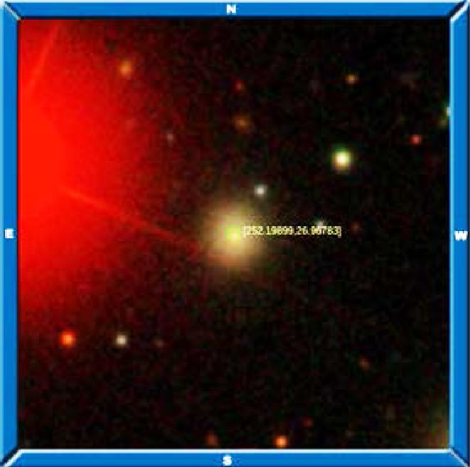
A&A 648, A122 (2021)

Fig. 10. Confusion matrices after cross-matching of the studied samples
and GZoo2: HL – 4834 galaxies from training sample; SVM – ∼173 000
galaxies with the support-vector machine classifier: E, early-type galax-
ies; L, late-type galaxies; green, galaxies that have the same type in both
samples; red, galaxies where the types did not match.

that do not fit into classical morphological schemes are on the
interacting galaxies, galaxies with excess radiation in certain
spectral ranges, compact galaxies, galaxies of low and high
surface brightness, and others. For example, the use of the
catalogs of galaxies of low surface brightness (dwarfs and nor-
mal) based on visual inspection, even in the absence of data on
redshifts, made it possible to determine their role in the large-             Fig. 11. Distribution of ∼173 000 galaxies at z < 0.1 from the GZoo2
scale structure of normal galaxies in the Local Supercluster (see,            on the plane of photometric parameters of color indices g − i and inverse
e.g., Karachentseva & Vavilova 1994, 1995; Lisker et al. 2008;                concentration indexes R50/R90: early (red) and late (blue) morpholog-
Miskolczi et al. 2011; Paudel et al. 2018).                                   ical types are from the GZoo2 labeling.
     Even though visual inspection of galaxies is becoming pro-
hibitively time-consuming, the human labeling method remains
a necessary classifier of morphological types both when compil-
ing small samples of galaxies for solving various astrophysical
and astrochemical tasks (Pilyugin et al. 2018; Du et al. 2019;
Martin et al. 2020), and for building the training samples in tasks
of automated classification.
     Under these circumstances, we paid special attention to the
labeling and cross-validation of the same galaxies from the train-
ing sample. As we mentioned in Sect. 2.2, it was performed by
the authors.
     At the same time, following works by Willett et al. (2013),
Kuminski & Shamir (2016), and Beck et al. (2018) mentioned
in the Introduction, we compared our results and the debi-
ased GZoo2 data trying to take into account all the differ-
ences in approach to the labeling of morphological features of
galaxies.
     With this aim, we cross-matched 316 031 galaxies and their
morphological types obtained by the support-vector machine
with the GZoo2 data, which yielded ∼173 000 galaxies (SVM
and GZoo2 in Fig. 10). The accuracy is 69.7%. We also cross-
matched 6 163 galaxies from the training sample (HL in Fig. 10)
with the GZoo2 data, which yielded 4834 common galaxies. The
accuracy is 72.2%. The coordinate error for cross-matching in
both cases is dRA,Dec ≤ 100 .
     The similarity of accuracy values indicates, first of all,
that both support-vector machine and human labeling manage
                                                                              Fig. 12. Distribution of the morphological types (early, red; late, blue)
equally well when we use the photometry-based approach to                     in dependence on the photometric parameters: color indices Mg − Mi
compare our binary classification with the GZoo2 data. Second,                (top) and inverse concentration index R50/R90 (bottom) for the GZoo2
the Fig. 10 highlights a different approach to the visual labeling            sample of ∼173 000 galaxies, as in Fig. 11.
of galaxies by morphological types for our galaxy sample and
the GZoo2 sample. The confusion matrices allow us to under-
stand the differences in this labeling: the left panel demonstrates           dispersion in the data of the GZoo2 sample is more extensive
to what extent our visual classification (HL) of galaxies from                compared with our studied sample (Fig. 2). First of all, there is a
the training sample coincides with the GZoo2 classification; the              strong asymmetry by the photometric parameters: the bimodal-
right panel gives information to what extent the automated clas-              ity in distribution of early (red) and late (blue) morphological
sification with the support-vector machine (SVM) coincides with               types for our sample (Fig. 2) and the blur in distribution by types
the GZoo2 classification. The percentage of the samples that do               (no bimodality) for the GZoo2 data (Fig. 12). Secondly, there is
not coincide is about 30% in both cases.                                      a bigger overlap of the early- and late-type galaxies. This asym-
     For this reason, we decided to determine the main photo-                 metry confirms that galaxies of the same type were labeled dif-
metric parameters used in our work (color indices Mg − Mi and                 ferently in the two samples.
inverse concentration index R50/R90) for the ∼173 000 matched                     To analyze this case we selected randomly 5% of the 173 000
galaxies from the GZoo2. We can see in Figs. 11 and 12 that the               matched galaxies (∼8500) and applied the support-vector
A122, page 10 of 14
I. B. Vavilova et al.: Machine learning for the galaxy morphological classification
machine classifier to this GZoo2 sample. We used the mor-
phological types labeled by GZoo2 volunteers and photometric
parameters adopted in our study. The obtained accuracy is 76%.
As can be seen in Fig. 11, the GZoo2 morphological classifi-
cation is not as efficient when we apply our photometric crite-
ria (Sect. 2.1 and Fig. 7). The drop in the accuracy can arise
due to the inconsistency regarding human labeling in our clas-
sification and that of GZoo2. One of the partial reasons can be
the attribution of irregular galaxies in GZoo2, which have red-
der color indices, to the elliptical (early-type) galaxies, and vice
versa, elliptical galaxies with the bluer color indices to the spiral
(late-type) galaxies.
The detailed comparison of these features is not the purpose
of this article; however, this labeling bias means that we cannot
get an accuracy significantly exceeding 76% when we use the
GZoo2 data as a training sample for machine learning with the
photometry-based approach.
We find that the morphology based on the supervised
machine learning methods trained over photometric parameters
demonstrates significantly less bias than morphology based on
citizen-science classifiers. This conclusion is in agreement with
the results by Cabrera-Vives et al. (2018), who found that “this
result holds even when there is underlying bias present in the
training sets used in the supervised machine learning process”.
5.2. Comparison of the supervised machine learning
methods for the automated morphological classification
of galaxies
Accuracy of the methods as a function of redshift. We esti-
mated the prediction of galaxy morphological type in depen-
dence on the redshift by five supervised machine learning
techniques.
We tested the dependencies with equal binning δz = 0.008
by redshift and when each redshift bin contains the same number
of galaxies (left and right panels, respectively, in Fig. 13). Each
point in each bin in this figure shows the absolute number of
coincident morphological types of galaxies at a given redshift
interval.
We can see in Fig. 13 that random forest and logistic regres-
sion give higher averaged accuracy (green lines) for all intervals
of redshifts. Our calculations also demonstrate that random for-
est clearly gives the highest accuracy (95%) for the nearby galax-
ies (see Sect. 3.2). The support-vector machine and k-nearest
neighbors have, on average, good results for all morphologi-
Fig. 13. Accuracy of each of the supervised machine learning methods
cal types, on a par with the other supervised machine learning to determine the morphological type of galaxies from the SDSS at z <
methods which have slightly higher accuracy of determining the 0.1 as a function of redshift (late type, blue; early type, red; averaged
early galaxy type for all intervals of redshifts than for the late accuracy, green). Left panel: uniform binning by redshift (EZ) with δz =
galaxy type (see also tuning for all these methods in Fig. 6). 0.008; right panel: each bin contains the same number of galaxies (EN).
So, we did not find a dependence on the redshift for the accu- Only the tops of the histograms are shown.
racy of supervised machine learning methods to determine the
morphological type of galaxies from the SDSS at z < 0.1. But it
must be remembered that a well-formed representation of galax- avoid visual classification errors? or add poorly classified objects
ies at all redshifts in the training sample plays a key role in the in the hope of finding more subtle features for each morpholog-
absence of this dependence. ical type?
To answer these questions we added ∼5000 galaxies from
The overlap of the types in range of Mg − Mi from 1.1 this region into the training sample. They were selected by
to 1.3. The aforementioned misclassification error related to the ability to determine a certain binary morphological type
the image–photometry–spectrum quality of the data (Sect. 5.1) (50 ± 5%) with support-vector machine classifier. This allowed
is the same when we make a decision on how to recognize us to test accuracy changes and to define benefits from such a
morphological types of galaxies in a region, where their photom- tuning (see also Fig. 6 for this method in a range of color indices
etry parameters are overlapping (see Fig. 1 for training and Fig. 3 from 1.0 to 1.3). We can see in Table 2 that such an approach
for the main samples) in the region of Mg − Mi from 1.1 to 1.3. worsened the accuracy results of the classification (for compari-
Should we select only morphologically well-defined objects to son, see Table 1). The reason is that the training sample becomes
A122, page 11 of 14A&A 648, A122 (2021)
Table 2. Accuracy (in %) of the supervised machine learning methods Table 3. Accuracy for edge-on galaxies from the RFGC catalog to be
for the automated binary morphological classification (total, for early classified as the late morphological types by the machine learning meth-
E and late L morphological types, rms error) of modified training sam- ods and multi-parametric diagram.
ple of 11301 galaxies from the SDSS DR9 at z < 0.1 (region with the
overlap of types in Figs. 1 and 3).
Classifier Accuracy, %
Classifier vs. accuracy Total E type L type Error Multi-parametric diagram 54.4
Naive Bayes 70.2
Naive Bayes 66.8 64.1 70.4 ±1.2 K-nearest neighbors 61.6
K-nearest neighbors 79.4 80.3 78.6 ±0.7 Logistic regression 71.6
Logistic regression 81.9 83.9 80.3 ±0.3 Random forest 77.2
Random forest 82.4 87.6 78.6 ±0.4 Support-vector machine 63.3
Support-vector machine 84.3 89.0 80.6 ±0.5
et al. 1999) and the Two-Micron Flat Galaxy Catalogue (2MFGC)
with 18 020 galaxies (Mitronova & Korotkova 2015) (1) for cross-
verification of the edge-on galaxies from our sample, which
should be recognized as the late-type spirals and never as the
ellipticals, and (2) for an analysis of a contribution of this error
type into the accuracy of the applied machine learning meth-
ods. The RFGC gives the data on coordinates, axis ratio, posi-
tion angles, and names of galaxies (including the names in the
Principal Galaxy Catalogue; Paturel et al. 1989), but does not
contain information on the radial velocities or redshifts. After
cross-matching, our sample contains 934 flat galaxies from the
RFGC as well as 3143 galaxies from the 2MFGC.
(a) J090817.46+212636.0, (b) J082708.18+274837.6,
z = 0.009026
We estimated the accuracy of an edge-on galaxy to be clas-
z = 0.020330
sified as a late morphological type by five machine learning
Fig. 14. Examples of the SDSS galaxies illustrating the overlap of the techniques and the multi-parametric method. We can see in
early and late morphological types: (left) NGC 2764 (lenticular), which Table 3 that random forest and logistic regression give the high-
is the HI-rich early-type galaxy; (right) HI-poor spiral galaxy (Sc type). est mean accuracy. More importantly, this accuracy is 86% for
(a) J090817.46+212636.0, z = 0.009026. (b) J082708.18+274837.6,
z = 0.020330. naive Bayes and 72% for logistic regression for edge-on galax-
ies at z ≤ 0.05 and ∼50% for random forest and support-vector
machine at z > 0.05. As a result for these samples (galaxies from
subjective depending on the human labeling rather than on the RFGC and 2MFGC), we conclude that all five machine learning
parameters for machine learning classifiers (see also Sect. 5.1 on techniques and multi-parametric diagrams provide the correctly
human labeling). classified edge-on types for 2/3 of the total samples of galaxies.
Most of the galaxies with misclassified types are related This error is mostly related to the galaxies at very low redshifts
to the bluer HI-rich galaxies of early-type galaxies (Fig. 14a) (see Fig. 9h).
and to the redder HI-poor spiral galaxies (Fig. 14b, which are Edge-on galaxies are not the only ones that contribute errors in
labeled as early type galaxy in GZoo2). As well, there are pop- the accuracy of determining morphological type based on the pho-
ulations of HI-rich spirals having very red integrated colors tometric parameters. Some inconsistencies can also be explained
indistinguishable from those for elliptical and lenticular galaxies by such factors as errors in determining the type of galaxies seen
(Schommer & Bothun 1983) and the so-called “anemic” (van face-on (especially with a pronounced bulge, see Fig. 9f) or the
den Bergh 1991) or “passive” spirals, which have spiral mor- evolutionary peculiarities of blue early-type galaxies (Fig. 14a).
phologies, but do not show star formation activity. For the lat- Altogether they complicate the biasing of results requiring more
ter case, we note the work by Goto et al. (2003) for a study of time for verification than the human labeling. For the first notice,
25 813 SDSS galaxies at 0.05 < z < 0.1. These galaxies can be we recommend a paper by Lingard et al. (2020), who developed
considered a transition population between early-type galaxies a novel method, Galaxy Zoo Builder, which works well with
at low redshifts and late-type galaxies in higher redshift clus- face-on galaxy image modeling based on the four-component
ters (0.2 < z < 0.5). The population of such spirals with the high photometric decomposition of spiral galaxies. The second notice
level of dust extinction is more numerous in these clusters (Bekki related to the transformation from disk to elliptical morphology
& Couch 2010). So, the major or minor mergers can influence of low redshift galaxies is well described by Schawinski et al.
the age distribution of stars making their red disks observable (2014), who used SDSS, GALEX, and GZ data.
(see, e.g., Davidge et al. 2012 for an explanation of this case for A separate case of flat galaxies are the bulge-less (ultra-flat)
spiral M31). In addition, the star formation in early-type galaxies galaxies with inclination 87◦ ÷ 90◦ for seen edge-on (Fig. 9g)
determined in HI content (see Grossi et al. 2009; Nyland et al. and 10◦ ÷ 0◦ for seen face-on. One of the criteria is the major-
2017; Yıldız et al. 2020) causes their color indices to turn bluer to-minor diameter ratio in blue (a/b)B ≥ 7 (as for the RFGC,
in the optical range. So, only the spectral data may serve arbi- where the fraction of ultra-flat galaxies is ∼19%). We note that
trarily to distinguish these misclassified morphological types. most of these galaxies look, on average, almost two times thin-
ner in the Hα filter than those in the red continuum (Kaisin et al.
Edge-on and face-on galaxies.We used the Revised Flat 2020). A less stringent criterion (a/b)B ≥ 3 was used in com-
Galaxy Catalogue (RFGC) with 4444 galaxies (Karachentsev piling catalogs of SDSS galaxies with a bulge to super-thin ones
A122, page 12 of 14You can also read