Multi scale habitat modelling and predicting change in the distribution of tiger and leopard using random forest algorithm - Nature
←
→
Page content transcription
If your browser does not render page correctly, please read the page content below
www.nature.com/scientificreports
OPEN Multi‑scale habitat modelling
and predicting change
in the distribution of tiger
and leopard using random forest
algorithm
Tahir A. Rather1,2*, Sharad Kumar1,2 & Jamal A. Khan1
Tigers and leopards have experienced considerable declines in their population due to habitat loss
and fragmentation across their historical ranges. Multi-scale habitat suitability models (HSM) can
inform forest managers to aim their conservation efforts at increasing the suitable habitat for tigers
by providing information regarding the scale-dependent habitat-species relationships. However
the current gap of knowledge about ecological relationships driving species distribution reduces
the applicability of traditional and classical statistical approaches such as generalized linear models
(GLMs), or occupancy surveys to produce accurate predictive maps. This study investigates the multi-
scale habitat relationships of tigers and leopards and the impacts of future climate change on their
distribution using a machine-learning algorithm random forest (RF). The recent advancements in the
machine-learning algorithms provide a powerful tool for building accurate predictive models of species
distribution and their habitat relationships even when little ecological knowledge is available about
the species. We collected species occurrence data using camera traps and indirect evidence of animal
presences (scats) in the field over 2 years of rigorous sampling and used a machine-learning algorithm
random forest (RF) to predict the habitat suitability maps of tiger and leopard under current and future
climatic scenarios. We developed niche overlap models based on the recently developed statistical
approaches to assess the patterns of niche similarity between tigers and leopards. Tiger and leopard
utilized habitat resources at the broadest spatial scales (28,000 m). Our model predicted a 23% loss
in the suitable habitat of tigers under the RCP 8.5 Scenario (2050). Our study of multi-scale habitat
suitability modeling provides valuable information on the species habitat relationships in disturbed
and human-dominated landscapes concerning two large felid species of conservation importance.
These areas may act as refugee habitats for large carnivores in the future and thus should be the focus
of conservation importance. This study may also provide a methodological framework for similar
multi-scale and multi-species monitoring programs using robust and more accurate machine learning
algorithms such as random forest.
Tigers and leopards are two large carnivore species of conservation importance occurring in sympatry across
much of their range in India. The nationwide tiger census conducted by Govt. of India after every 4 years has
shown a gradual increase in the tiger population across many protected areas. However, a significant proportion
of the tiger population still occurs in fragmented landscapes outside the conventional protected areas1,2. Small-
sized protected areas, increased habitat fragmentation, and high anthropogenic pressure on the remaining intact
habitats increase the likelihood of tiger populations becoming more isolated and thereby restricting the potential
dispersal opportunities3. Tigers and leopards are wide-ranging carnivores that require large tracts of connected
habitats for persistence. Out of 12 regional tiger conservation landscapes (TCLs) in southern and north-east Asia,
1
Department of Wildlife Sciences, Aligarh Muslim University, Uttar Pradesh, Aligarh 202002, India. 2The Corbett
Foundation, 81‑88, Atlanta Building, Nariman Point, Mumbai, Maharashtra 400021, India. *email: murtuzatahiri@
gmail.com
Scientific Reports | (2020) 10:11473 | https://doi.org/10.1038/s41598-020-68167-z 1
Vol.:(0123456789)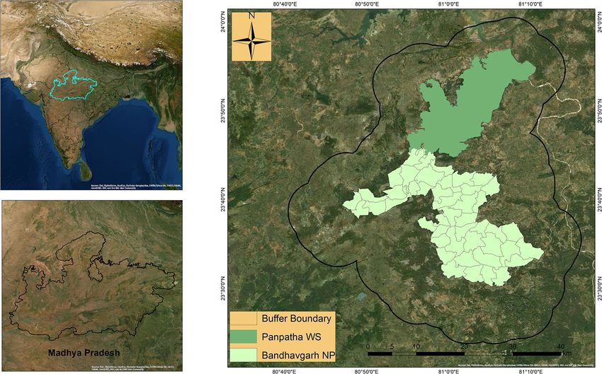
www.nature.com/scientificreports/
six tiger conservation landscapes of global conservation importance occur in the Indian s ubcontinent4. Overall,
these landscapes provide habitat to over 50% of the estimated global population of wild tigers5,6.
In India, most of the tiger population is primarily restricted to the tiger reserves. A tiger reserve consists of
an undisturbed core area wherein human settlements, livestock grazing, and resource utilization are prohibited
under the Wildlife Protection Act, 1972. The core zone is further supplemented by the surrounding multi-use
buffer zones, which act as population sinks. With better and strict conservation policies now employed by Govt.
of India for the conservation of tigers and sympatric co-predators, there is an increased likelihood of tiger popula-
tions increase in the future. Consequent to this increase in the population of large carnivores within the limited
habitats, the human-wildlife conflict in the future may be intense.
The fifth assessment report developed by the Inter-Governmental Panel for climate c hange7 projects the
global surface temperature to exceed 1.5 °C by the end of the twenty-first century relative to 1850–1990 under all
four Representative Concentration Pathway (RCP) scenarios. The report also projects the risk of climate-driven
extinction for a large fraction of species during and beyond the twenty-first century. Climate change poses a
new challenge for biodiversity conservation in the twenty-first century8 because the climate is one of the key
environmental predictor variables of species d istribution9. In response to climate change, species may shift to
new geographically available climatic zones, adapt to new climatic conditions by means of phenotypic plasticity,
or through genetic changes (evolution) or go locally e xtinct10,11. Many mammals across the world have already
shifted their geographic ranges in recent d ecades12,13. Large mammals, particularly apex predators, are more
sensitive to climate change and habitat f ragmentation14.
Estimating the potential changes in the distribution of species under future climatic scenarios is thus impor-
tant, particularly in the disturbed and fragmented landscapes which are more sensitive to the impacts of cli-
mate change. Species in their environment select habitat resources that determine their distribution across the
range of spatial scales. Thus including the predictor variables at inappropriate spatial scale may lead to wrong
conclusions15. It is therefore imperative to correctly identify the spatial scale at which the predictor variables best
determine the distribution of species. Since the distribution of the species depends on the processes occurring at
multiple spatial s cales16–18, multi-scale distribution models can increase the predictive ability of the distribution
models relative to single-scale m odels17. Multi-scale approaches are more informative and offer better insights
into species habitat requirements19–21.
Several robust statistical approaches are available to model the species distribution in relation to the habitat
variables22,23. Recently, however, machine learning algorithms such as Maximum Entropy Modelling (Max-
Ent)24,25, Random f orests26, Classification and Regressions Tress (CART)27 have been shown to outperform
the traditional regression-based approaches. Cushman and W asserman28 used multiple logistic regression and
random forest algorithm in their study of multi-scale habitat selection of American martens (Martes americana).
They found that the random forest outperformed the logistic regression approach. Similar studies of species
distribution modeling report the superior ability of random forest in comparison to traditional regression-based
algorithms29–34.
The traditional regression modelling approaches are strictly assumption based (e.g., normality, data independ-
ency, and additivity) and the predictor variables need to be pre specified. These model assumptions are seldom
true in ecological context. In case of large number of explanatory variables, the traditional regression based
approaches have tendency of overfitting the data unless some information criteria such as Akaiki Information
Criterion (AIC) are employed to reduce the number of parameters. These limitations of conventional modelling
approaches can be easily overcome by using more flexible, non-parametric algorithms such as random forest.
Likewise, the likelihood based modelling approaches such as occupancy models cannot accommodate complex
non-linear effects and interactions between predictor variables or covariates and are thus more suited for describ-
ing linear effects and simple interactions.
In this study, we used a random forest algorithm to investigate the scale-dependent habitat selection of tigers
and leopards in the disturbed and human-dominated landscapes of central India, one of the important tiger
conservation landscape areas of global conservation importance. We used scale optimized variables and predicted
the habitat suitability models for tigers and leopards under the current and future climatic scenarios using the
species occurrence data collected between 2017 and 2018. We used Environmental Niche Models (ENMs) to
evaluate the patterns of niche similarity between tiger and leopard. The ENMs represent the predicted suitability
of species or population in the landscape. These predicted suitabilities can be compared from different popula-
tions or species to test the underlying hypothesis about niche conservation or niche d ivergence35–37. The degree
to which ecological niches between closely related species have been conserved over time has many implications
in ecology and evolution of the species. Though ENMs can be used to compare the predicted environmental
suitabilities between species, the statistical tests for assessing the similarities in the observed overlaps or testing
the hypothesis of niche conservation between species or populations are lacking or conceptually ambiguous37.
Many authors argue that such methodological ambiguity has led to the absence of general conclusions about
niche conservation38–40. Second limitation in the studies comparing the niches of two species or populations stems
from the fact that niche similarity is quantified in geographic space (G-space)37,41 rather than environmental
space (E-space)42,43. The G-space is the geographic distribution of species represented by latitude and longitude
that exists for any given time. The E-space as put by Broennimann et al.42 is defined by axes of chosen analysis
(usually ordination such as PCA) and is bound by the maximum and minimum values of environmental vari-
ables found across the entire regions. Thus E-space may be viewed as the multidimensional space of environ-
mental variables across the geographic space at any particular time, mostly characterized by first two principal
components from principal component analysis44. Most popular methods of using E-space available are those of
Broennimann et al.42 which comprises of two statistical tests. First statistical test called as niche equivalency test
uses a monte-carlo resampling statistic to assess how similar two niches are and second test is a randomization
Scientific Reports | (2020) 10:11473 | https://doi.org/10.1038/s41598-020-68167-z 2
Vol:.(1234567890)
www.nature.com/scientificreports/
Figure 1. (a) Frequency of selected scales (in meters) across the range of predictor variables for assessing the
multi-scale habitat associations of tiger. (b) Frequency of selected scales (in meters) across all predictor variables
used to assess the multi-scale habitat associations of leopard.
test used to assess the power (of the equivalency test) to detect the significant differences in equivalency statistic
and is called background test.
In this study, we use E-space based niche equivalency test statistic introduced by Brown and C arnaval44
based on methods proposed by Broennimann et al.42 and Qiao et al.45 to test for the significant differences in the
environmental niches of tiger and leopard using R package ‘Humboldt’44. We use niche overlap test and niche
divergence test to recognize the differences in environmental niches that emerge from the true niche divergence
instead of other subtle causes such as difference in life history strategies, or simply due to the space limitations
within the habitats44. Niche overlap test or niche equivalency test estimates the degree of similarity between
the occupied niches and niche divergence test or niche background test estimates the portion of the accessible
environment space shared by two species44. The niche overlap test determines how equivalent (or dissimilar) the
occupied niches of two species are given the common environmental space in which they occur and in turn the
niche divergent test determines the significant differences in the environmental space occupied by two species.
The significant value of niche divergence test indicates that the niches of two species sharing common environ-
mental space are not equivalent and thus the fundamental niches have resulted due to the divergent evolution.
Results
Univariate scaling. A total of eight spatial scales (3,500–28,000 m) for each predictor variable except road
and river density were chosen for univariate random forest modeling. Although the scales were selected across
the broad range of variables, the scales at a broader spatial extent (28,000 m) had the highest frequency of selec-
tion in both the predators (Fig. 1a,b).
Scientific Reports | (2020) 10:11473 | https://doi.org/10.1038/s41598-020-68167-z 3
Vol.:(0123456789)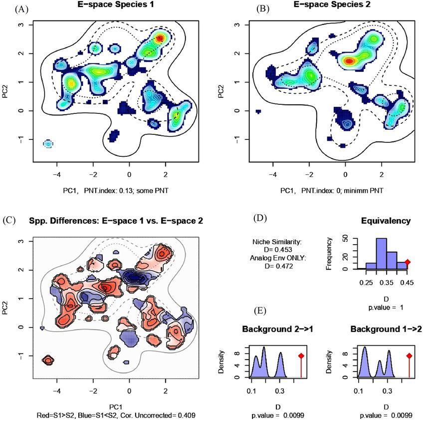
www.nature.com/scientificreports/

                                      Figure 2.  (a) Model improvement ratio (MIR) plot for the selected variables used in the final multiscale
                                      habitat model of tiger. Sal dominated forests at the spatial scale of 28,000 m was the most important predictor
                                      variable and road density within the focal radius of 4 km was the least important variable. The other variables
                                      are listed in order of their importance relative to sal dominated forests, with the x-axis indicating the relative
                                      additional model improvement when adding each successive variable. (b) Model improvement ratio (MIR) plot
                                      for the selected variables used in the multiscale habitat model of leopard. Sal mix forest at the spatial scale of
                                      21,000 m was the most important predictor variable and aspect within the focal radius of 28,000 m was the least
                                      important variable. The other variables are listed in order of their importance relative to sal mix forest with the
                                      x-axis indicating the relative additional model improvement when adding each successive variable.

                                      Multivariate modeling. A total of 13 and 10 variables based on model improvement ratio plots (MIR)
                                      were retained in the final multivariate models of tiger and leopard (Fig. 2a,b). In the case of tigers, four variables
                                      (sal dominated forests, scrub habitats, sal mix forests and bio17) were selected at the broadest scale (28,000 m).
                                      Three variables (aspect, human population density and degraded forest patches) were selected at a small spatial
                                      scale (3,500 m), and four variables were selected at intermediate spatial scales (Human settlements, farmlands,
                                      bio14 and slope) (7,000–17,500 m). The road density was used at two spatial scales (1,000 and 4,000 m) (Fig. 2a).
                                      In the case of leopards, seven variables (sal mix forests, human settlements, scrub habitat patches, degraded
                                      forests, agriculture, bio17 and aspect) were selected at broadest scales (21,000–28,000 m) (Fig. 2b). Three of the
                                      variables (slope, moist deciduous forests and farmlands) were selected at intermediate scales (10,000–14,000 m).

                                      Variable importance and partial dependency plots of tiger.                  The percentage of sal dominated forests
                                      at the broadest spatial scale (28,000 m) was the most important predictor variable based on MIR plots (Fig. 2a).
                                      Tiger occurrence showed a decreasing relationship with the increasing percentage of sal dominated forests at the
                                      broadest scale (Fig. 3a). Aspect at the spatial scale of 3,500 m was the second important variable (Fig. 2a). Tigers
                                      showed a strong unimodal association with the south-facing slopes (Fig. 3b). Tigers responded to the human
                                      settlements, and human population density at small spatial scales (7,000 m and 3,500 m) with the highest pre-
                                      dicted occurrences at a lower percentage of settlements and lower human population density (Fig. 3c,d). Among
                                      bioclimatic variables, only precipitation of driest month (Bio14) and precipitation of driest quarter (Bio17) were
                                      retained as important variables in the multivariate random forest model (Fig. 2a). Tigers responded to bio14 at
                                      a small spatial scale and showed the highest predicted occurrences at higher values of the precipitation (Fig. 3b).
                                          In contrast, bio17 was most influencing at the broadest scale. The highest occurrences of tigers were predicted
                                      at the intermediate levels of precipitation in the driest quarter (Fig. 3b). The mosaic of croplands and natural

          Scientific Reports |   (2020) 10:11473 |               https://doi.org/10.1038/s41598-020-68167-z                                               4

Vol:.(1234567890)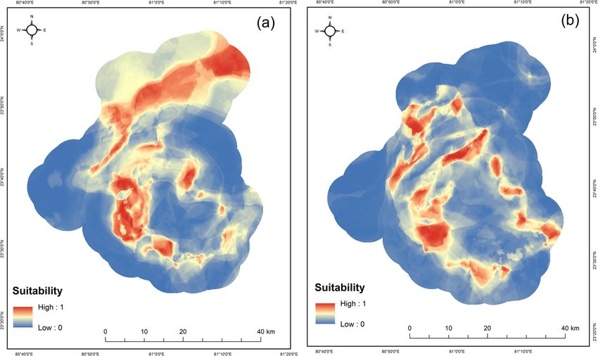
www.nature.com/scientificreports/

                            Figure 3.  (a) Partial dependency plots showing the marginal effect of degraded forests, sal dominated forests,
                            sal mix forests and scrub patches on the predicted occurrence of tiger. (b) Partial dependency plots showing
                            the marginal effect of bio14, bio17, farmland and aspect on the predicted occurrence of tiger. (c) Partial
                            dependency plots showing the marginal effect of slope, human population density and road density on the
                            predicted occurrence of tiger. (d) Partial dependency plot showing the marginal effect of human settlement on
                            the predicted occurrence of tiger.

                            vegetation was most influencing at a small spatial scale of 7,000 m. Tigers showed the tendency to avoid the
                            habitats with a higher percentage of farmlands (Fig. 3b). Tigers responded to the open scrub habitats at the lower
                            percentage and broadest scale (28,000 m). Tigers chose very gentle slopes at the intermediate scale (17,500 m)
                            with a strong unimodal relationship around 2 degrees of steepness (Fig. 3c). Tigers showed a strong unimodal
                            preference for sal mixed forest at the broadest spatial scale (Fig. 3a). The degraded forest patches were perceived
                            at small spatial scales and tigers showed an overall avoidance of degraded forests (Fig. 3a). There was a strong
                            unimodal relationship between tigers and road density within 1 km, and the highest occurrences of tigers were
                            predicted at 0.2 densities of roads within 1 km focal radii (Fig. 3c). In contrast, we observed a moderate relation-
                            ship relative to the road density within 4 km focal radii (Fig. 3c).

                            Variable importance and partial dependency plots of leopard.                      Leopards showed a preference for
                            the high percentage of sal mix forests at a broader spatial scale (Fig. 4a). Leopards showed a unimodal preference
                            for moist deciduous forests at medium concentrations and intermediate spatial scale (Fig. 4a). Leopards pre-
                            ferred the mosaic of cropland and natural vegetation at an intermediate spatial scale (10,500 m) with the highest
                            occurrence predicted at a lower percentage of farmland (Fig. 4a). High preference of leopard for the intermedi-
                            ate percentage of degraded habitats occurred at a broader spatial scale (Fig. 4b). A strong unimodal relationship
                            existed between leopards and the percentage of agricultural patches at a broader spatial scale (Fig. 4b). The
                            precipitation of driest quarter (bio17) had a unimodal effect on the habitat selection of leopards best explained at
                            the broadest spatial scale (Fig. 4b). The aspect was the tenth important predictor variables influencing the habitat
                            selection of leopards at the broadest spatial scale (28,000 m) with a high occurrence of leopards along southern
                            slopes (Fig. 4b). A unimodal relationship was predicted at a lower percentage of human settlements at a broader
                            spatial scale (Fig. 4c). Leopards showed a general preference for gentle slopes with the highest predicted occur-
                            rence at 2.5° (Fig. 4c).

                            Distribution of tigers and leopards under current and future climatic scenarios. The spatial dis-
                            tribution of tigers and leopards was predicted using the scale optimized predictor variables selected in the pro-

Scientific Reports |   (2020) 10:11473 |               https://doi.org/10.1038/s41598-020-68167-z                                             5

                                                                                                                                         Vol.:(0123456789)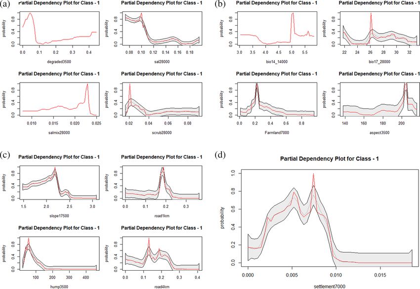
www.nature.com/scientificreports/

                                      Figure 4.  (a) Partial dependency plot showing the marginal effects of farmland, moist deciduous forests, sal
                                      mix forests and scrub habitats on the predicted occurrence of leopard. (b) Partial dependency plot showing
                                      the marginal effect of agriculture, aspect, bio17, and degraded forests on the predicted occurrence of leopard.
                                      (c) Partial dependency plots showing the marginal effect of human settlements and slope on the predicted
                                      occurrences of leopard.

                                      cess of variable importance in multiscale random forest models. The accuracy for the distribution maps of leop-
                                      ards was discriminately high (AUC = 0.90, TSS = 0.80) in comparison to tigers (AUC = 0.83, TSS = 0.66). A total
                                      of 65,499.17 (42.64%) and 39,770.20 (25.89%) hectares of suitable habitat exists for tigers and leopards under the
                                      current climatic scenario. The suitable area for tigers included the northern Panpatha wildlife sanctuary, which
                                      forms the core zone of the reserve and the dense sal dominated forest in the southeastern parts of the reserve
                                      (Fig. 5). For leopards, the most suitable areas included the forested areas at the edges of the core-buffer bound-
                                      ary of the reserve (Fig. 5). We predicted the change in the distribution of tigers and leopards under the most
                                      conservative emission pathway scenario (RCP 2.6) and worst emission scenario (RCP 8.5). Our model showed
                                      the overall loss in the suitable habitat of tigers under both the scenarios, while our model predicted overall gain

          Scientific Reports |   (2020) 10:11473 |               https://doi.org/10.1038/s41598-020-68167-z                                             6

Vol:.(1234567890)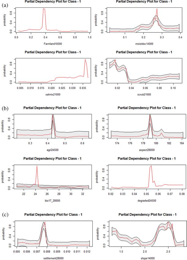
www.nature.com/scientificreports/
Figure 5. Predicted habitat suitability under current climatic scenario based on the scale optimized predictor
variables using Random forest algorithm. Panel (a) represents the habitat suitability of tiger and panel (b)
represents the suitability of leopard. Red color denotes high suitability and blue color indicates low suitability.
in habitats for leopards (Fig. 6). The highest loss (23%) in the suitable habitat of tigers was predicted under RCP
8.5 for the years the 2050s and 11% under RCP 2.6 for the years 2050s (Table 1).
The highest gain (11.41%) in the suitable habitat was also predicted under RCP 8.5 for the 2050s. The gain
in suitable habitat was more pronounced relative to the loss in the habitat for leopards under both the emission
scenarios (Table 1). The highest gain in habitat was predicted under RCP 8.5 (18.12%), followed by RCP 2.6
(17.15%). The amount of the habitat loss was predicted to be almost the same for leopards under all pathway
scenarios.
Niche similarity between tiger and leopard. The PCA analysis revealed that 71.9% of the variance
(PC1 = 52.5% and PC2 = 19.4%) in environmental data input can be represented in a 2 dimensional E-space
(Fig. 7). The dimension with the most explained variance is plotted on horizontal axis of the PCA correlation
circle and second most explanatory variables are plotted on vertical axis of the PCA plot (Fig. 7). We obtained
a non-significant niche equivalency test statistic (D = 0.45, p = 1) indicating identical environmental niches of
tiger and leopard and a significant background test statistic (p = 0.009) (Fig. 8). The significant background test
statistic indicates tiger and leopard are more similar than expected by chance. The Potential Niche Truncation
Index (PNTI) for tiger and leopard (Fig. 8) falls well below the proposed range of the values associated with
either moderate risk (0.15–0.3) or high risks (0.3) that observed niches do not represent the fundamental niches.
Thus the observed niches of tiger and leopard represent the fundamental niches of these species.
Discussion
Machine learning algorithms are relatively more flexible, accurate, and often require less time than traditional
approaches. When using random forest, there is no limitation on the number of predictor variables used com-
pared to the traditional approaches. More traditional approaches such as general linear models, and occupancy
approaches depend on technical expertise to meet statistical assumptions to produce the unbiased output. How-
ever, more accurate distribution maps of the species are needed for the sustainable management of globally
threatened species which can be produced using machine learning algorithms. In this study, we explore the
applicability of random forest for building multi-scale distribution maps for tiger and leopard in the human-
dominated landscapes of central India. In this study we focused on three important components of the spatial
ecology of tigers and leopards: the use of multiple spatial scales in assessing the species habitat relationships,
using scale optimized predictor variables to predict the HSMs of tigers and leopards under current and future
climatic scenarios and finally determining the patterns of niche conservatism between tigers and leopards. Each
of these components is briefly discussed below.
Scale‑dependent habitat selection of tiger and leopard. The scale-dependent habitat relationships
among carnivore species have been shown to outperform the approaches of single scale habitat association
studies46–48. In our multiscale habitat selection study, both the predators responded to most of the habitat vari-
ables at broader spatial scales, which are in general agreement with similar studies of other carnivore species at
Scientific Reports | (2020) 10:11473 | https://doi.org/10.1038/s41598-020-68167-z 7
Vol.:(0123456789)
www.nature.com/scientificreports/
Figure 6. Predicted change in the distribution of tigers and leopards under future climatic scenarios. Panels
(a) and (b) represent the change in distribution of tiger under RCP 2.6 scenario for the years 2050s and 2070s.
Panels (c) and (d) represent the change in distribution of tiger under RCP 8.5 for the years 2050s and 2070s.
Panels (e) and (f) represent the change in the distribution of leopard under RCP 2.6 Scenario for the years 2050s
and 2070s and panels (g) and (h) represent the predicted change in the distribution of leopard under RCP 8.5
for the years 2050s and 2070s. The map was created using ArcGIS (v 10.3) software developed by ESRI. https://
www.esri.com.
Total suitable Stable habitat Stable habitat Net gain/net loss Net gain/net
Species Scenario habitat (ha) (%) Gain (ha) Gain (%) Loss (ha) Loss (%) (ha) loss (%)
Current 65,499.17 65,499.17 100.00
RCP 2.6 (2050) 64,987.03 58,125.97 88.74 6,861.06 10.48 7,373.20 11.26 − 512.14 0.0013
Tiger RCP 8.5 (2050) 57,764.33 50,289.49 76.78 7,474.84 11.41 15,209.68 23.22 − 7,734.84 − 0.0012
RCP 2.6 (2070) 64,377.20 61,732.99 94.25 2,644.20 4.04 3,766.18 5.75 − 1,121.97 − 0.0001
RCP 8.5 (2070) 61,701.48 60,226.52 91.95 1,474.95 2.25 5,272.65 8.05 − 3,797.69 − 0.0004
Current 39,770.19 39,770.19 100
RCP 2.6 (2050) 43,564.73 36,745.43 92.39 6,819.30 17.14 3,024.76 7.60 3,794.54 0.0009
Leopard RCP 8.5 (2050) 44,120.20 36,914.83 92.82 7,205.37 18.11 2,855.36 7.17 4,350.01 0.00012
RCP 2.6 (2070) 42,152.81 36,730.46 92.35 5,422.34 13.63 3,039.73 7.64 2,382.62 − 0.0004
RCP 8.5 (2070) 42,585.37 37,201.631 93.54 5,383.74 13.53 2,568.56 6.45 2,815.18 0.0001
Table 1. Predicted change in the distribution of tigers and leopards in and around Bandhavgarh Tiger
Reserve, Madhya Pradesh, India under low (RCP 2.6) and high (RCP 8.5) Representative Concentration
Pathway scenarios for the timeline 2050s and 2070s using the model developed by Model for Inter-disciplinary
Research on Climate change (MIROC5).
multiple spatial scales. Khosravi et al.47 found a strong association of three sympatric carnivores relative to habi-
tat variables at broader spatial scales. Cushman and W assermann28 found American martens responded strongly
to predictor variables at broader spatial scales. Our study confirms the findings of the previous studies that large
carnivores respond to habitat variables at broader spatial scales.
Scientific Reports | (2020) 10:11473 | https://doi.org/10.1038/s41598-020-68167-z 8
Vol:.(1234567890)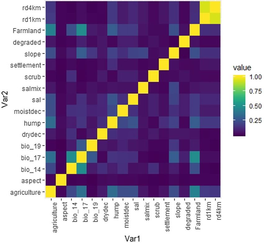
www.nature.com/scientificreports/
Figure 7. Niches of tiger and leopard in two dimensional E-space. Panels (A) and (B) represent the niches of
species along first two axes of the PCA. The species occurrences are represented by kernel density isopleths,
red color indicates high density and cooler color (blue) indicates low density. Solid and dotted contour lines
illustrate 100% and 50% of the available background (environmental space). Panel (C) represents the difference
in the E-space of two species and Niche E-space Correlation Index (NECI). NCEI determines if one should
correct the occurrence densities of each species by the prevalence of their environments in their range for
equivalency and background tests. For high NCEI (> 0.5) species occupied niches are recommended to be
corrected by the frequency of E-space in accessible environments to reduce the chances of committing type 1
errors, and panel (D) represents the correlation circle and important principal components of the raw input
data.
The relationships between tiger occurrences and human-influenced variables at a small scale reflect the ten-
dency of tigers to avoid anthropogenic pressure in disturbed and human-dominated landscapes at a fine-scale,
indicating tigers prefer undisturbed habitats within their immediate vicinities. The broad-scale relationship
between sal and sal mix forests and tiger occurrences indicates the importance of dense forest cover for the
daily movement and dispersal of tigers at broader scales. Tigers are ambush hunters and cover large distances
in search of suitable prey48; thus, they need dense forest cover to avoid early detection by prey species49. The
dense forests of sal and sal associated species may provide ample cover to tigers while covering large distances at
broader spatial scales. In contrast, leopards showed relationships with human-influenced variables at broader and
medium spatial scales which points towards their broader plasticity or adaptability to anthropogenic factors in
human-dominated landscapes at a broader scale. The association of leopards with the habitats at the core-buffer
interface reflects the tendency of leopards to occupy edges that represent the high human-use zones.
Our study indicates that habitat specialist species such as tigers tend to occur in less disturbed habitats with
thick vegetation cover and need continuous tracts of connected forests at broader spatial scales. The habitat
generalist species like leopards due to their broader plasticity and adaptability tend to occur in e dges50–52 with
avoidance of human disturbances at a broader spatial scale.
Scientific Reports | (2020) 10:11473 | https://doi.org/10.1038/s41598-020-68167-z 9
Vol.:(0123456789)www.nature.com/scientificreports/
Figure 8. Niche equivalency and niche background tests between tiger and leopard. Panels (A) and (B)
represent the kernel density isopleths, red color indicates high density and cooler color (blue) indicates low
density. Panels (A) and (B) also represent the Potential Niche Truncation (PNT) Index describing the amount of
observed E-space of the species that is truncated by the available E-space. Panel (C) represents the difference in
the E-space of two species and Niche E-space Correlation Index. Panel (D) represents the Equivalency statistic
measured as Niche similarity index and panel (E) represents niche Background statistic.
Habitat suitability of tigers and leopards under current and future climatic scenarios. In this
study, we predicted the suitability of the tiger and leopard relative to scale optimized predictor variables using
the random forest algorithm. The predicted suitability maps of tigers and leopards show suitable areas for tigers
in dense forests with less human interference and leopards occupied the edges at the core-buffer interface of the
reserve (Fig. 5). The dense forests are associated with high prey densities in comparison to disturbed habitats.
Chita, sambar and wild pig are some of the most important prey species generally associated with undisturbed
habitats and occur more frequently in the diet of t igers48,53. Sambar, one of the important prey species, is known
to avoid disturbed areas54,55 actively. Tigers are ambush hunters and cover large distances in search of suitable
prey48 thus require dense forest cover to avoid early detection by prey species56. The dense sal and sal mix forests
may provide ample cover to tigers while covering large distances at broader spatial scales. Thus habitat specialist
species such as tigers tend to occur in less disturbed habitats with thick vegetation cover and need continuous
tracts of connected forests at broader spatial scales. In contrast, leopards showed high occurrences within dis-
turbed habitats at the core-buffer interface of the reserve reflecting their tendency to occupy edges representing
high human-use zones. The habitat generalist species like leopards due to their adaptability tend to occur in the
edges57,58 with high tolerance to the presence of humans51,52.
We observed considerable loss of suitable habitat for tigers under all emission scenarios and overall gain in
case of leopard (Table 1). Tigers are habitat specialists preferring the areas with dense vegetation cover, high prey
Scientific Reports | (2020) 10:11473 | https://doi.org/10.1038/s41598-020-68167-z 10
Vol:.(1234567890)www.nature.com/scientificreports/
density, and less human footprint59. Different species are reported to respond to the impacts of climate change
differently60. Pandey and Papeş61 reported expansion in the habitats of generalist mammalian species under future
climatic scenarios. Leopards by their broader niches and ecological plasticity, may cope and adapt to the impacts
of future climatic changes better than tigers. Our study agrees with the findings of Tian et al.62, who predicted
that Amur tigers (Panthera tigris altaica) would go extinct fastest in severe climate change scenarios. Some
authors argue that leopards due to their globally broad distribution can remain unaffected or even benefit from
the impacts of climate change as long as their potential prey species suffice63. Our study also predicts the highest
loss in the potential habitat of tigers under high emission scenarios (RCP 8.5) and expansion in the habitats of
leopards under all emission scenarios. Despite the successful application of climatic models to predict the change
in the distribution of wide range of species at large scales, they have been questioned for lacking the details on
species interactions and species dispersal capabilities. For example, tiger densities are directly dependent on
prey abundances64 and thus, the change in the distribution of tigers may also depend on how the prey species
would respond to the future climate change. Tigers have great dispersal abilities; however the persistent habitat
fragmentation and isolation between the protected areas may negatively affect their populations. Thus in future,
the increased inter-patch connectivity and maintaining prey species at high densities may locally increase the
tiger sub-populations.
Environmental niche overlap between tiger and leopard. Although we focused on two measures of
niche overlap between tiger and leopard in this study, there are other alternatives which may be better suited for
particular studies. We observed moderate niche similarity between tiger and leopard (D = 0.54). The non-signif-
icant niche similarity test statistic and significant background test statistic suggest a degree of niche conservation
between tiger and leopard. We stress here that in this analysis we have treated niche conservation as the ten-
dency of closely related species to share similar traits. However, despite having somewhat similar environmental
niches, tigers and leopards varied in their use of specific environmental resources. For example, the ENMs of
tiger and leopard showed that tigers occupied dense sal forests with a low human footprint while as suitable
areas for leopards included habitats at core-buffer interface with a high human footprint. Leopards tend to avoid
tigers when they co-occur and thus use buffer zones around protected areas in India51. Similar results of leopards
avoiding tigers spatially are regarded as a mechanism of spatial segregation between them65–67. In this study, we
assessed the environmental niche overlap between the tiger and leopard along the only spatial dimension. How-
ever, the carnivore communities are shaped by complex, competitive interactions. High niche similarity among
the competing species in one niche dimension is followed by niche dissimilarity in other niche dimensions68,69.
Sympatric carnivores may achieve the ecological coexistence by using different habitats70–72 selecting different
prey sizes62 or have non-overlapping activity patterns70–72.
Conclusion and management implications. Our study highlights three key components concerning
the spatial ecology of two large carnivores in human-dominated landscapes. Our study shows how two ecologi-
cally similar species differ in their use of habitat resources across spatial scales. While tigers perceive human
avoidance at a small scale, leopards respond to human interference at a broader scale indicating the low tolerance
level in tigers towards humans than leopards. The results of multi-scale HSMs of tigers and leopards indicate
the importance of dense forest habitats at a broader scale. The regional and landscape planning to mitigate the
impacts of future climate change on the persistence of tigers is thus needed. Increasing the forest cover and
inter-patch connectivity by building corridors and maintaining prey species at high densities are particularly
important management and conservation strategies that could be undertaken for the persistence of tigers.
Materials and methods
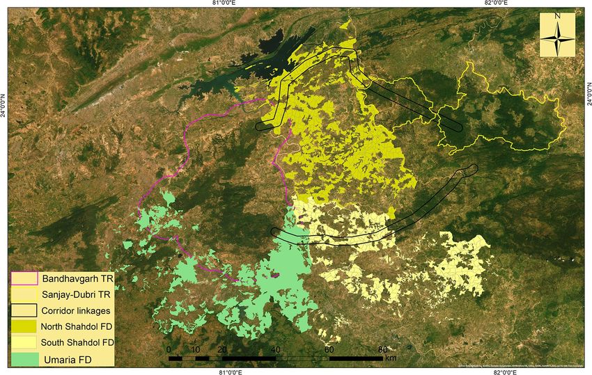
Study area. Bandhavgarh Tiger Reserve (BTR) is located between 23° 27′ 00″ to 23° 59′ 50″ North lati-
tude and 80° 47′ 75″ to 81° 15′ 45″ East longitude in the Umaria district of Madhya Pradesh, in central India
(Fig. 9). The core zone of the reserve includes the Panpatha Wildlife Sanctuary (PWS) in north and Bandhavgarh
National Park (BNP) in the south, together with having an area of 716 km2. The surrounding buffer zone has an
area of 820 km2, adding the total area of the reserve to 1536 km2. The reserve is surrounded by the fragmented
and human-dominated territorial forest ranges of the North Shahdol Forest Division (NSFD) in the north and
northeast and south Shahdol Forest Division (SSFD) in the south-southeast. The territorial forest division of dis-
trict Umaria (UFD) surround the reserve in extreme south and southwest, and the Katni forest division (KFD)
is located to the west of the reserve. The Sanjay-Dubri Tiger Reserve (SDTR) and Guru-Ghasidas Tiger Reserve
(GGTR) are located about 80–150 km from the BTR in the northeast and southeast, respectively. The whole
landscape (BTR, SDTR, NSFD, SSFD, and GGTR) is regarded as an important tiger and elephant conservation
unit (Fig. 10).
BTR represents the moist deciduous vegetation dominated by sal (Shorea robusta) and sal mixed forests. The
overall vegetation of the BTR comprises moist peninsular low-level sal forest, northern dry mixed deciduous
forest, dry deciduous scrub, dry grassland and west Gangetic moist mixed deciduous forest73. BTR supports a
wide variety of faunal assemblages from small invertebrates to the largest bovid in Asia. There are 35 mammalian
species, over 250 species of birds, and a wide variety of butterflies in reserve. The deer species include chital
(Axis axis), sambar (Rusa unicolor) and barking deer (Muntiacus munjtak). Indian gazelle (Gazella bennetti),
four-horned antelope (Tetracerus quadricornis) and Indian blue bull (Boselaphus tragocamelus) are the three
antelope species in BTR. Northern plains gray langur (Semnopithecus entellus) and rhesus macaque (Macaca
mulatta) represent the two primate species, and the suidae family is represented by a wild pig (Sus scrofa). The
reserve also holds a good population of re-introduced gaur (Bos gaurus).
Scientific Reports | (2020) 10:11473 | https://doi.org/10.1038/s41598-020-68167-z 11
Vol.:(0123456789)www.nature.com/scientificreports/
Figure 9. Location of the Bandhavgarh Tiger Reserve, Madhya Pradesh, India. Map of the study area was
created using ArcGIS (v 10.3) software developed by ESRI. https://www.esri.com.
Figure 10. Map showing the Bandhavgarh Tiger Reserve (BTR), Sanjay-Dubri Tiger Reserve (SDTR) in the
west, North Shahdol Forest Division (NSFD), South Shahdol Forest Division (SSFD), between BTR and SDTR
and Umaria Forest Division (UFD) in south and south east of BTR. The map was created using ArcGIS (v 10.3)
software developed by ESRI. https://www.esri.com.
Scientific Reports | (2020) 10:11473 | https://doi.org/10.1038/s41598-020-68167-z 12
Vol:.(1234567890)www.nature.com/scientificreports/
Major large carnivore species include tiger (Panthera tigris), leopard (Panthera pardus), sloth bear (Melur-
sus ursinus), Indian wolf (Canis lupus), Asiatic wild dogs (Cuon alpinus) and striped hyena (Hyaena hyaena).
Golden jackal (Canis aureus), Indian fox (Vulpes bengalensis), jungle cat (Felis chaus), Asiatic wildcat (Felis lybica
ornata), rusty-spotted cat (Prionailurus rubiginosus) and fishing cat (Prionailurus viverrinus) are the medium-
sized carnivores in reserve.
Species occurrence data and spatial auto‑correlation. The species occurrence data was obtained by
collecting the scats of tigers and leopards in the study area. We collected 381 and 343 scats of tigers and leopards
between 2017 and 2018. The identification of the scats was based on secondary evidence such as diameter range,
and presence of associated ancillary signs like tracks74,75. Andheria et al.76 confirmed the accuracy of scat identi-
fication using the same features with fecal DNA tests. The scats where the identity of the predator was ambigu-
ous were not collected. We obtained an additional 95 and 74 camera trap detection of tigers and leopards in a
camera trap survey in the buffer zone of the reserve. We implemented spatial filtering using the SDM t oolbox77
in ArcGIS (10.3) to reduce the inherent spatial bias in the species presence records. The scats and camera trap
photo-captures of tigers and leopards were spatiality rarified at the distance of 1,000 m from each other. Lacking
the real absence points, we randomly generated pseudo-absence points in ArcGIS (10.3) in an approximately
equal number to the original occurrence points of the tiger and leopard to deal with the problems arising from
unbalanced prevalence78. This was achieved by first generating 500 random pseudo absence points and then
discarding the absence points within the buffer radius of 500 m of the original occurrence points of tiger and
leopards to reduce the number of false negatives79. The buffer distance can be either set arbitrary or based on
species attributes80. Out of 476 and 417 occurrence records for tigers and leopards, we retained a total of 184 and
261 spatially rarified occurrence locations and an equal number of pseudo absence points of tigers and leopards
for final random forest modeling.
Environmental predictors. A total of 40 environmental predictor variables (Table 2) were used in pre-
dicting the species habitat relationships. We grouped predictor variables into five broad categories as climatic,
topographic, landscape composition, vegetation, and human-influenced.
These predictor variables were selected based on the similar habitat relationship studies of large carnivores.
We obtained the bioclimatic variables from the WORLDCLIM database (https: //www.worldc lim.org). We tested
the correlation among predictor variables at (|r| > 0.50) and subsequently removed the highly correlated vari-
ables using R packages “rfUtilities” and “randomForest”81 implemented in R 82 to account for multi-colinearity
among predictor variables83 as multi-colinearity may alter the model predictions to the significant extent84. The
package “rfUtilities” removes the redundant variables using qr matrix decomposition (0.05 threshold) and thus
only the least correlated variables (|r| < 0.50) were retained for further modelling (Fig. 11). We obtained a digital
elevation map of the study area from the Shuttle Radar Topography Mission (SRTM) elevation d atabase85,86.
Slope, aspect, topographic ruggedness index was derived from the elevation layer using surface analysis tools
in the Spatial Analyst toolbox in ArcGIS (10.3). We obtained the land use land cover (LULC) from the Indian
Institute of Remote Sensing (IIRS, https: //iirs.gov.in). The LULC layer included nine land use categories as dense
sal dominated forests, sal mix forests, moist deciduous forests, dry deciduous forests, scrub habitats, grasslands,
agriculture, water bodies and permanent human settlements. We calculated seven topographic variables includ-
ing elevation, slope, aspect, topographic roughness, road density and river density. We calculated road and river
density using the line density tool in ArcGIS at the spatial scale of 1,000, 2,000, 3,000 m. We used road and
river density instead of Euclidean distance because of the high concentration of roads in the buffer zone of the
reserve. Thus we used the percentage of roads and rivers within the radius 1,000, 2,000, and 3,000 m of the specie
presence-absence. Monthly Normalized Difference Vegetation Index (NDVI) version 6 (MOD13Q1) generated
every 16 days available at the spatial resolution of 250 m was obtained from the MODIS website (https://lpdaa
c.usgs.gov/products/mod13q1v006/). We reclassified the 23 NDVI layers into three seasons corresponding to
summer, wet, and winter seasons. We resampled all the variables at the spatial resolution of 90 m using the SDM
toolbox in ArcGIS (10.3).
Future climatic data. At present, climatic models are the best tools for simulating future climatic
scenarios88. However, the variations within and among the different climatic models may pose problems in iden-
tifying the most robust and optimal model to use88. Though, no clear guidance on how and which climatic mod-
els to select exists, and researchers have little objectivity in selecting the climatic models87. The final decision may
sometimes be influenced by the assumption (though not always correct) that a climatic model developed in a
particular country will be more robust in that r egion87. In this study, we modeled the change in the potential dis-
tribution of tigers and leopards under two Representative Concentration Pathway Scenarios (RCP 2.6 and RCP
8.5) developed by the Japanese research community called Model for Inter-disciplinary Research on Climate
change (MIROC5)89. These scenarios project the global greenhouse gas emissions based on the assumptions for
a wide range of variables such as human population size, global energy consumption, and change in land-use
patterns. We downloaded Global Climate Models (GCMs) from the WordClim website (https://www.worldclim.
org/cmip5_30s). We aimed to predict the change in the distribution under the most conservative emissions
scenario (closely corresponding to the current rate of greenhouse gas emissions) and the most severe emission
scenarios. The climatic models used in this study represent two extreme scenarios of greenhouse gas emissions.
The RCP 2.6 assumes that global C O2 emissions would peak around 2020 and then fall to values around zero by
2080 and RCP 8.5 is regarded as the worst climatic scenario with higher predicted greenhouse gas emissions.
RCP 8.5 assumes that the global C O2 emissions would increase at a higher rate during the first half of the century
and stabilize by 2100; the concentrations are however three times those in 2 00090–93.
Scientific Reports | (2020) 10:11473 | https://doi.org/10.1038/s41598-020-68167-z 13
Vol.:(0123456789)www.nature.com/scientificreports/
Variable Type Variable Best scale (tiger) Best scale (leopard)
Elevation 24,500 24,500
Slope 17,500 14,000
Topographic Aspect 3,500 28,000
Terrain roughness 24,500 17,500
River density 1,000, 2,000, 3,000 1,000, 2,000, 3,000
Bio1 28,000 24,500
Bio2 28,000 24,500
Bio3 17,500 24,500
Bio4 7,000 21,000
Bio5 21,000 7,000
Bio6 21,000 14,000
Bio7 21,000 7,000
Bio8 28,000 24,500
Bio9 28,000 24,500
Bio10 28,000 28,000
Bio11 14,000 21,000
Climatic
Bio12 7,000 24,500
Bio13 7,000 3,500
Bio14 14,000 10,500
Bio15 28,000 28,000
Bio16 7,000 28,000
Bio17 28,000 28,000
Bio18 24,500 7,000
Bio19 17,500 17,500
Actual evapotranspiration (summer) 10,500 NA
Actual evapotranspiration (monsoon) 17,500 NA
Actual evapotranspiration (winter) NA NA
Sal dominated 28,000 21,000
Sal mix 28,000 21,000
Dry deciduous 24,500 28,000
Landscape composition
Moist deciduous 28,000 14,000
Degraded 3,500 24,500
Scrub 28,000 21,000
NDVI (summer) 7,000 14,000
Vegetation cover NDVI (winter) 21,000 17,500
NDVI (monsoon) 28,000 10,500
Human settlements 7,000 28,000
Human population density 3,500 21,000
Human influenced
Road density 1,000, 3,000, 4,000 1,000, 3,000, 4,000
Farmlands (croplands) 7,000 10,500
Table 2. The set of 40 predictor variables used in the multi-scale habitat modelling of tiger and leopard. First
and second columns represent the type and the name of the variables, and third and fourth columns represent
scale at which each predictor best explained the occurrence of tiger and leopard respectively. Predictor
variables are classified in five groups (Topographic, climatic, landscape composition, vegetation and human
influenced). Road and river density were calculated at four different spatial scales (1, 2, 3, 4 km). Actual
evapotranspiration were not used in the models of leopard and in case of tiger, actual evapotranspiration in
winter season was not used.
Multi‑scale data processing. We calculated the focal mean of each predictor variable across eight spatial
scales (3,500–28,000 m) surrounding each species occurrence location (presence/pseudo absence) using a mov-
ing window analysis with the focal statistic tool in ArcGIS (10.3). Each spatial scale ranging from 3,500 m to
28,000 m surrounding each location was used as search radii for calculating the focal mean of all the predictor
variables expect road and river density. The output of the focal statistics was the raster layers of each predictor
variable at eight spatial scales and .dbf file of extracted raster values around each location of tigers and leopards.
Scale selection and univariate random forest models. The best predictive scale in multi-scale mod-
eling approaches is usually selected by measuring potential environmental predictor variables within different
Scientific Reports | (2020) 10:11473 | https://doi.org/10.1038/s41598-020-68167-z 14
Vol:.(1234567890)www.nature.com/scientificreports/
Figure 11. Multi-colinearity among the predictor variables used in the final random forest modelling of tiger
and leopard. The multi-colinearity was tested at (r > 0.50) using the R package “rfUtilities” and correlogram
was produced using the R package “ENMTools”. The road density is represented at two spatial scales (1 km and
4 km) as shown in the top right corner of the correlogram as rd1km and rd4km, and moistdec, drydec represent
the moist and dry deciduous forests respectively and hump denotes the human population density defined as the
number of persons per square km.
buffer sizes (scales) around species locations (presence/absence) and then to regress each predictor variable
against the response for each scale94,95. Following McGarigal et al.96 and Cushman et al.34, we ran a series of
univariate random forest models for each predictor variable across eight spatial scales (3,500–28,000 m) to select
the appropriate scale at which the predictor variable best explained the probability of species occurrence. The
univariate random forest models were run with the underlying assumption that best fit identifies the most pre-
dictive, and therefore, the single most meaningful, spatial scale across all predictor v ariables15.
Random forest constructs a regression or classification tree by successively splitting the data based on single
predictors. Each split forms a branch in the decision tree and trees are grown without pruning. Random forest
utilizes bagging (bootstrap aggregation) that builds a large number of tress and the model output is obtained by
averaging the aggregated tress or by maximum vote. During bagging, a bootstrap sample is randomly drawn to
build each tree and the data not included in the bootstrap sample is termed as ‘out-of-bag’ (OOB) which is used
to estimate an unbiased error rate and to rank variable importance. We used OOB rates as a measure of selecting
the best predictive spatial scale. In the calculation of OOB error rates, a training data set is created by sampling
with replacement from two-third of the data for each classification tree in a random forest. Each tree is then
used to predict the remaining one-third (‘out of bag’ or ‘bootstrap sample’) of the data. Finally, the OOB error is
computed as the proportion of times that the predicted class is not the same as the true c lass26,81. The scale with
the minimum OOB error rates was selected as the best spatial scale of the predictor variables.
Multi‑scale random forest modeling. Multi-scale random forest models were created using the scale
optimized predictors of tigers and leopards with R package ‘randomForest’81 implemented in R82. Model
Improvement Ratio (MIR) was used to identify the most parsimonious random forest model. In the model selec-
tion process using MIR, the variables were subset using 0.10 increments of MIR values, and all variables above
this threshold were retained for each model. This subset was always performed on the original model’s variable
importance to avoid overfitting. Comparisons were made between each subset model, and the model with the
lowest OOB error rate and lowest maximum within-class error was selected as the final model.
Random forest variable selection. There are several variable selection procedures available in random
f orest97–99 we followed the approach of variable selection developed by Genuer et al.99. This approach is based on
the un-scaled permutation importance that is calculated by permuting each predictor in turn and using the dif-
ference in prediction error (OOB error) before and after permutation as a measure of variable i mportance15,81,100.
This approach is a stepwise procedure whereby a sequence of RF models is estimated by iteratively eliminating or
adding variables according to their importance measures (such as MIR)101. The MIR shows variable importance
measured as the increased mean square error (%IncMSE), which represents the deterioration of the predictive
ability of the model when each predictor is replaced in turn by random noise. Higher % IncMSE indicates greater
variable importance. In this way, we selected only those variables that improved model performance.
Scientific Reports | (2020) 10:11473 | https://doi.org/10.1038/s41598-020-68167-z 15
Vol.:(0123456789)www.nature.com/scientificreports/
Model assessment. We used AUC (area under the receiver operating characteristic curve) ROC and True
Skill Statistic (TSS) as a means of model performance. Ponitus and Milones102 reported that Kappa Statistics does
not provide a meaningful statistical measure of predictive success. Thus, we avoided the use of Kappa Statistics as
a measure of model performance. Ponitus and Si103 also argue that transforming the continuous predicted prob-
abilities of a predictive model into binary response requires the use of certain threshold cut-point values, which
makes the actual quality of prediction less informative. Cushman and Wasserman28 while comparing the multi-
scale habitat selection of American martens using logistic regression and random forest also recommend the
use of AUC instead of Kappa Statistics as a measure of model performance. Models with AUC values of 0.7–0.9
are considered useful whereas the values higher than 0.9 are regarded as models with excellent discrimination
abilities or high predictive power94,95.
Multiscale random forest distribution maps. Following the procedures of univariate random forest
models (scale optimization), selection of important variables, and model assessment, we used scale optimized
81.
variables to predict the final distribution maps of tiger and leopard using the R package ‘randomForest” in R
The future distribution maps of the tiger and leopard were predicted using the same scale optimized variables
expect, the bioclimatic variables corresponding to the greenhouse gas emission scenarios (RCP 2.6 and RCP 8.5)
were used in future prediction maps for the years the 2050s and 2070s.
Niche identity and niche background tests. Methods to quantify and test the environmental niche
similarities rely either on ordination techniques104 or environmental niche models (ENMs)105. We used ENMs
of tiger and leopard (Fig. 2) to perform Schoener’s niche equivalency (identity) test (D) and Warren’s niche
background test (I)37 using the R package ‘Humboldt’44. Niche equivalency is a one-tailed statistical test used
to test out the null hypothesis that two species have identical environmental niches. The niche equivalency test
compares the observed niche similarity between the ENMs of two species and a niche background test assesses
the power to detect the differences between the ENMs of two species. The values of niche similarity (D) range
from 0 indicating complete dissimilar niches to 1 indicating complete similar n iches37,44. The statistics calculate
how similar the occupied niches of two species are to each other based on original input occurrences by cal-
culating the Schoener’s D. The observed values of Schoener’s D are then compared to the indices obtained by
resampling and reshuffling the species occurrence locations. At each resampling, the occurrences of species 1
and species 2 are pooled and then assigned randomly to one of the two groups. At each iteration, the Schoener’s
D and Warren’s I are measured between any two reshuffled groups. The actual observed values of Schoener’s D
and Warren’s I based on original occurrences are then compared with the null distribution created from all the
values obtained from the reshuffled occurrences. Thus background test compares the observed niche similarity
based on original occurrence locations between species 1 and species 2 to the overlap generated between species
1 and the random shifting of the spatial distribution of species 2 in geographic space and then measuring how
this shift in geography changes occupied environmental space. In brief, the background test determines if the
two distributed species are more different than would be expected given the underlying environmental differ-
ences between the habitats in which they occur.
A non-significant equivalency statistic and a significant background statistic support the underlying null
hypothesis that species environmental niches are identical. A statistically significant equivalency statistic,
regardless of the significance of background statistics, results in the rejection of the null hypothesis of niche
equivalency44. If both the equivalency statistic and background statistic are statistically non-significant, it implies
that observed niche similarity is a result of space limitations and that there is a low power for the equivalence
statistic to detect the meaningful and significant differences among the species n iches44.
Realization of species fundamental niche from observed niche. The identification of species’ fun-
damental niche from the species occupied niche remains one of the major challenges in the studies of niche
analysis106. Most studies usually overlook how bad or how well a species occupied niche can reflect the species’
fundamental niche. The package ‘Humboldt’ provides a way to characterize the fundamental niche by truncating
species occupied E-space by the available E-space in its environment. There is a directly proportional relation-
ship between the portion of the occupied niche in E-space truncated and the risk that occupied niche poorly
represents the species fundamental niche. Thus higher the proportion truncated, greater the risk that occu-
pied niche poorly reflects the species fundamental niche. Brown and Carnaval44 introduced the concept of the
Potential Niche Truncation Index (PNTI) implemented in package ‘Humboldt’ which quantifies the amount of
observed E-space truncated by the available E-space. It specifically measures the overlap between the 5% kernel
density isopleths of species E-space and the 10% density isopleths of the available or accessible E-space in the
environment. This value is the realization of how much of the perimeter of the species E-space abuts, overlaps
or falls outside the margins of the environment’s E-space. The values of PNTI in the range of (0.15–0.3) have
moderate risks and the values greater than (0.3) have a high risk that observed niches do not represent the fun-
damental niches due to niche truncation driven by limited available E-space44.
Data availability
The data sets that were generated or analysed in this study are included in the supplementary information. The
R codes used in the multiscale habitat analysis can be obtained on a request from the corresponding author.
Received: 20 February 2020; Accepted: 29 May 2020
Scientific Reports | (2020) 10:11473 | https://doi.org/10.1038/s41598-020-68167-z 16
Vol:.(1234567890)You can also read