An active tectonic field for CO2 storage management: the Hontomín onshore case study (Spain) - ENOS
←
→
Page content transcription
If your browser does not render page correctly, please read the page content below
Solid Earth, 11, 719–739, 2020
https://doi.org/10.5194/se-11-719-2020
© Author(s) 2020. This work is distributed under
the Creative Commons Attribution 4.0 License.

An active tectonic field for CO2 storage management:
the Hontomín onshore case study (Spain)
Raúl Pérez-López1 , José F. Mediato1 , Miguel A. Rodríguez-Pascua1 , Jorge L. Giner-Robles2 , Adrià Ramos1 ,
Silvia Martín-Velázquez3 , Roberto Martínez-Orío1 , and Paula Fernández-Canteli1
1 IGME  – Instituto Geológico y Minero de España, Geological Survey of Spain, C/Ríos Rosas 23, Madrid 28003, Spain
2 Departamento   de Geología y Geoquímica, Facultad de Ciencias, Universidad Autónoma de Madrid,
Campus Cantoblanco, Madrid, Spain
3 Departamento de Biología y Geología, Física y Química Inorgánica, ESCET, Universidad Rey Juan Carlos, Campus de

Móstoles, Madrid, Spain

Correspondence: Raúl Pérez-López (r.perez@igme.es)

Received: 10 December 2019 – Discussion started: 2 January 2020
Revised: 25 March 2020 – Accepted: 25 March 2020 – Published: 30 April 2020

Abstract. One of the concerns of underground CO2 onshore           strike-slip tectonic regime with maximum horizontal short-
storage is the triggering of induced seismicity and fault re-      ening with a 160 and 50◦ E trend for the local regime, which
activation by the pore pressure increasing. Hence, a compre-       activates NE–SW strike-slip faults. A regional extensional
hensive analysis of the tectonic parameters involved in the        tectonic field was also recognized with a N–S trend, which
storage rock formation is mandatory for safety management          activates N–S extensional faults, and NNE–SSW and NNW–
operations. Unquestionably, active faults and seal faults de-      SSE strike-slip faults, measured in the Cretaceous limestone
picting the storage bulk are relevant parameters to be con-        on top of the Hontomín facilities. Monitoring these faults
sidered. However, there is a lack of analysis of the active        within the reservoir is suggested in addition to the possi-
tectonic strain field affecting these faults during the CO2        bility of obtaining a focal mechanism solutions for micro-
storage monitoring. The advantage of reconstructing the tec-       earthquakes (M < 3).
tonic field is the possibility to determine the strain trajecto-
ries and describing the fault patterns affecting the reservoir
rock. In this work, we adapt a methodology of systematic
geostructural analysis to underground CO2 storage, based on        1   Introduction
the calculation of the strain field from kinematics indicators
on the fault planes (ey and ex for the maximum and mini-           Industrial human activities generate CO2 that could change
mum horizontal shortening, respectively). This methodology         the chemical balance of the atmosphere and their relationship
is based on a statistical analysis of individual strain tensor     with the geosphere. Geological carbon storage (GSC) ap-
solutions obtained from fresh outcrops from the Triassic to        pears as a good choice to reduce the CO2 gas emission to the
the Miocene. Consequently, we have collected 447 fault data        atmosphere (Christensen and Holloway, 2004), allowing in-
in 32 field stations located within a 20 km radius. The un-        dustry to increase activity with a low pollution impact. There
derstanding of the fault sets’ role for underground fluid cir-     is a lot of literature about what a site must have to be a po-
culation can also be established, helping further analysis of      tential underground storage suitable to GSC (e.g., Chu, 2009;
CO2 leakage and seepage. We have applied this methodology          Orr, 2009; Goldberg et al., 2010 among others). Reservoir
to Hontomín onshore CO2 storage facilities (central Spain).        sealing, caprock, permeability and porosity, plus injection
The geology of the area and the number of high-quality out-        pressure and volume injected, are the main considerations to
crops made this site a good candidate for studying the strain      choose one geological subsurface formation as the CO2 host
field from kinematics fault analysis. The results indicate a       rock. In this context, the tectonically active field is consid-
                                                                   ered in two principal ways: (1) to prevent the fault activation

Published by Copernicus Publications on behalf of the European Geosciences Union.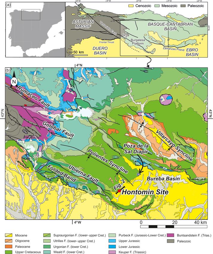
720                                              R. Pérez-López et al.: An active tectonic field for CO2 storage management

and earthquakes triggering, with the consequence of leakage            In this work, we propose that the description, the analy-
and seepage, and (2) the long-term reservoir behavior, under-       sis and establishment of the tectonic strain field have to be
standing long-term as a centennial to millennial time span.         mandatory for long-term GSC monitoring and management,
Therefore, what is the long-term behavior of GSC? What do           implementing the fault behavior in the geomechanical mod-
we need to monitor for safe GSC management? Winthaegen              els. This analysis does not increase the cost of long-term
et al. (2005) suggest three subjects for monitoring: (a) the        monitoring, given that it is low-cost and the results are ac-
atmosphere air quality near the injection facilities, due to        quired in a few months. Therefore, we propose a method-
the CO2 toxicity (values greater than 4 %; see Rice, 2003,          ology based on the reconstruction of the strain field from
and Permentier et al., 2017), (b) the overburden monitoring         the classical studies in geodynamics (Angelier, 1979, 1984;
faults and wells, and (c) the sealing of the reservoir. The         Reches, 1983, 1987). As an innovation, we introduce the
study of natural analogs for GSC is a good strategy to es-          strain field (SF) analysis between 20 km away from the sub-
timate the long-term behavior of the reservoir, considering         surface reservoir deep geometry, under the area of influence
parameters such as the injected CO2 pressure and volume,            of induced seismicity for fluid injection. The knowledge of
plus the brine mixing with CO2 (Pearce, 2006). Hence, the           the strain field at a local scale allows classifying the type of
prediction of site performance over long timescales also re-        faulting and their role for leakage processes, whilst the re-
quires an understanding of CO2 behavior within the reser-           gional scale explores the tectonically active faults that could
voir, the mechanisms of migration out of the reservoir, and         affect the reservoir. The methodology is rather simple, tak-
the potential impacts of a leak on the near-surface environ-        ing measures of slickensides and striations on fault planes to
ment. The assessments of such risks will rely on a combina-         establish the orientation of the maximum horizontal short-
tion of predictive models of CO2 behavior, including the fluid      ening (ey ) and the minimum horizontal shortening (ex ) for
migration and the long-term CO2 –porewater–mineralogical            the strain tensor. The principal advantage of the SF analy-
interactions (Pearce, 2006). Once again, the tectonically ac-       sis is the direct classification of all the faults involved in the
tive field interacts directly with this assessment. Moreover,       geomechanical model and the prediction of the failure pa-
the fault reactivation due to the pore pressure increasing dur-     rameters. Moreover, a Mohr–Coulomb failure analysis was
ing the injection and storage also has to be considered (Röh-       performed on the fault pattern recognized in the Cretaceous
mann et al., 2013). Despite the uplift measured by Röhmann          outcrop located on top of the pilot plant.
et al. (2013) being sub-millimeter (ca. 0.021 mm) at the end           The tectonic characterization of the GSC of Hontomín was
of the injection processes, given the ongoing occurrence of         implemented in the geological model described by Le Gallo
micro-earthquakes, long-term monitoring is required. The            and de Dios (2018). Beyond the use of induced seismicity
geomechanical and geological models predict the reservoir           and potentially active faults, the scope of this method is to
behavior and the caprock sealing properties. The role of the        propose an initial analysis to manage underground storage
faults inside these models is crucial for the tectonic long-        operations. We present how the structural analysis of fault or
term behavior and the reactivation of faults that could trigger     slip data can improve the knowledge on the tectonic large-
earthquakes.                                                        scale fault network for the potential seismic reactivation dur-
   Concerning induced seismicity, Wilson et al. (2017) pub-         ing fluid injection and the time-dependent scale of fluid stays.
lished the Hi-Quake database, with a classification of all
man-made earthquakes according to the literature, in an on-
line repository (https://inducedearthquakes.org/, last access:      2     Hontomín onshore case study
May 2019). This database includes 834 projects with proved
induced seismicity, where two different cases with earth-           2.1    Geological description of the reservoir
quakes as large as M = 1.7, detected in swarms of about
9500 micro-earthquakes, are related to GSC operations. Ad-          The CO2 storage site of Hontomín is enclosed in the southern
ditionally, Foulger et al. (2018) pointed out that GSC can          section of the Mesozoic Basque–Cantabrian Basin, known
trigger earthquakes with magnitudes less than M = 2: the            as the Burgalesa Platform (Serrano and Martínez del Olmo,
cases described in their work are as great as M = 1.8, with         1990; Tavani, 2012), within the sedimentary Bureba Basin
the epicenter location 2 km around the facilities. McNa-            (Fig. 1). This geological domain is located in the northern
mara (2016) described a comprehensive method and proto-             junction of the Cenozoic Duero and Ebro basins, forming an
col for monitoring a GSC reservoir for the assessment and           ESE-dipping monocline bounded by the Cantabrian Moun-
management of induced seismicity. The knowledge of active           tain Thrust to the north, the Ubierna Fault System (UFS) to
fault patterns and the stress or strain field could help design a   the south and the Asturian Massif to the west (Fig. 1).
monitoring network and identify those faults capable of trig-          The Meso-Cenozoic tectonic evolution of the Burgalesa
gering micro-earthquakes (M < 2) and/or breaking the seal-          Platform starts with a first rift period during Permian and
ing for leakage (patterns of open faults for low-permeability       Triassic times (Dallmeyer and Martínez-García, 1990; Cal-
CO2 migration).                                                     vet et al., 2004), followed by relative tectonic quiescence
                                                                    during Early and Middle Jurassic times (e.g., Aurell et al.,

Solid Earth, 11, 719–739, 2020                                                                 www.solid-earth.net/11/719/2020/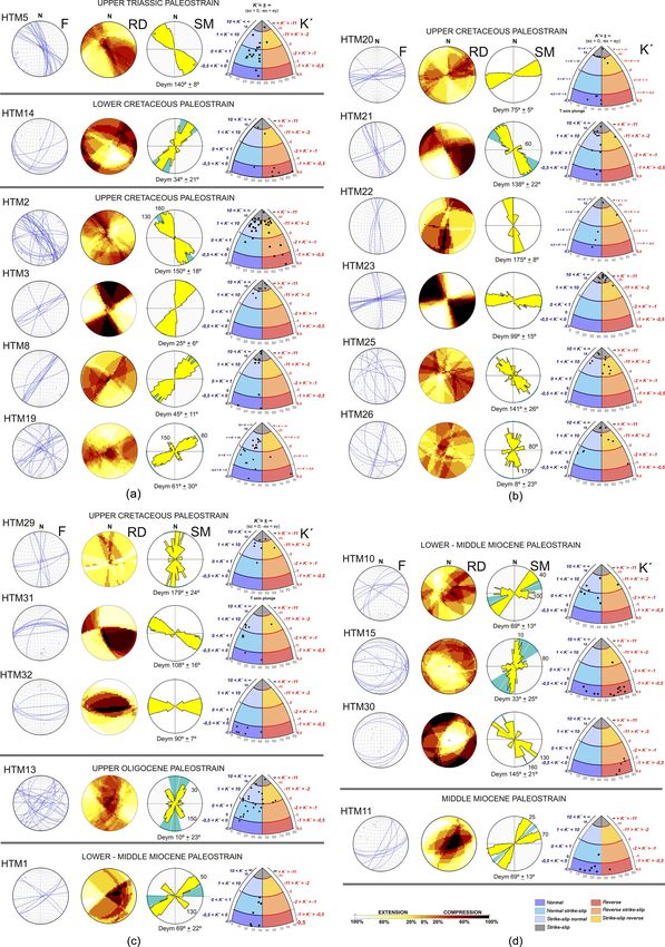
R. Pérez-López et al.: An active tectonic field for CO2 storage management                                                             721

Figure 1. (a) Location map of the study area in the Iberian Peninsula, along with the geological map of the Asturian and Basque–Cantabrian
areas, labeling major units and faults (modified after Quintà and Tavani, 2012); (b) geographical location of Hontomín pilot plant (red dot)
within the Basque–Cantabrian Basin. This basin is tectonically controlled by the Ubierna Fault System (UFS; NW–SE-oriented) and the
parallel Polientes syncline, the Duero and Ebro Tertiary basins, and Poza de la Sal evaporitic diapir. Cret: Cretaceous; F: facies.

2002). The main rifting phase took place during Late Juras-             ture is bordered by the UFS to the south and west, by the Poza
sic and Early Cretaceous times, due to the opening of the               de la Sal diapir and the Zamanzas Popup structure (Carola,
North Atlantic and the Bay of Biscay-Pyrenean rift system               2014) to the north, and by the Ebro Basin to the east (Fig. 1).
(García-Mondéjar et al., 1986; Le Pichon and Sibuet, 1971;              The structure is defined as a forced fold-related dome struc-
Lepvrier and Martínez-García, 1990; García-Mondéjar et al.,             ture (Tavani et al., 2013; Fig. 2), formed by an extensional
1996; Roca et al., 2011; Tugend et al., 2014). The conver-              fault system with migration of evaporites towards the hang-
gence between Iberia and Eurasia from Late Cretaceous to                ing wall during the Mesozoic (Soto et al., 2011). During
Miocene times triggered the inversion of previous Mesozoic              the tectonic compressional phase, associated with the Alpine
extensional faults and the development of an E–W orogenic               Orogeny affecting the Pyrenees, the right-lateral transpres-
belt (Cantabrian domain to the west and Pyrenean domain                 sive inversion of the basement faults was activated, along
to the east) formed along the northern Iberian plate margin             with the reactivation of transverse extensional faults (Fig. 2;
(Muñoz, 1992; Gómez et al., 2002; Vergés et al., 2002).                 Tavani et al., 2013; Alcalde et al., 2014).
   The Hontomín facilities are located within the Basque–                  The target reservoir and seal formations consist of Lower
Cantabrian Basin (Fig. 1b). The geological reservoir struc-             Jurassic marine carbonates, arranged in an asymmetric

www.solid-earth.net/11/719/2020/                                                                        Solid Earth, 11, 719–739, 2020
722                                               R. Pérez-López et al.: An active tectonic field for CO2 storage management

Figure 2. Interpretation of a 2-D seismic reflection profile crossing the oil exploration wells (H1, H2 and H4), along with the monitoring
well (Ha) and injection well (Hi) through Hontomín pilot plant (HPP). Modified from Alcalde et al. (2014). See Fig. 1 for location; black
line at the red circle.

dome-like structure (Fig. 2) with an overall extent of 15 km2                in the southeastward area, being active between the
and located at 1485 m depth (Alcalde et al., 2013, 2014;                     Permian and Triassic period and strike-slip during the
Ogaya et al., 2013). The target CO2 injection point is a saline              Cenozoic contraction. In this tectonic configuration, the
aquifer formed by a dolostone unit, known as “Carniolas”,                    Ubierna Fault acts as a right-lateral strike-slip fault.
and an oolitic limestone of the Sopeña Formation, both cor-                  These authors pointed out the sharp contacts between
responding to Lias in time (Early Jurassic). The estimated                   the thrusts and the strike-slip faults in this basin. Fur-
porosity of the Carniolas reaches over 12 % (Ogaya et al.,                   thermore, Tavani et al. (2011) also described a complex
2013; Le Gallo and de Dios, 2018), and it is slightly lower                  Cenozoic tectonic context where a right-lateral tectonic
at the Carbonate Lias level (8.5 % in average). The reser-                   style reactivated WNW-ESE-trending faults. Both the
voir levels contain saline water with more than 20 g L−1 of                  Ventaniella and the Ubierna faults acted as transpres-
NaCl and very low oil content. The high porosity of the lower                sive structures, 120 km long and 15 km wide and fea-
part of the reservoir (i.e., the Carniolas level) is the result of           turing 0.44 mm yr−1 averaged tectonic strike-slip defor-
secondary dolomitization and different fracturing events (Al-                mation between the Oligocene and the present day. The
calde et al., 2014). The minimum thickness of the reservoir                  aforementioned authors described different surface seg-
units is 100 m. The potential upper seal unit comprises Lias                 ments of the UFS of right-lateral strike-slip ranging be-
marlstones and black shales from a hemipelagic ramp (Fig. 2;                 tween 12 and 14 km length. The structural data collected
Pliensbachian and Toarcian) of the “Puerto del Pozazal” and                  by Tavani et al. (2011) pointed out that 60 % of data
Sopeña formations.                                                           correspond to right-lateral strike-slip with a WNW–
                                                                             ESE trend, together with conjugate reverse faulting with
2.2   Regional tectonic field                                                a NE–SW, NW–SE and E–W trend, and left-lateral
                                                                             strike-slip faults N–S-oriented. They concluded that this
The tectonic context has been described from two different                   scheme could be related to a transpressional right-lateral
approaches: (1) the tectonic style of the fractures bordering                tectonic system with a maximum horizontal compres-
the Hontomín reservoir (De Vicente et al., 2011; Tavani et                   sion, SHmax , striking 120◦ E. Concerning the geological
al., 2011) and (2) the tectonic regional field described from                evidence of recent sediments affected by tectonic move-
earthquakes with mechanism solutions and GPS data (Her-                      ments of the UFS, Tavani et al. (2011) suggest the mid-
raiz et al., 2000; Stich et al., 2006; De Vicente et al., 2008).             dle Miocene in time for this tectonic activity. However,
                                                                             geomorphic markets (river and valley geomorphology)
  1. The tectonic style of the Bureba Basin was described by                 could indicate tectonic activity at present times. All of
     De Vicente et al. (2011), which classified the Basque–                  these data correspond to regional or small-scale data
     Cantabrian Cenozoic Basin (Fig. 1a) as transpressional                  collected to explain the Basque–Cantabrian Cenozoic
     with a contractional horsetail splay basin. The NW–SE-                  transpressive basin. The advantage of the methodology
     oriented Ventaniella Fault (Fig. 1a) includes the UFS

Solid Earth, 11, 719–739, 2020                                                                     www.solid-earth.net/11/719/2020/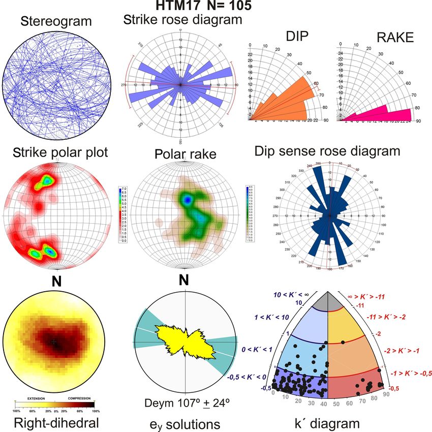
R. Pérez-López et al.: An active tectonic field for CO2 storage management                                                     723

      proposed here to establish the tectonic local regime af-     case of the Hontomín facilities. Moreover, this project claims
      fecting the reservoir is the search for local-scale tec-     to create a favorable environment for GSC onshore through
      tonics (with a size of 20 km) and the estimation of the      public engagement, knowledge sharing and training (Gastine
      depth for the non-deformation surface for strata folding     et al., 2017). In this context, the work-package WP1 is de-
      in transpressional tectonics (Lisle et al., 2009).           voted to “ensuring safe storage operations”.
 2. Regarding the stress field from earthquake focal mech-
    anism solutions, Herraiz et al. (2000) pointed out the         3     Methods and rationale
    regional trajectories of SHmax with a NNE–SSW trend,
    and with a NE–SW SHmax trend from slip-fault inver-            The lithosphere remains in a permanent state of deforma-
    sion data. Stich et al. (2006) obtained the stress field       tion, related to plate tectonic motion. Strain and stress fields
    from seismic moment tensor inversion and GPS data.             are the consequence of this deformation on the upper litho-
    These authors pointed out a NW–SE Africa–Eurasia               sphere, causing different fault patterns that determine sed-
    tectonic convergence at a tectonic rate of approximately       imentary basins and geological formations. The kinematics
    5 mm yr−1 . However, no focal mechanism solutions are          of these faults describe the stress or strain fields, for exam-
    found within the Hontomín area (20 km) and only long-          ple measuring grooves and slickensides on fault planes (see
    range spatial correlation could be made with high un-          Angelier, 1979, and Reches, 1983, among others). The rele-
    certainty (in time, space and magnitude). The same lack        vance of the tectonic field is that stress and strain determine
    of information appears in the work of De Vicente et            the earthquake occurrence by the fault activity. In this work,
    al. (2008), with no focal mechanism solutions in the           we have performed a brittle analysis of the fault kinematics
    50 km surrounding the Hontomín pilot plant (HPP). In           by measuring slickenfiber on fault planes (dip–dip direction
    this work, these authors classified the tectonic regime        and rake), in several outcrops in the surroundings of the on-
    as a uniaxial extension to strike-slip with a NW–SE            shore reservoir. To carry out the methodology proposed in
    SHmax trend.                                                   this work, the study area was divided into a circle with four
                                                                   equal areas, and we searched outcrops of fresh rock to per-
   Regional data about the tectonic field inferred from differ-    form the fault kinematic analysis. This allows establishing a
ent works (Herraiz et al., 2000; Stich et al., 2006; De Vicente    realistic tectonic very near field to be considered during the
et al., 2008, 2011; Tavani et al., 2011; Tavani, 2012) show        storage seismic monitoring and long-term management. Fi-
differences for the SHmax . These works explain the tectonic       nally, we have studied the fault plane reactivation by using
framework for the regional scale. Nevertheless, local tecton-      the Mohr–Coulomb failure criterion (Pan et al., 2016) from
ics could determine the low permeability and the potential         the fault pattern obtained in the Cretaceous limestone outcrop
induced seismicity within the reservoir. In the next section,      located on top of the HPP facilities.
we have applied the methodology described at Sect. 3 of this
paper, in order to compare the regional results from these         3.1    Paleostrain analysis
works.
                                                                   We have applied the strain inversion technique to reconstruct
2.3   Strategy of the ENOS European project                        the tectonic field (paleostrain evolution), affecting the Hon-
                                                                   tomín site between the Triassic, Jurassic, Cretaceous and
HPP for CO2 onshore storage is the only one in Europe rec-         Neogene ages (late Miocene to present times). For a further
ognized as a key test facility, and it is managed and conducted    methodological explanation, see Etchecopar et al. (1981),
by CIUDEN (Fundación Ciudad de la Energía). The HPP is             Reches (1983) and Angelier (1990). The main assumption
located within the province of Burgos (Fig. 1b), in the north-     for the inversion technique of fault population is the self-
ern central part of Spain.                                         similarity to the scale invariance for the stress or strain ten-
   The methodology proposed in this work and its applica-          sors. This means that we can calculate the whole stress or
tion for long-term onshore GSC management in the context           strain fields by using the slip data on fault planes and for ho-
of geological risk is based on the strain tensor calculation, as   mogeneous tectonic frameworks. The strain tensor is an el-
part of the objectives proposed in the European project EN-        lipsoid defined by the orientation of the three principal axes
abling Onshore CO2 Storage in Europe (ENOS). The ENOS              and the shape of the ellipsoid (k). This method assumes that
project is an initiative of CO2GeoNet, the European Network        the slip vectors, obtained from the pitch of the striation on
of Excellence on the geological storage of CO2 , to support        different fault planes, define a common strain tensor or a set
onshore storage and highlight the associated problems, such        in a homogeneous tectonic arrangement. We assume that the
as GSC perception, safe storage operation, potential leakage       strain field is homogeneous in space and time, the number
management, and health and environmental safety (Gastine           of faults activated is greater than five and the slip vector is
et al., 2017). ENOS combines a multidisciplinary European          parallel to the maximum shear stress (τ ).
project, which focuses in onshore storage, with the demon-
stration of best practices through pilot-scale projects in the

www.solid-earth.net/11/719/2020/                                                                 Solid Earth, 11, 719–739, 2020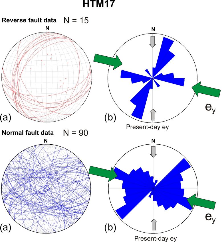
724                                              R. Pérez-López et al.: An active tectonic field for CO2 storage management

   The inversion technique is based on the Bott equations           orientation of the principal strain axes, ey , and, hence, the
(Bott, 1959). These equations show the relationship between         minimum stress axis, Shmin , is parallel to the minimum strain
the orientation and the shape of the stress ellipsoid:              axis, ex . This assumption allows us to estimate the stress tra-
                       h                  i                       jectories (SHmax and Shmin ) from the ey SM results.
tan(θ ) = [n/(l · m)] · m2 − 1 − n2 · R 0 ,             (1)            Resolving the equations of Anderson for different values
R 0 = (σz − σx ) / σy − σx ,

                                                        (2)         (Anderson, 1951), we can classify the tectonic regime that
                                                                    activates one fault from the measurement of the fault dip,
where l, m and n are the direction cosines of the normal to the     sense of dip (0–360◦ ) and pitch of the slickenside, assuming
fault plane, θ is the pitch of the striation and R 0 is the shape   that one of the principal axes (ex , ey or ez ) is vertical (Ange-
of the stress ellipsoid obtained in an orthonormal coordinate       lier, 1984). We can classify the tectonic regime and represent
system, x, y, z. In this system, σy is the maximum horizontal       the strain tensor by using the ey and ex orientation.
stress, σx is the minimum horizontal stress axis and σz is the
vertical stress axis.                                               3.4   The K 0 -strain diagram

3.2   The right-dihedral model for paleostrain analysis             Another analysis can be achieved by using the K 0 -strain di-
                                                                    agram developed by Kaverina et al. (1996) and codified in
The right-dihedral (RD) is a semiquantitative method based          Python code by Álvarez-Gómez (2014). These authors have
on the overlapping of compressional and extensional zones           developed a triangular representation based on the fault slip,
by using a stereographic plot. The final plot is an interfer-       where tectonic patterns can be differentiated as strike-slip
ogram figure, which usually defines the strain regime. This         and dip-slip types. This diagram is divided into seven dif-
method is strongly robust for conjugate fault sets and with         ferent zones according to the type of fault: (1) pure normal,
different dip values for the same tensor. The RD was orig-          (2) pure reverse and (3) pure strike-slip; these were com-
inally defined by Pegoraro (1972) and Angelier and Mech-            bined with the possibility of oblique faults ((4) reverse strike-
ler (1977), as a geometric method, adjusting the measured           slip and (5) strike-slip with a reverse component) and lateral
fault-slip data (slickensides) in agreement with theoretical        faults ((6) normal strike-slip and (7) strike-slip faults with a
models for extension and compressive fault slip. Therefore,         normal component; Fig. 3). Strike-slip faults are defined by
we can constrain the regions of maximum compression and             small values for pitch (p < 25◦ ) and dips close to vertical
extension related to the strain regime.                             planes (β > 75◦ ). High pitch values (p > 60◦ ) are related to
                                                                    normal or reverse fault-slip vectors. Extensional faults show
3.3   The slip model for the paleostrain analysis
                                                                    ey in the vertical, whereas compressional faults show ey in
The slip model (SM) is based on the Navier–Coulomb frac-            the horizontal plane.
turing criteria (Reches, 1983), taking the Anderson model so-          This method was originally performed for earthquake fo-
lution for this study (Anderson, 1951; Simpson, 1997). The          cal mechanism solutions by using the focal parameters, the
Anderson model represents the geometry of the fault plane as        nodal planes (dip and strike) and rake (Kaverina et al., 1996).
monoclinic, relating the quantitative parameters of the shape       The triangular graph is based on the equal-area representa-
parameter (K 0 ) with the internal frictional angle for rock me-    tion of the T , N , or B and P axes in spherical coordinates
chanics (ϕ) (De Vicente, 1988; Capote et al., 1991). More-          (T tensile, N or B neutral, and P pressure axes) and the or-
over, this model is valid for neoformed faults, and some con-       thogonal regression between earthquake magnitudes Ms and
siderations have to be accounted for for previous faults and        mb for the Harvard earthquake Global CMT (Centroid Mo-
weakness planes present in the rock. These considerations           ment Tensor) catalogue in 1996. Álvarez-Gómez (2014) pre-
are related to the dip of normal and compressional faults,          sented a Python-based for computing the Kaverina diagrams,
such as for compressional faulting dip values lower than 45◦ ,      and we have modified the input parameters by including the
reactivated as extensional faults. This model shows the rela-       K 0 intervals for the strain field from the SM. The relationship
tionships between the K 0 , ϕ and the direction cosines for the     between the original diagram of Kaverina (Fig. 3a) and the
striation on the fault plane (De Vicente, 1988; Capote et al.,      K 0 -strain diagram (Fig. 3b) that we have used in this work
1991):                                                              is shown in Fig. 3. The advantage of this diagram is the fast
                                                                    assignation of the type of fault and the tectonic regime that
K 0 = ey /ez ,                                               (3)    determines this fault pattern and the strain axes relationship.
where ez is the vertical strain axis, ey is the maximum hori-          Table 1 summarizes the different tectonic regimes of
zontal shortening and ex is the minimum horizontal shorten-         Fig. 3b showing the relationship with the strain main axes ey ,
ing. This model assumes that there is no change in volume           ex and ez . This diagram exhibits a great advantage to classify
during the deformation and ey = ex + ez .                           the type of fault according to the strain tensor. Therefore, we
   For isotropic solids, principal strain axes coincide with the    can assume the type of fault from the fault orientation affect-
principal stress axes. This means that in this work, the ori-       ing geological deposits for each strain tensor obtained.
entation of the principal stress axis, SHmax , is parallel to the

Solid Earth, 11, 719–739, 2020                                                                 www.solid-earth.net/11/719/2020/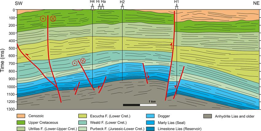
R. Pérez-López et al.: An active tectonic field for CO2 storage management 725
Figure 3. (a) Kaverina original diagram to represent the tectonic regime from an earthquake focal mechanism population (see Kaverina et
al., 1996, and Álvarez-Gómez, 2014). (b) K 0 -strain diagram used in this work. Dotted lines represent the original Kaverina limits. Colored
zones represent the type of fault. The tectonic regime is also indicated by the relationship between the strain axes and the colored legend.
SS: strike-slip. The B axis is orthogonal to the P and T axes.
Table 1. Different tectonic regimes, K 0 values, dip values and fault type for the Kaverina modified diagram used in this work. According to
the strain axes relationship, faults can be classified and the tectonic regime can be established.
K0 Dip Strain axis Fault type Tectonic field
< −0.5 0◦ ez > −ex = −ey normal pure radial extension
−0.5 < K 0 < 0 0–45◦ ez > −ex > ey normal radial extension
K0 = 0 0–45◦ ez = −ex ; ey = 0 normal plane deformation
0 < K0 < 1 0–45◦ −ex > ez > ey normal with SS extension with SS
K0 = 1 0–45◦ −ex > ey = ez normal with SS extension with SS
1 < K 0 < 10 0–45◦ −ex > ey > ez strike-slip with N SS with extension
10 < K 0 < ∞ 0–45◦ – strike-slip SS deformation
K0 = ∞ 45◦ ez = 0; −ex = ey strike-slip pure SS deformation
∞ < K 0 < −11 45–90◦ – strike-slip SS deformation
−11 < K 0 < −2 45–90◦ ey > −ex > −ez strike-slip with R SS with compression
K 0 = −2 45–90◦ ey > −ex = −ez reverse with SS compression with SS
−2 < K 0 < −1 45–90◦ ey > −ez > −ex reverse with SS compression with SS
K 0 = −1 45–90◦ −ez = ey ; ex = 0 reverse plane deformation
−1 < K 0 < −0.5 45–90◦ −ez > ey > ex reverse radial compression
K 0 = −0.5 45–90◦ −ez > ey = ex reverse pure radial compression
SS: strike-slip; ex = Shmin : minimum horizontal shortening; N: normal; ey = SHmax : maximum horizontal shortening; R: reverse
and ez : vertical axis.
3.5 The circular-quadrant-search (CQS) strategy for the orientation of the ey , ex and K 0 to plot on a map and,
the paleostrain analysis therefore, to establish the tectonic regime. We have chosen
quadrants of the circles with the aim to obtain a high-quality
spatial distribution of point for the interpretation of the local
In this work, we propose a low-cost strategy based on a well- and very near strain field. Hence, data are homogeneously
known methodology for determining the stress or strain ten- distributed, instead of being only concentrated in one quad-
sor affecting a GSC reservoir, which will allow the long-term rant of the circle.
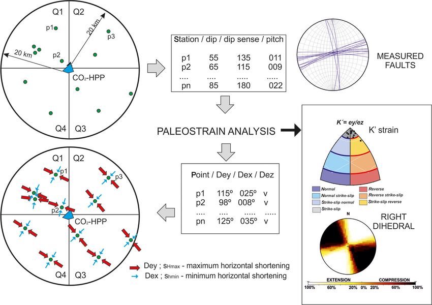
monitoring of geological and seismic behavior (Fig. 4). The Pérez-López et al. (2018) carried out a first approach to
objective is to obtain enough structural data and spatially ho- the application of this methodology at Hontomín, under the
mogeneous of faults (Figs. 4 and 5) for reconstructing the objective of the ENOS project (see next section for further
stress or strain tensor. The key point is the determination of
www.solid-earth.net/11/719/2020/ Solid Earth, 11, 719–739, 2020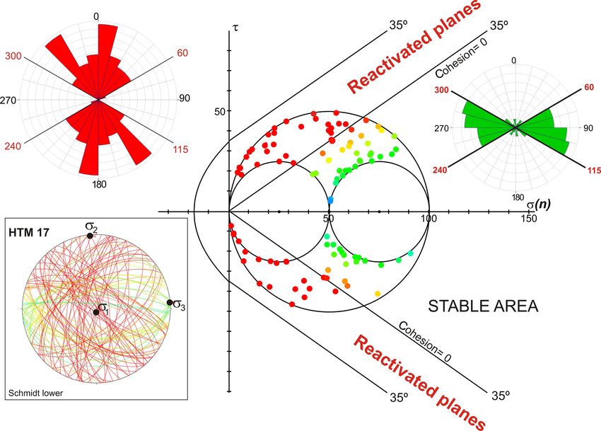
726                                               R. Pérez-López et al.: An active tectonic field for CO2 storage management

Figure 4. Methodology proposed to obtain the strain field affecting the GSC reservoir. The distances for outcrops and quadrants proposed is
20 km. The technique of right-dihedral and the K 0 -strain diagram is described in the main text. The ey and ex represented are a model for
explaining the methodology. Dey and Dex are the direction of the maximum and minimum strain, respectively. Blue box at the center is the
CO2 storage geological underground formation.

details). We propose a circular searching of structural field           2018), which is confined in folded and fractured deep geo-
stations (Figs. 4 and 5), located within a 20 km radius. This           logical structures, in which local tectonics plays a key role in
circle was chosen, given that active faults with the capac-             micro-seismicity and the possibility of CO2 leakage.
ity of triggering earthquakes of magnitudes close to M = 6                 The constraints of this strategy are related to the absence
exhibit a surface rupture of tens of kilometers, according to           of kinematic indicators on fault planes. This absence could
empirical models (Wells and Coppersmith, 1994). Moreover,               occur due to later overlapping geological processes as neo-
Verdon et al. (2015) pointed out that the maximum distance              formed mineralization. Also, a low rigidity eludes the slick-
of induced earthquakes for fluid injection is 20 km. Larger             enfiber formation, and no kinematic data will be marked on
distances could not be related to the stress or strain regime           the fault plane. A poor spatial distribution of the outcrops
within the reservoir, except for the case of large geological           was also taken into account for constraining the strategy. The
structures (folds, master faults, etc.). Microseismicity in GSC         age of sediments does not represent the age of the active de-
reservoir is mainly related to the operations during the injec-         formations, and, hence, the active deformation has to be ana-
tion or depletion stages and long-term storage (Verdon, 2014;           lyzed by performing alternative methods (i.e., paleoseismol-
Verdon et al., 2015; McNamara, 2016).                                   ogy, archaeoseismology).
   The presence of master faults (capable of triggering earth-
quakes of magnitude = or > than a 6 and 5 km long seg-
ment) inside the 20 km radius circle implies that the regional          4     Results
tectonic field determines the strain accumulation in a kilo-
metric fault size. Furthermore, the presence of master faults           4.1    Strain field analysis
could increase the occurrence of micro-earthquakes, due to
the presence of secondary faults prone to triggering earth-             We have collected 447 fault-slip data points on fault planes in
quakes by their normal seismic cycle (Scholz, 2018). It must            32 outcrops, located within a 20 km radius circle centered at
be borne in mind that GSC onshore reservoirs used to be deep            the HPP (Fig. 5). The age of the outcrops ranges from Early
saline aquifers (e.g., Bentham and Kirby, 2005) as in the case          Triassic to post-Miocene, and they are mainly located in Cre-
of Hontomín (Gastine et al., 2017; Le Gallo and de Dios,                taceous limestone and dolostone (Fig. 5, Table 2). However,

Solid Earth, 11, 719–739, 2020                                                                     www.solid-earth.net/11/719/2020/
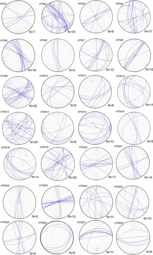
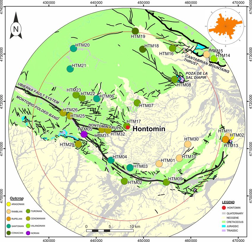
R. Pérez-López et al.: An active tectonic field for CO2 storage management                                                                727

Figure 5. Geographical location of field outcrops in the eastern part of the Burgalesa Platform domain. Black lines: observed faults; red
circle: 20 km radius study zone. Rose diagram are the fault orientations from the map. A total of 447 fault data were collected in 32 outcrops.
Data were measured by a tectonic compass on fault planes at outcrops. The spatial distribution of the field stations is constrained by the
lithology. Coordinates are in meters, UTM H30.

no Jurassic outcrops were located, and only seven stations                27, 28 with no quality data), and of these 29 stations, 21 were
are located on Neogene sediments, ranging between early                   analyzed with the paleostrain technique. Solutions obtained
Oligocene to middle–late Miocene. The small number of                     here are robust to establish the paleostrain field in each out-
Neogene stations is due to the mechanical properties of the               crop as the orientation of ey , SHmax (Fig. 7).
affected sediments, mainly poorly lithified marls and soft-                  The results obtained from the application of the paleostrain
detrital fluvial deposits. Despite that, all the Neogene sta-             method have been expressed in a stereogram, RD, SM and a
tions exhibit high-quality data with a number of fault-slip               K 0 -strain diagram (Fig. 7). The K 0 -strain diagram shows the
data ranging between 7 and 8, enough for a minimum quality                fault classification as normal faults, normal with strike-slip
analysis.                                                                 component, pure strike-slip, strike-slip with reverse compo-
   We have labeled the outcrops with the acronym HTM fol-                 nent and reverse faults (see Fig. 3). The main faults are lat-
lowed by a number (see Fig. 5 for the geographical location               eral strike-slips and normal faults, followed by reverse faults,
and Table 2 and Fig. 6 for the fault data). The station with the          strike-slips and oblique strike-slips faults. The results of the
highest number of faults measured is HTM17 with 105 faults                strain regime are as follows: (1) 43 % of extensional with
on Cretaceous limestone. Conjugate fault systems can be rec-              shear component; (2) 22 % of shear; (3) 13 % of compres-
ognized in most of the stations (HTM1, 3, 5, 7, 10, 14, 16,               sive strain (Lower Cretaceous and early–middle Miocene,
21, 23, 24, 25, 29, 30 and 32; Fig. 6), although there are a few          Table 2); (4) 13 % of pure shear and (5) 9 % of shear with
stations with only one well-defined fault set (6, 22, 32). We             compression strain field, although with the presence of five
have to bear in mind that the recording of conjugate fault sys-           reverse faults.
tems is more robust for the brittle analysis than recording iso-             In contrast, we can observe that there are solutions with
lated fault sets, better constraining the solution (Žalohar and           a double value for the ey , SHmax orientation: HTM1, 2, 10,
Vrabec, 2008). In total, 29 of 32 stations were used (HTM24,              11, 13, 15, 19, 26, and 30. The stations HTM3 and 23 (Up-

www.solid-earth.net/11/719/2020/                                                                          Solid Earth, 11, 719–739, 2020
728                                                 R. Pérez-López et al.: An active tectonic field for CO2 storage management

Figure 6. Stereographic representation (cyclographic plot in Schmidt net, lower hemisphere) of the fault planes measured in the field stations.
“n” is the number of available data for each geostructural station. HTM24, 27 and 28 are not included due to lack of data, and HTM17 is not
included due to the high number of faults.

Solid Earth, 11, 719–739, 2020                                                                        www.solid-earth.net/11/719/2020/
R. Pérez-López et al.: An active tectonic field for CO2 storage management                                                              729

Figure 7. Results of the paleostrain analysis obtained and classified by age. Deym: striking of the averaged of the Dey value; F: fault
stereographic representation; K 0 -strain diagram with dots for each fault-slip solution; RD: right-dihedral method; SM: slip method. See the
Methods section for further explanation.
www.solid-earth.net/11/719/2020/                                                                        Solid Earth, 11, 719–739, 2020
730 R. Pérez-López et al.: An active tectonic field for CO2 storage management
Table 2. Summary of the outcrops showing the number of faults, the type of the strain tensor obtained, the Dey , SHmax striking and the age
of the affected geological materials. N-C is the normal component for strike-slip movement.
Station No. faults Series or epoch Dey (◦ ) Dispersion Strain tensor
HTM11 8 Middle Miocene 50 4 Normal strike-slip
HTM30 6 Early–middle Miocene 145 21 Compression
HTM15 13 Early–middle Miocene 33 25 Compression
HTM10 8 Early–middle Miocene 69 13 Normal strike-slip
HTM01 7 Early–middle Miocene 70 22 Normal strike-slip
HTM13 24 Early Oligocene 25–160 23 Normal strike-slip
HTM32 6 Upper Cretaceous 90 7 Normal
HTM31 11 Upper Cretaceous 108 16 Normal strike-slip
HTM29 8 Upper Cretaceous 179 24 Normal strike-slip
HTM26 10 Upper Cretaceous 0 23 Strike-slip
HTM25 11 Upper Cretaceous 141 26 Compression strike-slip
HTM23 14 Upper Cretaceous 99 15 Strike-slip
HTM22 5 Upper Cretaceous 175 8 Normal strike-slip
HTM21 14 Upper Cretaceous 138 22 Normal strike-slip
HTM20 11 Upper Cretaceous 75 5 Strike-slip
HTM19 20 Upper Cretaceous 61 30 Normal strike-slip
HTM17 105 Upper Cretaceous 107 24 Normal
HTM08 10 Upper Cretaceous 45 11 Strike-slip
HTM3 8 Upper Cretaceous 25 6 Strike-slip (N-C)
HTM2 34 Upper Cretaceous 150 18 Strike-slip (N-C)
HTM14 8 Lower Cretaceous 34 21 Compression
HTM5 18 Upper Triassic 140 8 Normal strike-slip
per Cretaceous) show the best solution for a strike-slip strain Cretaceous age, showing a compressive tectonic stage with
field as a pure strike-slip regime and ey with a 25 and 99◦ E reverse fault solutions, defined by ey with a NE–SW trend
trend, respectively (Fig. 7). (Fig. 7a–c). Taking into account the extensional stage related
It is easy to observe the agreement between the ey results to the main rifting stage that took place in Early Cretaceous
from the SM and the K 0 -strain diagram; for instance, in the times (i.e., Carola, 2014; Tavani, 2012; Tugend et al., 2014),
HTM2 the K 0 -strain diagram indicates strike-slip faults with we interpreted these results as a modern strain field, probably
a reverse component for low dips (0◦ < β < 40◦ ) but also in- related to the Cenozoic inversion stage.
dicates strike-slip faults with a normal component for larger Outcrops HTM2, 3, 8, 17, 19, 20, 21, 22, 23, 25, 26, 29,
dips (40◦ < β < 90◦ ). However, both results are in agree- 31 and 32 are from the Upper Cretaceous carbonates (Fig. 7).
ment with a strain field defined by the orientation for ey , Results are as follows: (1) a compressive strain stage featured
SHmax with 150◦ ± 18◦ trend. This tectonic field affects Cre- by ey with a NW–SE trend, similar to the stage described in
taceous carbonates and coincides with the regional tectonic Tavani (2012), and (2) a normal strain stage with ey strik-
field proposed by Herraiz et al. (2000), Tavani et al. (2011) ing both E–W and NE–SW (Fig. 7, HTM20, 21, 31 and 32).
and Alcalde et al. (2014). Finally, a (3) shear stage (activated strike-slip faults) and
(4) a shear with extension (strike-slip with normal compo-
4.2 Late Triassic outcrop paleostrain nent) were described as well. These two late stages are fea-
tured by ey with NE–SW and NW–SE trends. The existence
Strain analysis from the HTM5 fault set shows ey with a of four different strain fields is determined by different ages
NW–SE-trending and shear regime with the extension de- during the Cretaceous and different spatial locations in rela-
fined by strike-slip faults (Fig. 7a). This is in agreement with tion to the main structures, the Ubierna Fault System, Hon-
the uniaxial extension described in Tavani (2012), constrain- tomín Fault, Cantabrian Thrust, Montorio folded band and
ing this regime with SHmin with a NE–SW trend. the Polientes syncline (Fig. 1).
4.3 Cretaceous outcrop paleostrain
4.4 Cretaceous outcrop HTM17 on the Hontomín pilot
We have divided this result in two groups: (a) outcrops within plant
the 20 km circle from HPP and (b) the outcrop of the HTM17
(Fig. 5), which is located in the HPP facilities and described This outcrop is located on top of the geological reservoir, in
in the next section. HTM14 is the only outcrop of Early a quarry of Upper Cretaceous limestones. The main advan-
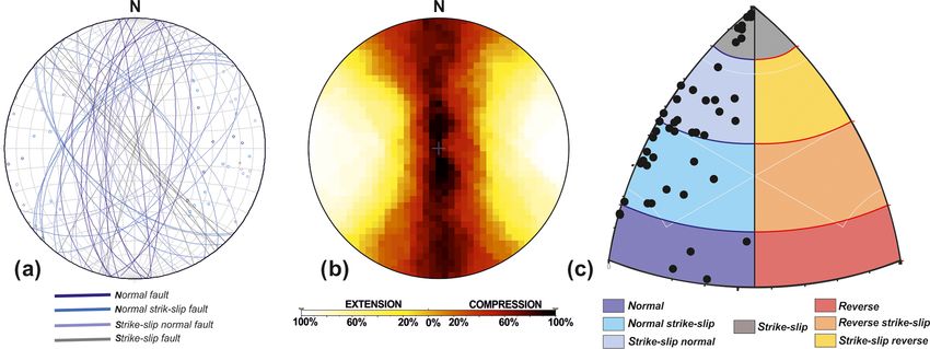
Solid Earth, 11, 719–739, 2020 www.solid-earth.net/11/719/2020/R. Pérez-López et al.: An active tectonic field for CO2 storage management 731
Figure 8. Fault data from the outcrop HTM17 located on top of the HPP. See Fig. 5 for the geographical location. Stereogram plot is lower
hemisphere and Schmidt net.
tage of this outcrop is the good development of striation and could be a reflex of the fracture network affecting the Jurassic
carbonate microfibers which yields high-quality data. Over- storage rocks at depth (see Figs. 2 and 9).
all, 105 fault-slip data were measured, with the main orien-
tation striking 75,−50 ◦ E and a conjugate set with a 130◦ E 4.5 Cenozoic outcrop strain field
(±10◦ ) trend (Fig. 8). The result of the strain inversion tech-
nique shows an extensional field featuring an ey trajectory The Cenozoic tectonic inversion in the area has been widely
striking 107◦ E (±24◦ ) related to an extensional strain field described by different authors (e.g., Carola, 2014; Tavani,
(see the K 0 -strain diagram in Fig. 8). Most of the faults are 2012; Tungend et al., 2014). This tectonic inversion is related
extensional faults NE–SW and NW–SE-oriented (Fig. 9), in to compressive structures, activating NE–SW and ENE–
agreement with the extensional RD solution. Reverse faults WSW thrusts with NW–SE and NNE–SSW ey trends, re-
are oriented NNE–SSW, E–W and WNW–ESE. The advan- spectively. The Ubierna Fault has been inverted with right-
tage of this outcrop is the geographical and stratigraphic po- lateral transpressive kinematics during the Cenozoic (Tavani
sition. It is located on top of the HPP facilities in younger et al., 2011). The Early Oligocene outcrop (HTM13, Fig. 7c)
sediments than the reservoir rocks. Furthermore, given that shows a local extensional field with ey with a NNE–SSW and
the Jurassic reservoir rock and the Cretaceous upper unit are 150◦ E trend. During the lower–middle Miocene, HTM15
both composed of carbonates, the fault pattern measured here and HTM30 outcrops exhibit the same ey trend, but for a
compressive tectonic regime (Fig. 7d). HTM1 shows exten-
www.solid-earth.net/11/719/2020/ Solid Earth, 11, 719–739, 2020732 R. Pérez-López et al.: An active tectonic field for CO2 storage management
al. (2014) shows ey , SHmax with almost NNW–SSE and N–S
trends. Namely, the work from Herraiz et al. (2000) calcu-
lates three stress tensors within the 20 km of our study area
and a Quaternary stress tensor close to the area (ca. 40 km
south of Hontomín). The age of the first one is Miocene and
defined by σ1 87/331◦ ; σ2 01/151◦ ; σ3 00/061◦ (dip–dip
sense 0–360◦ ), with an R = 0.06 and SHmax trending 151◦ E,
under an extensional tectonic regime. Two post-Miocene
stress tensors are defined by (1) σ1 87/299◦ ; σ2 00/209◦ ;
σ3 01/119◦ with R = 0.13, SHmax with a 29◦ E trend under an
extensional tectonic regime and (2) σ1 00/061◦ ; σ2 86/152◦ ;
σ3 03/331◦ , with R = 0.76, and SHmax 62◦ E under a strike-
slip tectonic regime. Finally, these authors calculated a Qua-
ternary stress tensor defined by σ1 85/183◦ ; σ2 02/273◦ ;
σ3 03/003◦ ; R = 0.02 and SHmax with a 101◦ E trend un-
der an extensional tectonic regime. The regional active stress
tensor defined for Pliocene–Quaternary ages is σ1 88/197◦ ;
σ2 01/355◦ ; σ3 00/085◦ for 327 data with R = 0.5 and
SHmax with an N–S trend under an extensional tectonic re-
gional regime.
We have applied the regional active stress tensor (Herraiz
et al., 2000) for studying the reactivation of previous fault
patterns measured in HTM17 (Figs. 8 and 9). To carry out
Figure 9. Normal and reverse faults stereograms (lower hemisphere
and Schmidt net), and rose diagrams measured in HTM17. Green
this study, we assume that the fault plane reactivation de-
arrows indicate the orientation of the local paleostrain field. Grey ar- pends on σ1 and σ3 and the shape of the failure envelope.
rows indicate the orientation of the present-day regional stress field Therefore, we have used the Mohr–Coulomb failure criteria
(Herraiz et al., 2000). for preexisting fault planes (Xu et al., 2010; Labuz and Zang,
2012), by using the MohrPlotter v3.0 code (Allmendinger et
al., 2012). Moreover, to calculate the Mohr–Coulomb circle,
sional tectonics with ey oriented 50 and 130◦ E. Summariz- it is necessary to know the cohesion and friction parameters
ing, the Cenozoic inversion and tectonic compression are de- of the reservoir rock. Bearing in mind that the reservoir rocks
tected during the early to middle Miocene and the Oligocene. are Lower Jurassic carbonates (dolostone and oolitic lime-
However, during the middle Miocene only one extensional stone; Alcalde et al., 2013, 2014; Ogaya et al., 2013), we
stage was interpreted (HTM1, Fig. 7c). have assumed the averaged cohesion for carbonates (lime-
The outcrops located closer to the HPP (HTM17, 31, 32, stone and dolostone) at 35◦ and the coefficient of internal
Figs. 5 and 7) show E–W faults. HTM5 is located on the friction of 0.7 (Goodman, 1989). In addition, we have as-
Ubierna Fault, showing a NW–SE trend, whilst HTM3 shows sumed no cohesion with an angle of static friction of 0.7 for
NE–SW strike-slip. preexisting faults.
Strain analysis suggests that the planes parallel to the Figure 10 shows the main results for the Mohr analysis.
SHmax orientation (NNW–SSE and N–S) could induce the The reactivated planes under the active present stress field
leakage into the reservoir (Fig. 7). Moreover, a 50◦ E are red dots: 52 of the original 105 fault-slip measurements
SHmax orientation could also affect the reservoir. HPP facili- at HTM17. Green and orange dots indicate faults with no
ties are close to the Hontomín Fault (Fig. 5), a WNW–ESE- tectonic strength accumulation under the present-day stress
oriented fault, although the HTM17 station shows that N–S field. Reactivated fault sets are oriented between N to 60◦ E
fault planes could play an important role for seepage of fluid and 115 to 180◦ E, with N–S and NNE–SSW as the main
into the reservoir. trends (Fig. 10, red rose diagram). Under an extensional tec-
tonic field with R = 0.5, N–S are normal faults, whereas
NNE–SSW and NNW–SSE trends are strike-slips faults with
5 Discussion extensional components. According to the results shown in
Fig. 10, these faults could be reactivated without a pore pres-
5.1 Regional active stress tensor in HTM17 fault sure increase. The inactive fault orientation is constrained be-
pattern tween 60 and 115◦ E, mainly WNW–ESE (Fig. 10, green rose
diagram). Regarding the uncertainties of these fault orienta-
The active regional field proposed by Herraiz et al. (2000), tions, these values can oscillate ±5◦ , according to the field
Stich et al. (2006), Tavani et al. (2011) and Alcalde et
Solid Earth, 11, 719–739, 2020 www.solid-earth.net/11/719/2020/R. Pérez-López et al.: An active tectonic field for CO2 storage management 733 Figure 10. Mohr–Coulomb failure analysis for the fault-slip data measured in HTM17 under the present-day stress tensor determined by Herraiz et al. (2000). Red dots are faults reactivated, and green and orange dots are located within the stable zone. Red rose diagram shows the orientation of reactivated faults, between N–S and 60◦ E and from 115 to 180◦ E. Green rose diagram shows the fault orientation for faults non-reactivated under the active stress field within the area. See text for further details. The yellow data in the Mohr–Coulomb (M–C) diagrams refer to those planes close to being reactivated and potentially reactivated by increasing the pore pressure. error measurement (averaged error for measuring structures σ2 = 01/355◦ and σ1 vertical. However, strain analysis in by a compass). this case shows a strike-slip extensional tectonic regime in- Concerning the reliability of the results, some constraints stead of the extensional regime derived from the stress field. need to be explained. The Mohr–Coulomb failure criterion Despite this, both the Mohr–Coulomb analysis and the pale- is an approximation that assumes that the normal stress on ostrain analysis (SM and RD) suggest N–S normal faulting, the fault plane is not tensile. Furthermore, the increases in NNE–SSW to NE–SW and NNW–SSE to NW–SE strike- pore pressure in the reservoir rock reduces the normal stress slips as the active fault network affecting the reservoir. De Vi- on the plane of failure, and the interval of fault reactivation cente et al. (1992) pointed out that the SM analysis is more could be higher. This effect was not considered in the pre- robust applied to fault-slip data classified previously by other vious analysis since the calculation of the critical pore pres- techniques. Here, we have used the Mohr–Coulomb failure sure is beyond the purpose of this work. Nevertheless, the criteria to separate active fault sets under the same strain ten- MohrPlotter software (Allmendinger et al., 2012) allows es- sor, yielding robustness to the results from SM and RD anal- timating the increase of pore pressure to the critical value ysis. under some conditions. We propose as complementary and future work a com- Finally, we have applied the slip model and right-dihedral bined analysis consisting of the fault population analysis and to the reactivated fault-slip data from the HTM17 outcrop the slip-tendency analysis (Morris et al., 1996), which could (Fig. 11), by including the rake estimated from the active improve and identify those fault sets most likely to be reac- regional stress tensor determined by Herraiz et al. (2000). tivated under an active stress field. Although both analyses At a glance, faults oriented between 10◦ E and 10◦ W act as (fault population and slip tendency) are based on the stress normal faults (4 out 52, Fig. 11a and c), faults between 10– tensor and the orientation of fault traces, the slip tendency 50◦ E and 10–50◦ W act as extensional faults with strike-slip also includes rock strength values obtained from the “in situ” components (31 out 52), and NE–SW and NW–SE vertical tests. faults act as pure strike-slips (8 out 52). The right-dihedral shows a tectonic regime of strike-slip with extensional com- 5.2 Active faulting in the surroundings of HPP ponent (see De Vicente et al., 1992), with orthorhombic symmetry and SHmax oriented 10◦ W, which is in agreement Quaternary tectonic markers for the UFS are suggested by with the stress tensor proposed by Herraiz et al. (2000) with Tavani et al. (2011). According to the tectonic behavior of www.solid-earth.net/11/719/2020/ Solid Earth, 11, 719–739, 2020
734                                                R. Pérez-López et al.: An active tectonic field for CO2 storage management

Figure 11. (a) Stereogram and poles of fault sets (HTM17) reactivated under the present-day stress field suggested by Herraiz et al. (2000).
(b) right-dihedral of the reactivated fault sets. (c) K 0 -strain diagram showing the type of fault for each fault set.

this fault as a right-lateral strike-slip and the fault segments        ment for the Ubierna Fault System, assuming surface rupture
proposed by Tavani et al. (2011), ranging between 12 and                segments between 12 and 14 km (Tavani et al., 2011). The
14 km long, the question is whether this fault could trigger            obtained results show that the maximum expected earthquake
significant earthquakes and what the maximum associated                 ranges between M = 6.0 and M = 6.1. For these fault pa-
magnitude could be. This is a relevant question given that the          rameters, Wells and Coppersmith (1994) indicate a total area
“natural seismicity” in the vicinity could affect the integrity         rupture ranging between 140 and 150 km2 . A surface fault
of the caprock. Bearing in mind the expected long life for the          trace rupture as lower as 7 km needs at least 20 km depth in
reservoir, estimated in thousands of years, the potential nat-          order to reach a value of the fault area rupturing greater than
ural earthquake that this master fault could trigger has to be          100 km2 , in line with a Moho between 36 and 40 at depth.
estimated. In this sense, it is necessary to depict seismic sce-           Regarding the instrumental earthquakes recorded into the
narios related to large earthquake triggering; however, this            area, the two largest earthquakes recorded correspond to
type of analysis is beyond the focus of this work.                      magnitude M = 3.4 and M = 3.3, with a depth ranging be-
   The incoming information that we have to manage in the               tween 8 and 11 km, respectively, and a felt macroseismic
area of influence (20 km) is (a) the instrumental seismicity,           intensity of III (EMS98, http://www.ign.es/web/ign/portal,
(b) the geometry of the fault, (c) the total surface rupture,           last access: May 2019). Both earthquakes occurred between
(d) the upper crust thickness and (e) the heat flow across the          50 and 60 km of distance from the Hontomín pilot plant.
lithosphere. Starting with the heat-flow value, the Hontomín            Only five earthquakes have been recorded within the 20 km
wells show a value that lies between 62 and 78 mW m−2 at                radius area of influence and with small magnitudes ranging
1500 m depth approximately (Fernández et al., 1998). Re-                between M = 1.5 and M = 2.3. The interesting data are the
garding the Moho depth in the area, these aforementioned au-            depth of these earthquakes, ranging between 10 and 20 km,
thors obtained a value ranging between 36 and 40 km depth,              which suggest that the seismogenic crust could reach 20 km
while the lithosphere base ranges between 120 and 130 km                depth.
depth (Torne et al., 2015). The relevance of this value is
the study of the thermal weakness in the lithosphere that               5.3    Local tectonic field and induced seismicity
could nucleate earthquakes in intraplate areas (Holford et al.,
2011). For these authors, the comparison between the crustal            The fluid injection into a deep saline aquifer, which is used
heat flow in particular zones, in contrast with the background          as GSC, generally increases the pore pressure. The increas-
regional value, could explain high seismicity and high rates            ing of the pore pressure migrates from the point of injection
of small-earthquake occurrence, as is the case of the New               to the whole reservoir. Moreover, changes in the stress field
Madrid Seismic Zone (Landgraf et al., 2018). For example,               for faults that are located below the reservoir could also trig-
in Australia heat-flow values of as much as 90 mW m−2 are               ger induced earthquakes (Verdon et al., 2014). Nevertheless,
related to earthquakes sized M > 5 (Holford et al., 2011).              to understand this possibility and the study, the volumetric
   Regarding the maximum expected earthquake into the                   strain field spatial distribution is required (Lisle et al., 2009).
zone, we have applied the empirical relationships obtained                 We have applied a physical model to estimate the total
by Wells and Coppersmith (1994). We have used the equa-                 volume injected (room conditions) in reservoir conditions.
tions for strike-slip earthquakes according to the strain field         Then we have applied McGarr’s (2014) approximation of
obtained in the area (pure shear), and the surface rupture seg-         the maximum expected seismic moment for induced earth-
                                                                        quakes. The injection of 10 kt of CO2 in Hontomín (Gastine

Solid Earth, 11, 719–739, 2020                                                                      www.solid-earth.net/11/719/2020/
You can also read