The Exomoon Corridor for Multiple Moon Systems
←
→
Page content transcription
If your browser does not render page correctly, please read the page content below
MNRAS 000, 1–19 (2020) Preprint 28 June 2021 Compiled using MNRAS LATEX style file v3.0

 The Exomoon Corridor for Multiple Moon Systems

 Alex
 1
 Teachey1★
 Academia Sinica Institute of Astronomy and Astrophysics
 11F of AS/NTU Astronomy-Mathematics Building, No.1, Sec. 4, Roosevelt Rd, Taipei 10617, Taiwan, R.O.C.

 Accepted 2021 June 24. Received 2021 June 8; in original form 2021 April 7
arXiv:2106.13421v1 [astro-ph.EP] 25 Jun 2021

 ABSTRACT
 Recently Kipping 2021 identified the so-called “exomoon corridor”, a potentially powerful
 new tool for identifying possible exomoon hosts, enabled by the observation that fully half of
 all planets hosting an exomoon will exhibit transit timing variation (TTV) periodicities of 2-4
 epochs. One key outstanding problem in the search for exomoons, however, is the question of
 how well the methods we have developed under the single moon assumption extend to systems
 with multiple moons. In this work we use -body simulations to examine the exomoon
 corridor effect in the more general case of ≥ 1 moons, generating realistic TTVs produced
 by satellite systems more akin to those seen in the outer Solar System. We find that indeed the
 relationship does hold for systems with up to 5 moons in both resonant and non-resonant chain
 configurations. Our results suggest an observational bias against finding systems with large
 numbers of massive moons; as the number of moons increases, total satellite mass ratios are
 generally required to be significantly lower in order to maintain stability, or architectures must
 be more finely tuned to survive. Moons produced in impact or capture scenarios may therefore
 dominate early detections. Finally, we examine the distribution of TTV periods measured for
 a large number of Kepler objects of interest (KOIs) and find the same characteristic exomoon
 corridor distribution in several cases. This could be dynamical evidence for an abundance of
 moons in the field, though we caution against strong inferences based on this result.
 Key words: planets and satellites: detection

 1 INTRODUCTION due to their small amplitudes, and TTVs by themselves have many
 other possible causes. This is unfortunate, because TTVs can often
 As the search for exomoons continues, so too does the search for
 be measured to high precision, so we would certainly like to be able
 powerful new tools to identify them. For a variety of reasons, time-
 to utilize this information, not only in the course of vetting moon
 domain photometry remains our best bet for detecting exomoons at
 system candidates, but also in identifying those candidates in the
 present: with missions like Kepler (Borucki et al. 2010) and TESS
 first place.
 (Ricker et al. 2015), there is an abundance of data available for a
 broad moon search. Moreover, time-domain photometry can in ideal To that end, Kipping 2021 (hereafter K21) recently identified
 circumstances reveal three distinct but self-consistent signatures a phenomenon called the “exomoon corridor”, in which exomoons,
 of exomoons: moon transits, transit timing variations (TTVs), and regardless of their underlying semimajor axis distribution, manifest
 transit duration variations (TDVs) (e.g. Sartoretti & Schneider 1999; predominantly short TTV periodicities. Because moon orbits will
 Szabó et al. 2006; Cabrera & Schneider 2007; Kipping 2009a,b). be undersampled – the period of the moon S will always be shorter
 In general, none of these signals on their own would be quite than the period of the planet P (Kipping 2009a) – the periods we
 enough to claim an unambiguous moon detection; we would ordinar- measure will always be aliases of the underlying oscillation signal.
 ily want to see at least two of these signals providing corroborative This is potentially a very useful observation, not only because
 evidence for a moon. For example, several putative moon transits TTVs are relatively easy to measure, but also because this distribu-
 with physically plausible associated TTVs could be convincing. Or, tion, with 50% of all exomoon systems showing periodicities of 2-4
 the combination of TTVs and TDVs, with the same period, expected epochs, appears distinct from the distribution of TTV induced by
 phase shift (Kipping 2009a,b; Heller et al. 2016), and amplitudes planet-planet interactions. For comparison, K21 computed TTVs
 suggesting a common mass and semimajor axis solution, might be for 90 known planet pairs (180 planets) investigated by Hadden &
 compelling, even if the moon’s transit is in the noise or missing Lithwick 2017 (henceforth HL2017), and found that by contrast only
 entirely. Unfortunately, TDVs are exceptionally difficult to measure 1% of these systems display such short-period TTV solutions. Thus,
 if we happen to measure a TTV with a period between two and four
 cycles, this system is immediately of interest because planet-planet
 ★ E-mail: amteachey@asiaa.sinica.edu.tw perturbation – probably the least exotic explanation available – is

 © 2020 The Authors

2 A. Teachey
comparatively far less likely (though not 50 times less likely; see constructing the simulated observations, and performing quality
K21 for further discussion on this interpretation). controls. In section 4 we report our results, including a diagnosis
 A lingering challenge, however, is the problem of systems with of the stability of these systems and their detectability. Section 5
multiple moons. The single moon assumption has been built in to discusses the impact of the results and examines the distribution
the K21 analysis, and indeed has been central to most exomoon pho- of TTVs for our simulated moon systems against the transit tim-
tometric search efforts to date (e.g. Kipping et al. 2012; Teachey & ings measured with Kepler photometry by Holczer et al. 2016. We
Kipping 2018; Alshehhi et al. 2020; Fox & Wiegert 2021). This is in conclude in section 6.
part because the inclusion of each subsequent moon requires seven
additional model parameters, and so as we add additional moons
it very quickly becomes computationally demanding to compute 2 THEORY
Bayesian evidences. Moreover, we quickly enter a regime in which
the data are simply insufficient to support such a complex model. The exomoon corridor result is based on the aliasing of moon signals
 This is problematic, because while the system is formally, as manifested in the Lomb-Scargle periodogram (Lomb 1976; Scar-
mathematically more complex, it is not really more complex in gle 1982). For the exomoon case, the phenomenon arises because
the sense of requiring significant additional credulity. That is, the the barycentric oscillation of the planet induced by the moon’s grav-
presence of multiple moons in a system does not so strain the itational tug is always higher frequency than the sampling cadence
imagination that we require overwhelming evidence for it; it may (Kipping 2009a) which, because we are measuring transit timings,
be equally or even more probable a priori. But in the prevailing is dictated by the orbital frequency of the planet. The result is an
framework we will penalize each additional moon for the extra undersampled signal with an aliased period given in K21 by
complexity – the data simply cannot support it, unless we can factor
in the relative probabilities of these different architectures, which 1
 TTV = . (1)
are at present poorly constrained. Thus, we may be biasing ourselves
 h i
 1 − round 1
against the detection of multi-moon systems.

 Furthermore, while the single moon case can be reasonably ap- With this straightforward expression we can produce Figure 1, which
proximated as a nested-two body problem, the presence of multiple maps the aliased signal TTV as a function of the period of the
moons means there will be more complicated dynamical interac- planet and the satellite . Below the TTV map we histogram
tions at play – not just multiple gravitational forces acting on the the distribution of these aliased periods and find the characteristic
planet, but also mutual interactions of the moons with one another pile-up at short periods found in K21. This simple picture then
– which can only be simulated properly through −body integra- suggests that there is an exact solution to this problem, and that we
tions. A simple model, comprised of a superposition of multiple might even be able to back out the true period of the moon from a
sinusoids, could of course be computed analytically for any config- given measurement of TTV and . Unfortunately, as K21 points
uration of moons, but the stability of these systems is not a given. out, and as the map shows, there are effectively infinite solutions
We must produce a realistic sample of these systems if we hope to for a given value of that will produce the observed TTV .
make inferences about the population. It would be possible to break this degeneracy, at least to a
 One notable exception to the single moon paradigm in the lit- point; there are not really infinite choices for . We could do better
erature was Heller et al. 2016, who examined the effect multiple by modeling the stability of the system in question to determine
moons would have on both TTVs and TDVs, and found that these plausible solutions, establishing a possible mass range for the
systems certainly do look significantly different than single-moons planet and/or moon based on transit depths (or upper limits on size
systems in TTV-TDV diagrams. While in the single-moon case, a based on non-detections), and / or incorporating the measurement
moon will trace out an ellipse in TTV-TDV space, multiple moons of (or upper limits on) TDVs. This is demanding work, but there is
will trace a more complex morphology. Unfortunately, the authors no getting around these additional efforts to better constrain , it
concluded these patterns would not be detectable with current in- simply does not fall out of the equation above.
struments, largely due to the aforementioned low signal-to-noise Further complicating the matter is the fact that the analytical
ratio (SNR) for TDVs with current facilities. TTV formula above cannot account for the presence of multiple
 In the short term, then, if we wish to use dynamical signatures aliases or harmonics within the periodogram. These do not show
to search for possible exomoon hosts, we will have to rely on lever- up in the K21 analysis, as that work does not grapple with the con-
aging TTVs by themselves. Hence the great promise of the exomoon founding issues of missing transits (making the sampling irregular),
corridor. and the presence of timing uncertainties. For real observations these
 In this work we investigate whether the exomoon corridor find- will certainly be a factor.
ing holds for the more general case of ≥ 1 moon systems. Consid- The system clearly has one ground truth solution for both
ering the additional dynamical complexity of multiple moons, it is and , but Lomb-Scargle periodograms typically manifest
by no means obvious that the single-moon assumption holds in the several peaks associated with a single signal, arising from the finite
very plausible context of a planet hosting more than one moon. Of sampling of the signal. For a well- and uniformly-sampled signal
course, the majority of massive moons in our Solar System (those with little or no noise, these peaks are typically, but not always,
that are potentially detectable by an extrasolar Kepler or Hubble strongest at the fundamental frequency. On the other hand, the peak
analog) are found in multi-moon systems, so it is quite reasonable power may not be at the fundamental frequency if the signal is not
to anticipate the same in exoplanetary systems. composed of a single sinusoid (VanderPlas 2018). This is precisely
 To answer this question, we have produced -body simula- the case for a system with > 1 moons, where multiple signals
tions of planet-satellite systems containing 1, 2, 3, 4, and 5 moons, will be superposed.
computing the resulting TTVs and examining the distribution of In the case of noise-free signals and uniform sampling, the pe-
their periods. In section 2 we briefly discuss the background the- riodogram of signals combined will be roughly equivalent to the
ory. Section 3 describes building and carrying out the simulations, sum of the periodograms for each individual signal, divided by some

 MNRAS 000, 1–19 (2020)

Generalized Exomoon Corridor 3
 our analysis. Combine this with the presence of an unknown number
 of signals and the situation can be quite murky indeed.
 In the case of real data, then, in the presence of multiple signals,
 it is not at all straightforward to predict analytically how the peri-
 odogram will manifest these signals, and indeed, they are famously
 challenging to interpret (see Dawson & Fabrycky 2010; VanderPlas
 2018). In light of this, the safest and most comprehensive approach
 to answering this question of whether the exomoon corridor result
 generalizes to > 1 moons is to simulate real systems and test it
 satellite period [days]

 directly.

 epochs
 3 N-BODY SIMULATIONS
 3.1 Sample design
 To produce the sample, we built three sets of 50,000 systems
 (150,000 total) with the -body simulator REBOUND (Rein & Liu
 2012), using the WHFAST integrator (Rein & Tamayo 2015). Each
 system contained one, two, three, four, or five moons, the generation
 of which we describe momentarily.
 planet period [days] The first set of simulations consisted of planets of uniform
 (Jupiter) mass, all orbiting a Solar analog, with a consistent pho-
 tometric uncertainty per observation of 350 ppm (roughly that of
 a 15th magnitude star as observed by Kepler). This run serves as
 a basis of comparison, for which the observational properties (i.e.
 transit depth and stellar magnitude) are not a factor, so that only
 the architecture of the satellite system, and the orbital period of the
 planet, potentially play a role in the final detectability of moons. We
 call this the “fixed host” sample.
 In the second set of 50,000 planets, we introduced additional
 variables so as to more closely mimic the real Kepler sample. A
 star was drawn at random from the set of confirmed and candidate
 planet hosts listed on the NASA Exoplanet Archive, from which
 the mass and radius would be taken to compute the planet’s transit
 duration and region of stability. To produce a realistic planet, we
 drew (separately from the star draw) a ratio of radii / ∗ , and
 with that computed the radius of the simulated planet, utilizing
 the selected stellar radius from before. The associated photometric
 uncertainty for this planet draw was also recorded so that it could
 be utilized to calculate the transit timing uncertainty. A realistic
 mass for this planet was then generated using the empirical mass-
 epochs radius code forecaster (Chen & Kipping 2017). We call this the
 “variable host” sample.
Figure 1. Top: Aliased TTV periods as a function of moon and planet For the final set of simulations, we again utilized the variable
periods. The complex morphology towards the right of the plot appears to host framework for system generation, but further required that every
be a a moiré pattern resulting from the finite resolution of the grid (i.e. it is moon be initialized in resonance with its neighboring interior moon.
not real structure). Bottom: a histogram of all the TTV values in the plot The process of selecting these orbits is described momentarily.
above. The pile-up at short periods is evident. For all three sets of simulations, planet orbital periods were
 chosen from log-uniform distribution between 10 and 1500 days.
 From these values we could compute the Roche limit Roche and Hill
factor − 1 ≤ ≤ . This clean relationship begins to break down radius Hill for each planet. Note that we did not directly simulate
when photometric noise is introduced, and especially, when sam- the gravitational influence of the star on the planet-moon system
pling becomes non-uniform. Fortunately, in the case of measuring within REBOUND; the stellar properties are used simply to compute
TTVs, the sampling cadence will be quite regular, as it is dictated the stability limit of the planet, and the photometric properties of
by the orbital period of the planet, not on stochastic observational the simulated observation – namely, the transit durations and timing
opportunities (as in the case of performing ground-based observa- uncertainties, which we discuss below.
tions of other astrophysical events in the time-domain). Even so, the For each simulation, we selected a total moon system-to-planet
loss of even a small number of observations, which may arise from mass ratio from a uniform distribution between 10−5 and 10−2
(for example) the transit occurring during a temporary data gap, can (roughly the range of total moon masses observed in the Solar Sys-
introduce significant additional power into the periodograms. These tem). The number of moons for this system was also selected at
are of course not astrophysical in nature, but they will complicate random (between 1 and 5), and with this number in hand the masses

MNRAS 000, 1–19 (2020)

4 A. Teachey
of each moon were chosen randomly and then modified iteratively some experimentation with non-zero moon eccentricities up to 0.01
until their combined mass added up to the desired total mass. For (marginally larger than the eccentricity of Europa), we elected to
example, if four moons were to be generated for a given system, set all initial eccentricities to zero, with the expectation that the
we started by drawing four mass percentages at random, each be- interactions between the moons would excite these eccentricities
tween 10 and 90 percent. Upon first generation these percentages naturally in some cases (and indeed they did). Starting phases for
are very unlikely to add up to 100%, so from here each percent- each moon were randomly selected between 0 and 2 .
age would be raised or lowered iteratively by 2% of the said value
until they did sum to 100%. In this way, we produced a randomly
generated sample of multi-moon systems, some of which may have 3.2 System stability
roughly similar masses, others with quite disparate masses across We did not wish to run lengthy (computationally expensive) sim-
the system, and with a variety of architectures (massive moons on ulations for each system; to produce a sample of 150,000 systems
the inside, or towards the outside, or interspersed with less massive integrated over a typical 109 orbits would require millions of CPU
moons). Because we draw these values randomly, the initial order- hours, and would be hard to justify for an experiment of limited
ing of these moon masses may not necessarily reflect established scope. The central purpose of this work is not to explore the evolu-
pathways of moon formation, but we wanted to be agnostic about tion of multi-moon systems exhaustively; rather, it is to observe the
such pathways, as we may yet encounter systems in nature that have effect of plausible multi-moon systems on the measured TTVs to
not been anticipated. Instead, we let the stability of the systems test the exomoon corridor prediction. Even so, the stability of these
be our guide for determining which of these architectures may be systems remains central to the question of whether the exomoon
plausibly found in nature. corridor holds in the more general case. We certainly do not want
 After the number of moons was chosen, the stability region to include systems that cannot be found in nature due to dynamical
for prograde moons, between Roche and 0.4895 Hill (Domingos, instability, as this could severely bias our results, and therefore we
Winter, & Yokoyama 2006) 1 , was divided into equal-sized seg- turn to long-term stability proxies.
ments (the number of segments equaling the number of moons), and For the single moon case, long-term stability is expected, as
the first moon 1 ( = 1) was placed randomly somewhere within we employ no other external perturbing forces. These forces are no
the innermost segment. For each subsequent moon (in the non- doubt important in real systems (e.g. Quarles, Li, & Rosario-Franco
resonant simulations), the remaining stability region was re-divided 2020), but including stellar influence would make the simulations
into − segments, with the new inner limit becoming 150% the significantly more complex, and would ultimately prevent us from
previous moon’s semimajor axis, and the new moon’s semimajor employing the machine learning tools we utilize in this work (see
axis was once again selected at random to be somewhere within the below). Single moons may also experience orbital decay due to
new innermost segment. Thus moons were spaced evenly but not tidal forces or due to a non-spherical potential. We included the 2
uniformly across the stability region. After some experimentation quadrupole moment in our simulations using the expansion package
we found this approach minimized the number of systems that had REBOUNDx (Tamayo et al. 2020), selecting from a uniform distribu-
to be rejected during the generation process, and ensured that the tion between 0.001 and 0.016 (roughly the range found amongst the
moons were numbered in order of their distance from the planet. planets in our Solar System). However, in practice we found this had
Ultimately we elected to space half our systems drawing from a no effect on the simulations, as all moons were initialized with zero
uniform distribution and the other from a log-uniform distribution inclination and never left the − plane. In any case, for the single
to further diversify the architectures. moon case the TTVs are well modeled by a single sinusoid, so we
 For the systems initialized in period resonance, the first moon are comparatively less concerned with how these systems manifest
semimajor axis was selected as before (i.e. placed randomly within observationally, except as a point of comparison for > 1 systems.
the innermost segment). For each subsequent moon, a period ratio For every system, regardless of the number of moons, we
 : was selected randomly such that ∈ {1, 2, 3, 4, 5} and ∈ calculated the Mean Exponential Growth Factor of Nearby Orbits
{ +1, +2, ..., 4 }. Thus these period ratios are mostly randomized (MEGNO) number, a chaos metric, as a proxy for long term stability
except there will be a pile-up at the reducible ratios (for example, 2:1 (Cincotta, Giordano, & Simó 2003). For stable systems MEGNO
will have more representation due to the inclusion of 4:2, 6:3, 8:4, tends towards the value of 2, while unstable systems generally take
and 10:5; 3:2 will also include 6:4 draws, etc). Additional resonances larger numbers. This number is calculated natively by REBOUND. For
may of course exist between two non-neighboring moons but these systems with two moons, we use the MEGNO number as the primary
were not selected for or against. predictor of long-term orbital stability, and establish a threshold for
 Moon inclinations were all set to zero (co-planar orbits) to sim- stability as described below.
plify calculations, in particular, to avoid transit duration variations Finally, for systems with three or more moons, we employed
induced by a changing impact parameter (Kipping 2009b). Note that the Stability of Planetary Orbital Configurations Klassifier (SPOCK)
systems where a moon is inclined with respect to the orbital plane package, a powerful new tool which utilizes a machine learning
of the planet will produce the same TTVs as a system seen edge-on, framework to predict long term stability (109 orbits of the innermost
so the only other effect we are leaving out due to this choice is the satellite) from far shorter integrations (Tamayo et al. 2020). This
mutual interaction of moons that have orbits inclined with respect package was produced to characterize the stability of planetary
to one another, which would of course affect their stability. After systems, and was trained on 3-planet systems, but has been shown
 to generalize well to > 3 planet systems in both resonant and non-
1 resonant orbits (it does not, however, provide stability predictions for
 More recently Rosario-Franco et al. 2020 found a narrower stability range,
with a critical Hill sphere fraction crit = 0.4061 P , and stability up to the systems with fewer than 3 moons). SPOCK provides an estimate for
Domingos, Winter, & Yokoyama 2006 limit utilized here in only a fraction the probability of long-term stability, and we used these probabilities
of cases. In this context, adopting a narrow stability range for prograde in tandem with the MEGNO number to select an appropriate cut-off
moons only affects the median amplitude of induced TTVs. Our results are for the latter in the systems with two moons (see Figure 3).
unchanged by enforcing a narrower stability region. Each simulated system was normalized to be in agreement

 MNRAS 000, 1–19 (2020)
Generalized Exomoon Corridor 5

 100

 80
 pct above threshold

 60

 40

 20

 0
 0 20 40 60 80 100
 SPOCK survival probability threshold

Figure 2. Percentage of systems with a SPOCK survival probability at or
above a given threshold.

with the original SPOCK inputs, such that the mass of the host planet
equals unity, as does the semimajor axis of the innermost moon.
Every simulation was run for 10 Earth years, or roughly twice the
time baseline of the Kepler mission, to generate transit timings for
these planets. This corresponds to O (103 −104 ) orbits for the moons,
depending on the semimajor axis (note however that SPOCK always
carries out an integration of 104 orbits for the innermost moon
to produce its prediction). Only systems that ejected one or more
satellites, or pulled a satellite within the Roche limit, were rejected
during the generation process; all others were kept so that we could
determine afterward the most appropriate metrics for exclusion.
 Figure 3. The SPOCK stability probability vs MEGNO value, for all systems
 We found that roughly 15% of our simulations with three or in the fixed host simulations showing stability probability ≥ 80%. The
more moons resulted in a SPOCK simulation with survival probabil- distribution for the variable host simulations was similar. Note that only
ity of ≥ 90% (see Figure 2), so we adopted 90% survival probability systems with 3 or more satellites are assigned a SPOCK stability probability.
as our standard by which to determine a reasonable MEGNO value. The range of MEGNO values considered stable is indicated by the dashed
Very few systems have ≥ 95% stability probability, and none have lines.
100% probability (see Figure 3), so we must make a trade-off be-
tween confidence in long-term stability and sample size.
 3.3 Computing transit times
 For these predicted stable systems, we compute a 2 range
for MEGNO of [1.96, 2.25] for the fixed host simulations, [1.96, We computed transit times under the assumption that, in the absence
2.22] for the variable host simulations, and [1.96, 2.09] for the of external gravitational effects (e.g. another perturbing planet), the
resonant chain systems. These became our thresholds for stability planet-moon system barycenter travels on a Keplerian orbit with a
in the two-moon systems. For systems where we have both a SPOCK period that does not change over the course of the observation time
probability and MEGNO value in hand, we only use the former, as baseline. Thus, we can expect the barycenter should always transit
it incorporates additional metrics (10 inputs in all) and because a like clockwork with the fixed period established for the simulation.
chaotic MEGNO value does not necessarily mean a system will go We may then compute the physical displacement ®disp of the planet
unstable in practice (Tamayo et al. 2020). Nor does a good MEGNO from the barycenter at the time of transit, the −component of which
number ensure stability, as Figure 3 shows that reasonable MEGNO will be the the sky-projected lead or lag of the planet from the
values are also possible for systems where SPOCK predicts lower barycenter from the observer’s point of view. Each moon starts with
survival chances. In light of this, we urge caution in interpreting an orbit in the − plane, which is co-planar with the planet’s orbit;
stability differences between = 2 and ≥ 3 systems. any − component to the orbit would mean an induced inclination,
 For each simulation we recorded the initial conditions, the −, but in practice the simulations all remained co-planar.
 −, and −positions of each object in the system, their eccentricities The sky-projected velocity of the system in the direction of
and inclinations during the course of the simulation, the transit motion will then be given by ,obs = 2 ∗ / dur , where ∗ is the
timings, and periodograms of the TTVs (description below). We stellar radius and dur is the duration of the transit (we set impact
also produced a summary file which contained for each system 1) parameter = 0 for all simulations). Hence, the time delay from
the number of moons, 2) the planet’s orbital period, 3) the number of transit midtime of the barycenter bary and the transit midtime of
transits observed, 4) the total satellites-to-planet mass ratio, 5) the the planet P will be given by Δ = bary − P = disp / obs . This
TTV root mean squared (RMS) amplitude, 6) the MEGNO number, value will be negative when the planet trails the barycenter from the
and 7) the SPOCK survival probability (where available). perspective of the observer ( bary < P ).

MNRAS 000, 1–19 (2020)

6 A. Teachey
 With an array of Δ values in hand, we now have ground truth The peak power period for each periodogram was extracted
TTVs, representing the absolute deviation of every transit time from and reported as the derived TTV period for the system. We then
ground truth linear ephemeris. However, because we have timing used this period as a fixed parameter for a least-squares sinusoid
uncertainties and a finite baseline, the ground truth TTVs will not fitting to the TTVs, with only the amplitude and phase left as free
always be the same as what we would actually derive for a real parameters. We then computed the Bayesian Information Criterion
system, because the true period of the barycenter transit is unknown (BIC, Schwarz 1978) as
to the observer. We therefore need to produce “raw” transit timings,
by letting
 BIC = ln ( ) + 2 (3)

 ,obs = 0 + gt + Δ (2) for both a flat line and the sinusoidal fit, where is the number of
 free model parameters, is the number of data points, and 2 is
and then fit a line to this time series to infer linear ephemeris. Here the standard goodness-of-fit metric. We also computed the Akaike
 is the transit midtime for epoch , gt is the ground truth period Information Criterion (Akaike 1974) as
of the planet, and Δ is the time displacement from barycenter at
each transit midtime. We applied Gaussian noise to the raw transit
times according to the relationship in Holczer et al. 2016, who AIC = 2 + 2 (4)
computed an empirical relationship for transit timing uncertainty
 Generally, the AIC is considered to be a better choice than
 TT = 100 min/SNR. We verified that this empirical formula is
 the BIC for model selection in which the “true” model may not be
in good agreement with the analytical formulae given in Carter
 among the tested options. Such is the case here, where we always
et al. 2008, where TT ≈ ( dur /SNR)(0.5 / ∗ ) (with impact
 fit a single sinusoid to the data but may very well be working with
parameter and eccentricity both equal to zero, as implemented in
 TTVs encoded with multiple sinusoids. We examined both metrics
our simulations). In general the empirical timing uncertainty is more
 to see whether this choice might make a difference in the outcome.
conservative, so we adopted this for the simulations, and we further
 Ultimately we opt to use the ΔBIC as we find it results in a more
set an uncertainty floor of 6 seconds, which avoids extrapolating
 conservative selection of systems compared to the ΔAIC.
beyond the range presented by Holczer et al. 2016.
 While a single moon model is fully described by 14 parameters
 The resulting line fit is the inferred linear ephemeris, from
 (compared to 7 for a planet-only model), for this model selection
which we can compute the TTVs (observed minus expected transit
 we are not actually fitting 7 additional parameters; we therefore
times); there is typically a small discrepancy between the ground
 computed the ΔBIC and ΔAIC here using an increase of only 2 free
truth orbital period and that inferred from the transit timings, but
 parameters (amplitude and phase), so = 0 for the flat line (no free
sometimes it may be appreciable.
 parameters) and = 2 for the sinusoid. It is worth remembering
 that TTVs may have other causes besides the presence of a moon,
3.4 Computing the TTV period so the safest approach is to ask simply whether a single sinusoidal
 TTV is favored over a flat line, not to require a physical explanation
With the single moon case, in the absence of other perturbations at this stage.
and assuming a small eccentricity, it is reasonable to model TTVs
as a single sinusoid. For multiple moon systems, the wobble of
the planet will be more complex, as the moons will exert several
 3.5 Cross-validating TTV solutions
gravitational influences on the planet, but we can model this also
as simply the superposition of multiple sinusoids, and indeed this A simple ΔBIC or ΔAIC calculation can be valuable for identifying
is functionally equivalent to modeling an arbitrary function with a significant TTVs, but it is not an exceptionally robust metric for
Fourier series – the approach we take to identifying periodicities. determining whether the competing model is correct; it merely
 As the TTV amplitude scales linearly with both semimajor axis characterizes a better fit. In the present case, for example, we can
and moon mass (Kipping 2009a), there is some degeneracy here in imagine a range of sinusoidal fits (corresponding to peaks in the
terms of which moons in a multi-moon system will dominate the periodogram) that would yield evidence for a TTV based on these
signal. More massive moons at larger semimajor axes will of course metrics, but in such a case we cannot be sure which of these periods
dominate, as they will pull their common center of mass farthest is correct. Strictly speaking, there is no “correct” solution, both
from the planet’s center; but the situation will be murkier if we because we are measuring aliases, and because the power spectrum
have inner moons that are more massive than outer moons. For this we produce has its shape by virtue of there being power at these
work we make no assumptions about the system architectures other frequencies. In other words, all these frequencies are present, and
than building them from some reasonable distribution of masses, therefore they are also correct.
initializing orbits and requiring stability, and therefore there is the Additionally, we note that individual outlier data points in a
potential for a variety of system architectures in our final sample. real sample – especially those with insufficiently small uncertain-
 We proceeded then as we would under the single moon as- ties – can have the effect of skewing a fit in such a way that high-
sumption, as that has been the standard to this point and also re- frequency solutions are generally preferred, as higher frequency
flects the methodology of K21: with the simulation transit timings in oscillations (possibly with larger amplitudes) will be more capable
hand, we utilize the Lomb-Scargle (Lomb 1976; Scargle 1982) pe- of fitting these spurious data points. This is a particularly worrisome
riodogram code distributed by astropy (Astropy Collaboration et phenomenon given the build-up of short period TTVs we are inves-
al. 2013, 2018), specifying a period between 2 and 500 epochs, and tigating in the present case. Therefore, because we are interested in
testing 5000 logarithmically spaced periods in this range. These pe- the period solutions themselves – not just testing the the presence
riodograms can have a range of morphologies, based on the presence of TTVs – simply having a favorable BIC or AIC indicating a good
of one or more sinusoids and also on the number and distribution fit is not enough. We want to measure a signal that holds up even if
of data points used (c.f. VanderPlas 2018). some of the data were stripped away. This test is also important as

 MNRAS 000, 1–19 (2020)
Generalized Exomoon Corridor 7
 we will wish to compare the distribution of simulated TTVs to the
 MEGNO = 2.11, stability probability = 89.86% real Kepler sample, and these also must be vetted for reliability.
 To this end, we carried out two additional steps for ensuring
 that our measured TTVs are robust. First, prior to the TTV fitting,
 we performed an outlier rejection on the transit timings using the
 scikit-learn implementation of the DBSCAN clustering algorithm
 (Ester et al. 1996) in one dimension (using the timing variations
 themselves; the spaces between epochs are not incorporated into
 the distance calculations). After some experimentation, we set the
 maximum neighborhood distance to be 5 times the median timing
 r / a1

 error, and the minimum number of samples per cluster at one fifth
 the total number of samples. These settings effectively screened out
 outliers in the Holczer et al. 2016 catalog, which we use later to
 compare simulated TTVs with the real Kepler sample.
 We then performed a cross-validation test consisting of up to 20
 trials for each planet. For each trial, 5 percent of the transit timings
 were removed at random, after which the periodogram was re-run
 and a sinusoid was fit again using the peak period from this run. For
 r / a1 any planet with fewer than 20 epochs present, the number of trials
 equalled the number of available epochs and only one data point was
 Best period = 2.296 epochs
 removed for each trial. The expectation behind this test was, for any
 real TTV signal present in the data, it should be robust against the
 removal of a small number of transit timings. By contrast, spurious
 periodic detections should be more incoherent, and thus the removal
 of transit timings will cause a shift in the inferred period. This test
 should also guard against choosing a periodogram solution that is
 produced by the observing cadence, since this will change for each
 run.
 power

 For each trial we recorded the median and standard deviation
 of the best fitting TTV period, the TTV curve amplitude, and the
 phase. Systems for which all of three of these metrics had a percent
 error of less than 5% were considered reliable detections and used
 in our final analysis of the simulations and Kepler systems.

 4 RESULTS
 period [epochs] 4.1 Stability

 P = 2.3 epochs, NS = 3, ΔBIC = -4.04 Table 1 offers a quick look at the results of our fixed host, variable
 host, and resonant chain simulations. The results from these three
 runs are quite similar in many respects, but we will highlight the
 differences where appropriate.
 We start by noting that a large fraction of attempted two-
 moon systems were rejected during the generation process. For five
 architectures (1 ≤ ≤ 5) chosen randomly and 50,000 trials, we
 should have had roughly 10,000 samples each, but we ended up with
 just a little over half that number for the two-moon systems. Recall
 O - C [s]

 that ejection or fall-in were the only criteria for rejection during
 the simulation stage, so this particular outcome evidently occurs
 far more often than it does for three, four, and five moon systems
 with randomized orbits and masses. These other architectures, of
 course, also suffered ejections and fall-ins in some cases, but not to
 the same degree. We did not track how many times this occurred
 for each architecture, but at least 30% of all attempted systems were
 rejected before completion.
 Thus, the ’total stable’ numbers in Table 1 and Figure 5 should
 epochs (phase fold) be interpreted as being the percentage of systems that are predicted
 to be stable after surviving the integration. In this context we can
Figure 4. An example simulation. Top: schematic of the system. Middle: see that the vast majority of two-moon systems (∼ 92%) in the
The periodogram run on the transit timings. Bottom: The best fitting sinusoid simulated mass ratio range will survive so long as they have an
to the transit timings. architecture that is not effectively instantly unstable. This remains a

MNRAS 000, 1–19 (2020)
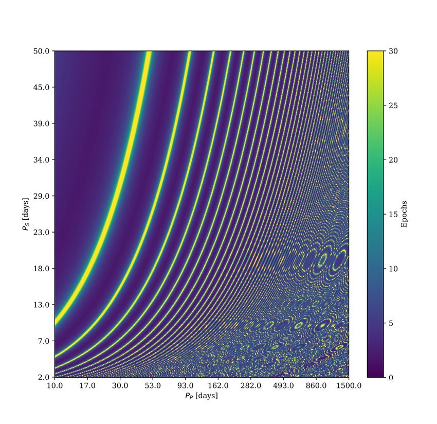
8 A. Teachey

 Number of moons 1 2 3 4 5
 Total (fixed host) 14819 5157 11612 10028 8384
 Total (%) stable 14793 (99.8%) 4752 (92.1%) 2694 (23.2%) 739 (7.4%) 161 (1.9%)
 + ΔBIC ≤ −2 12300 (83.0%) 3834 (74.3%) 1986 (17.1%) 448 (4.5%) 76 (0.9%)
 + cross-validated 11835 (79.9%) 3668 (71.1%) 1862 (16.0%) 414 (4.1%) 70 (0.8%)
 + ΔAIC ≤ 0 14033 (94.7%) 4527 (87.8%) 2460 (21.2%) 621 (6.2%) 121 (1.4%)
 + cross-validated 13433 (90.6%) 4311 (83.6%) 2311 (19.9%) 574 (5.7%) 112 (1.3%)
 TTV [epochs] 3.41+4.73
 −1.19
 3.38 +3.94
 −1.15
 +3.52
 3.25 −1.11 3.49 +2.56
 −1.48
 3.04 +3.71
 −0.99

 TTV [min] 1.84+11.38
 −1.37
 1.37 +6.85
 −0.97
 1.46 +10.22
 −1.0
 +15.27
 1.47 −0.99 0.70 +5.34
 −0.36
 Í
 ( ) / 5.5+3.1 × 10⁻³ 5.5 +3.2 × 10⁻³ 3.9 +3.7 × 10⁻³ 2.7 +3.6 × 10⁻³ +31.9 × 10⁻⁴
 6.7 −5.5
 −3.3 3.3 −2.6 −2.1

 Total (variable host) 15421 5148 11596 9486 7773
 Total (%) stable 15392 (99.8%) 4732 (91.9%) 2549 (22.0%) 550 (5.8%) 149 (1.9%)
 + ΔBIC ≤ −2 6418 (41.6%) 1905 (37.0%) 880 (7.6%) 173 (1.8%) 34 (0.4%)
 + cross-validated 6217 (39.9%) 1856 (35.6%) 827 (7.0%) 158 (1.6%) 34 (0.4%)
 + ΔAIC ≤ 0 12489 (80.1%) 3812 (73.1%) 1788 (15.2%) 333 (3.5%) 87 (1.1%)
 + cross-validated 11803 (75.7%) 3619 (69.4%) 1666 (14.2%) 299 (3.1%) 83 (1.1%)
 TTV [epochs] 3.44 +4.21
 −1.15
 3.42 +4.06
 −1.17
 +3.13
 3.24 −0.98 3.3 +2.16
 −0.89
 3.73 +3.61
 −1.36

 TTV [min] 2.96 +5.87
 −2.02
 2.65 +5.14
 −1.79
 2.8 +5.06
 −1.87
 2.6 +5.34
 −1.71
 2.37 +7.69
 −1.86
 Í
 ( ) / 5.6 +3.1 × 10⁻³ +3.2 × 10⁻³
 5.5 −3.5 3.3 +4.2 × 10⁻³ 1.5 +4.6 × 10⁻³ +9.7 × 10⁻⁴
 4.4 −3.7
 −3.5 −2.6 −1.2

 Total (resonant chain) 15012 4839 12522 10251 7376
 Total (%) stable 14983 (99.8%) 4381 (90.5%) 1429 (11.4%) 455 (4.4%) 168 (2.3%)
 + ΔBIC ≤ −2 6125 (40.8%) 1529 (31.6%) 460 (3.7%) 127 (1.2%) 41 (0.6%)
 + cross-validated 5833 (38.9%) 1471 (30.4%) 446 (3.6%) 125 (1.2%) 39 (0.5%)
 + ΔAIC ≤ 0 12130 (80.8%) 3434 (71.0%) 1059 (8.5%) 301 (2.9%) 100 (1.4%)
 + cross-validated 11475 (76.4%) 3256 (67.3%) 1006 (8.0%) 284 (2.8%) 94 (1.3%)
 TTV [epochs] 3.42 +3.98
 −1.15
 3.45 +4.65
 −1.17
 +3.61
 3.49 −1.21 3.43 +3.71
 −1.23
 4.05 +2.26
 −1.41

 TTV [min] 2.91 +6.1
 −1.99
 2.38 +4.78
 −1.63
 +4.1
 2.11 −1.45 2.32 +4.61
 −1.62
 2.01 +5.17
 −1.51
 Í
 ( ) / 5.5 +3.2 × 10⁻³ +3.0 × 10⁻³
 5.5 −3.7 2.6 +2.7 × 10⁻³ 1.5 +3.4 × 10⁻³ +27.9 × 10⁻⁴
 7.0 −5.2
 −3.4 −2.1 −1.3

Table 1. Summary of the “fixed host” (top five rows) and “variable host” (middle five rows) and “resonant chain” (bottom five rows) simulations produced for
this work. Percentages quoted indicate the fraction of total generated systems. Values quoted for TTV , TTV , and total satellite mass ratios are the median and
1 values for the robust cross-validation sample using ΔBIC as the selection metric.

useful metric, because it is safe to assume nature will not be making average required to be significantly lower in order to remain stable.
moons that are unstable on extremely short timescales. In other AT = 5, less than 2% of the generated systems were predicted to
words, their configurations will of course not be random. Systems be long-term stable.
that can survive O (104 ) orbits on the other hand are at least plausibly We point out that = 2 systems show the same median mass
formed by nature, even if they are eventually lost. ratio as = 1 systems (see Table 1), which at first glance might
 Figure 5 shows the survivability of the moon systems simu- be in tension with the trend just observed. This remains consistent
lated to completion as a function of total satellite system mass and however in view of the fact that we have opted to curtail the mass
architecture. For = 1 moon systems, they are virtually always sta- ratios of the satellite systems at 10−2 . Considered in isolation, = 1
ble; with no external perturbation, only strong tidal forces at small satellite systems could be stable up to a mass ratio approaching unity
moon semimajor axes may disrupt these systems on the timescale (a binary system). By contrast, we do not expect = 2 systems
of the simulation. Nevertheless about 0.2% of these systems are generally to be stable in that mass ratio regime. So there must be
eventually categorized as long-term unstable owing to a MEGNO some mass ratio at which = 2 systems are majority unstable,
number outside the established boundaries. Of course, more realistic consistent with the trend visible in Figure 5. Evidently that limit
simulations of single-moon systems, including the effects of stellar is above the mass ratio range we have explored here. Because for
perturbation and moon inclinations, would reveal a non-spherical = 1 and = 2 systems we have only probed the parameter space
region of stability, but for our purposes (initializing all moon orbits where stability is basically uniform across the entire range, it is not
 surprising that the median value for S / P , around 5 × 10⁻³ ,
 Í
as co-planar) this serves as a useful baseline of comparison.
 Once we get to > 1 moons, a trend becomes apparent: the is half that of the maximum value.
fraction of initialized systems predicted to be stable falls off steeply Figure 6 shows the distribution of period ratios for all three
as we increase , and notably, the total mass of these systems is on runs between all moon pairs. Slight deficits are evident around the

 MNRAS 000, 1–19 (2020)
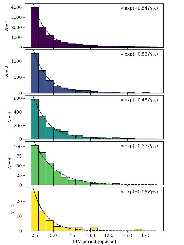
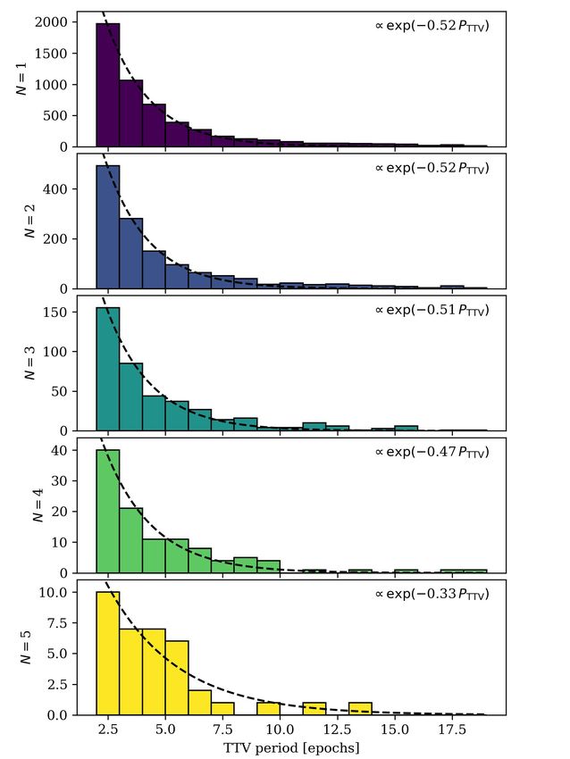
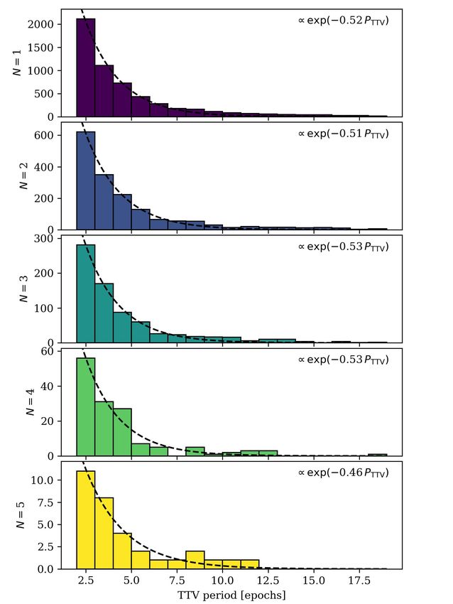
Generalized Exomoon Corridor 9
resonances in both the fixed host and variable host runs, but of curve in between. Applying the geometric observational bias yields
course the resonant chain run is comprised chiefly of moon pairs at virtually the same distribution as is shown here but suffers from a
these period ratios. reduction in the number of systems available and is thus less clean.
 We note also a reduction in the percentage of stable = 3
systems, by a factor of about 2, from the non-resonant to the resonant
architectures. The cause of this is not obvious, and in utilizing
a machine learning regressor with 10 inputs, a single culprit (for 5 ANALYSIS
example, eccentricity growth) is not readily identifiable. No such 5.1 Comparing the three simulation samples
reduction is apparent for the = 4 and = 5 systems, but this
could be because resonance is no longer the filtering factor. As more In this work we have compared three different simulation runs: one
moons are added, the moons are inherently more tightly packed, with a restricted host system architecture (consisting of a Solar-
and finer tuning is required for stability. Hence, these stringent analog star, Jupiter-analog planet, and a fixed photometric uncer-
requirements for stability may be equally met in both resonant and tainty), a second employing a realistic distribution of physical and
non-resonant architectures. observational attributes, and the last initializing all moon systems
 as resonant chains. Results from these runs are recorded in Table 1.
 There is a great deal of consistency between the three sets
4.2 Detectability of simulations. During the generation process we see quite similar
 numbers in terms of how many systems of each architecture survived
We turn now to examining the detectability of these signals. Figure random initialization. In particular, we note that all three = 2
7 indicates that the peak of each distribution falls right around systems had a survival rate roughly half that of > 2 systems,
Δ BIC = 0, but there are significant tails for these distributions in the suggesting that these systems are particularly prone to instability. We
fixed host systems, which can be responsible for pulling the median stress again that a careful interpretation is needed here; randomized
values well off the peak, especially for small systems. This tail = 2 systems are more unstable than the others, so the orbits of
is absent for the variable host and resonant chain systems, however. = 2 systems found in nature are unlikely to be “random”.
For the sample shown here we have implemented an additional, Likewise the total satellite mass ratios, falling off with increas-
observational bias such that simulated planets are represented in ing , follow the same trend across all three simulation runs. And
proportion to their geometric transit probability. We have assumed we see that both the derived median TTV and TTV values are
any transiting planet is equally likely to be discovered, however; broadly similar across all three runs, as well as consistent across
completeness is not a function of orbital period here. all choices for . This is a very important result, because it means
 We can see that as increases, there will be fewer and fewer the exomoon corridor result holds regardless of the assumptions we
such systems displaying strong evidence for TTVs based on the build into our model. Whether the moons sit in resonant chains or
ΔBIC metric. The systems also never display a more positive ΔBIC not, the measured TTV periods will pile-up at the short end.
than about 10, across all architectures, suggesting that this is what However, some important differences are evident. The total
would be needed to strongly rule out the presence of TTVs based number of systems that show evidence for a TTV as measured by
on our methodology. the ΔBIC falls off precipitously from the fixed host to the variable
 Figure 8 offers a glimpse into what is happening here. As host and resonant chain runs. This suggests than an occurrence rate
previously discussed, systems with fewer moons are in general more for exomoons based on a dynamical test such as this, if such a rate
stable at higher mass ratios (taking their simulation survival rates as can be derived, may be impacted by physical and observational
a proxy for stability). This in turn makes these systems on average system attributes. The situation is confusing, however, as the ΔAIC
more detectable, since a higher mass ratio corresponds to larger metric does not display this same drop-off. This could be because our
amplitude TTVs. adopted thresholds for ΔBIC and ΔAIC are not strictly compatible.
 Interestingly, the fixed host and variable host runs, where moon
 period ratios could take any value, show clear deficits at the 2:1
4.3 Exomoon corridor and 3:1 period ratios (Figure 6), in keeping with expectations that
At the crux of this investigation is the question of whether the resonances may contribute to instability. By contrast, the resonant
exomoon corridor finding – the pile-up of short TTV values – chain simulations have peaks at these period ratios, but that is merely
holds for ≥ 1 moons. Figure 9 demonstrates the distribution of an artefact of the methodology for generating the moons for this run.
measured TTV periods for the various moon architectures simulated It is encouraging to see that the majority of systems for which
in this work. ΔBIC ≤ −2 also cleared the cross-validation test. This suggests that
 We see that the exomoon corridor result does indeed generalize we are not imposing a significant additional bias in terms of the
for ≥ 1 moons, and evidently this characteristic distribution of systems we examine; by and large a system with a detectable TTV
TTVs is insensitive to the number of moons in the system, show- will also maintain the best period solution even as data are stripped
ing remarkable consistency. Each system represented here has a away.
ΔBIC ≤ −2 in favor of TTVs over linear ephemeris, and survived
our cross-validation test to ensure the period solutions are reliable.
The short-period pile-up also occurs without the cross-validation 5.2 Stability, Detectability, and Limitations
cut, but it is important to screen out those systems with inconsistent
 5.2.1 implications for detectable systems
period solutions to ensure that this is not merely a side-effect of
our methodology. We also screen out systems for which the TTV As we have discussed, the simulation results (Figure 5) across all
period solution is precisely equal to 2, as these solutions are gener- three simulations indicate a trend towards lower satellite system
ally spurious, placing every epoch at either the beginning or end of masses as we increase the number of moons. Multi-moon systems
the phase-folded solution and leaving a completely unconstrained with higher masses can of course exist in nature – assuming they

MNRAS 000, 1–19 (2020)

10 A. Teachey

 fixed host variable host resonant chain

 fraction stable
 # moons

 log10 ( Σ Ms / M P ) log10 ( Σ Ms / M P ) log10 ( Σ Ms / M P )

Figure 5. The fraction of stable systems for each architecture as a function of total satellite system mass in the fixed host (left), variable host (center), and
resonant chain runs (right).
 2:1

 3:1
 3:2

 5:2

 7:2

 4:1
 4:3
 5:4
 fixed host

 2:1

 3:1
 3:2

 5:2

 7:2

 4:1
 4:3
 5:4
 variable host

 2:1

 3:1
 3:2

 5:2

 7:2

 4:1
 4:3
 5:4
 resonant chain

 P outer / P inner P outer / P inner

Figure 6. Left: Distribution of period ratios in the fixed host, variable host, and resonant chain simulations (detail). All moon pairs are included, not just
adjacent pairs. Right: the same as before but zoomed out to reveal more structure, though still with a truncated -axis.

 MNRAS 000, 1–19 (2020)
Generalized Exomoon Corridor 11

 fixed host variable host resonant chain
 N=1

 N=1

 N=1
 fixed host variable host
 N=2

 N=2

 N=2
 N=3

 N=3

 N=3
 N=4

 N=4

 N=4
 N=5

 N=5

 N=5
 ΔBIC ΔBIC ΔBIC

Figure 7. Distribution of ΔBIC values for each architecture, for fixed host (left), variable host (center), and resonant chain (right) simulations. Representation
in this sample is weighted by geometric transit probability. The red dashed line in each plot shows the median value of the distribution. The long distribution
tails in the fixed host case are not shown.

 fixed host variable host resonant chain
ΔBIC

 ΔBIC

 ΔBIC

 Σ MS / M P Σ MS / M P Σ MS / M P

Figure 8. ΔBIC as a function of total moon mass for the fixed host (left), variable host (center), and resonant chain (right) simulations, color-coded by the
number of moons in the system. Our threshold for significance (-2) is indicated as a red dashed line.

can be formed in the first place – but they will be comparatively ratio limit of ∼ 10−4 based on simulations of moon accretion. At
rare, or they will have to be more finely tuned in order to survive. = 5, less than 2% of the generated systems were predicted to be
 long-term stable. More recent work on circumplanetary disk (CPD)
 Perhaps noteworthy is the fact that at = 4, system archi- evolution and moon production (e.g. Inderbitzi et al. 2020; Cilibrasi
tectures become majority unstable when total satellite system mass et al. 2020) have similarly predicted generally lower mass satellite
ratios go much above 10−4 – coincidental or not, this is in keep-
ing with the result from Canup & Ward 2006, who found a mass

MNRAS 000, 1–19 (2020)
12 A. Teachey

 fixed host variable host resonant chain
N=1

 N=1

 N=1
 fixed host
N=2

 N=2

 N=2
N=3

 N=3

 N=3
N=4

 N=4

 N=4
 N=5

 N=5

 N=5
 TTV period [epochs] TTV period [epochs] TTV period [epochs]

Figure 9. Distribution of inferred TTV periods for 1 < < 5 moon systems for the fixed host (left), variable host (center), and resonant chain (right)
simulations. Results were similar when a geometric observational bias is applied, but suffer from smaller numbers in each group. These results demonstrate
that the characteristic exomoon corridor distribution holds for > 1.

systems, which will in many cases be below our current dynamical sense that both predict we will not find many high mass, multi-moon
detection limits. systems. As such, we do not have to rely entirely on the predictions
 We caution the reader against over-interpreting the present of the CPDs to infer the relative probabilities of high-mass multi-
results; in particular, these stability fractions should not be read moon systems: even if the CPDs could produce them, the present
off as absolute occurrence rate probabilities or priors. Their initial analysis of post-CPD behavior suggests they will not be long-lived.
configurations (number, distribution, and masses) are not dictated To avoid this, the CPDs would have to be capable of fine-tuning the
by CPD models; depending on the density profile of the disks, there orbits.
may be more or fewer long-term stable moons produced in nature If we accept that satellite systems with more moons will gen-
than what we produce here by virtue of a different initial distribution erally have lower masses, as the present results suggest, this points
of moons. At the same time, it is worth keeping in mind that, due to to a possibly important observational bias in detecting exomoons.
the present dearth of exomoon system observations, CPD modeling Namely, we will be more likely to see systems with fewer moons,
has primarily (understandably) focused on explaining the regular by virtue of the fact that they permit substantially higher mass ra-
moons of our Solar System (e.g. Canup & Ward 2006; Szulágyi, tios, and these higher mass ratios generally correspond to larger
Cilibrasi, & Mayer 2018; Fujii & Ogihara 2020), and therefore amplitude TTVs.
might conceivably reflect an observational bias in that regard. If CPDs are incapable of producing mass ratios in excess of a
 Of course, moons are not only formed in CPDs; they may also few times 10−4 , we will then be biased towards identifying systems
be formed through impact scenarios (e.g. Canup & Asphaug 2001; for which this was not the formation pathway; capture or giant
Canup 2005; Ida et al. 2020) or capture scenarios (e.g. Agnor & impacts will be the more likely explanation for these massive moons,
Hamilton 2006; Nesvorný, Vokrouhlický, & Morbidelli 2007), for and if the Solar System is any guide, these moons will either be alone
example. Generally, these formation events are typically expected (as with the case of our Moon), or they will dwarf their companion
to produce a single massive moon, with perhaps some much smaller moons in the system (as with Triton and Charon). It is of course
moons as well, as in the case of Neptune (Banfield & Murray 1992) not currently known how likely these scenarios are in exoplanetary
and Pluto (Canup 2011). Still, it is at least conceivable that hereto- systems; if these pathways are less common, exomoon detections
fore un(der)explored formation pathways give rise to systems unlike may be quite rare in the near term. In any case, great care will need to
any seen in the Solar System (Teachey & Kipping 2018; Hamers & be taken in interpreting the relative occurrence rates of these types
Portegies Zwart 2018; Hansen 2019). Thus, it is at least conceivable of satellite systems as a window into planetary system formation.
that we might find systems with more than one massive moon that Where will we find these moons? On the one hand, shorter
did not form in a CPD, and we wish to simulate such systems. If period planets will display more transits, and this is clearly ad-
they are stable, they could potentially be found in nature. So long as vantageous as we search for dynamical signatures: more transits
these systems are not vastly over-represented in the sample, and their mean more data points with which to work, and a clearer signal can
inclusion does not wildly skew our results, we can feel confident in emerge. On the other hand, longer period planets have their own ad-
having them included. vantages. They will generally have longer transit durations, which
 Though our simulations are not produced from CPD profiles, boosts the timing precision (though this is a weak effect, as the tran-
 √
they are broadly consistent with the output of CPD models in the sit SNR only scales with in-transit data points). Moreover, as we

 MNRAS 000, 1–19 (2020)
You can also read