Projected changes of snow conditions and avalanche activity in a warming climate: the French Alps over the 2020-2050 and 2070-2100 periods
←
→
Page content transcription
If your browser does not render page correctly, please read the page content below
The Cryosphere, 8, 1673–1697, 2014
www.the-cryosphere.net/8/1673/2014/
doi:10.5194/tc-8-1673-2014
© Author(s) 2014. CC Attribution 3.0 License.

Projected changes of snow conditions and avalanche activity in a
warming climate: the French Alps over the 2020–2050 and
2070–2100 periods
H. Castebrunet1,2,3 , N. Eckert2 , G. Giraud3 , Y. Durand3 , and S. Morin3
1 INSA de Lyon, Laboratoire LGCIE, 20 Avenue des Arts, Bât. J.C.A. Coulomb, 69621 Villeurbanne, France
2 UR ETGR, IRSTEA/Université de Grenoble Alpes, BP 76, 38402 Saint Martin d’Hères, France
3 Météo-France – CNRS, CNRM-GAME UMR 3589, Centre d’Etudes de la Neige, 1441 rue de la Piscine,

38400 Saint Martin d’Hères, France

Correspondence to: H. Castebrunet (helene.castebrunet@insa-lyon.fr)

Received: 25 November 2013 – Published in The Cryosphere Discuss.: 23 January 2014
Revised: 11 July 2014 – Accepted: 17 July 2014 – Published: 15 September 2014

Abstract. Projecting changes in snow cover due to climate         projected to appear at high elevations earlier in the season.
warming is important for many societal issues, including the      At the same altitude, the southern French Alps will not be
adaptation of avalanche risk mitigation strategies. Efficient     significantly more affected than the northern French Alps,
modelling of future snow cover requires high resolution to        which means that the snowpack will be preserved for longer
properly resolve the topography. Here, we introduce results       in the southern massifs which are higher on average.
obtained through statistical downscaling techniques allow-           Regarding avalanche activity, a general decrease in mean
ing simulations of future snowpack conditions including me-       (20–30 %) and interannual variability is projected. These
chanical stability estimates for the mid and late 21st cen-       changes are relatively strong compared to changes in snow
tury in the French Alps under three climate change scenar-        and meteorological variables. The decrease is amplified
ios. Refined statistical descriptions of snowpack character-      in spring and at low altitude. In contrast, an increase in
istics are provided in comparison to a 1960–1990 reference        avalanche activity is expected in winter at high altitude be-
period, including latitudinal, altitudinal and seasonal gradi-    cause of conditions favourable to wet-snow avalanches ear-
ents. These results are then used to feed a statistical model     lier in the season. Comparison with the outputs of the deter-
relating avalanche activity to snow and meteorological condi-     ministic avalanche hazard model MEPRA (Modèle Expert
tions, so as to produce the first projection on annual/seasonal   d’aide à la Prévision du Risque d’Avalanche) shows gener-
timescales of future natural avalanche activity based on past     ally consistent results but suggests that, even if the frequency
observations. The resulting statistical indicators are funda-     of winters with high avalanche activity is clearly projected to
mental for the mountain economy in terms of anticipation of       decrease, the decreasing trend may be less strong and smooth
changes.                                                          than suggested by the statistical analysis based on changes in
   Whereas precipitation is expected to remain quite station-     snowpack characteristics and their links to avalanches obser-
ary, temperature increase interacting with topography will        vations in the past. This important point for risk assessment
constrain the evolution of snow-related variables on all con-     pleads for further work focusing on shorter timescales. Fi-
sidered spatio-temporal scales and will, in particular, lead      nally, the small differences between different climate change
to a reduction of the dry snowpack and an increase of the         scenarios show the robustness of the predicted avalanche ac-
wet snowpack. Overall, compared to the reference period,          tivity changes.
changes are strong for the end of the 21st century, but al-
ready significant for the mid century. Changes in winter are
less important than in spring, but wet-snow conditions are

Published by Copernicus Publications on behalf of the European Geosciences Union.
1674           H. Castebrunet et al.: Projected changes of snow conditions and avalanche activity in a warming climate

1   Introduction                                                   tion of the projected changes. In addition to intuitive conse-
                                                                   quences of warming such as wetting and a strong decrease of
In temperate mountainous areas, snow is a major component          snow cover area and height, these simulations suggest other
of the water cycle. As an important element of the critical        important effects, such as an increase of heavy snowfall at
zone at the interface between atmosphere, geosphere, ecosys-       high altitude or a much narrower snowmelt discharge peak in
tems and human societies, it has key impacts on geomorpho-         spring. However, great difficulties still remain, meaning that
logical processes, biodiversity and the tourism industry. As       prognoses regarding snow evolution are still debated (Räisä-
a consequence, since high-altitude (3000 m and more) areas         nen, 2008); the main obstacle in many impact studies per-
have been shown to be highly sensitive to climate change           tains to the robustness of the downscaling and debiasing of
(Beniston, 2003), understanding the responses of the snow-         large-scale atmospheric variables from regional or global cli-
pack to the ongoing warming, related impacts and poten-            mate models (GCM) to the mountain environment, featuring
tial feedbacks (e.g. albedo change) is of major environmen-        complex topography and, in particular, a wider altitude range
tal (e.g. Keller et al., 2005) and economic (e.g. Elsasser and     than in the topography resolved in GCMs (Rousselot et al.,
Buerki, 2002; Gonseth, 2013) interest. This can be achieved        2012; Bavay et al., 2009, 2013; Lafaysse et al., 2014; Ste-
by studying links between climate and snow cover for present       ger et al., 2013). To evaluate the potential impact of global
conditions, which includes an assessment of changes already        change on snow conditions in the French Alps for the forth-
measurable using various observation series, and by quanti-        coming decades through numerical simulations on relevant
fying changes to be expected in the future, using snow and         spatial scales, Rousselot et al. (2012) have developed statis-
regional climate simulations fed by global climate change          tical adaptation techniques. Specifically, an analogue method
scenarios.                                                         has been applied to regional climate model predictors so as
   Recent climate change in mountainous areas is now fairly        to provide complete, physically consistent time series of me-
well documented, for instance in the European Alps (e.g.           teorological variables which are needed for physically based
Beniston et al., 1997). Even if it has not been constant,          snowpack modelling.
with periods of slow temperature increase or even cooling,            Among the geomorphic processes controlled by snow and
the warming since the end of the Little Ice Age (∼ 1850)           meteorological variables, and, on longer timescales, by cli-
has been marked and accelerated over the 1985–2000 pe-             mate, natural avalanche activity strongly impacts mountain
riod (e.g. Beniston, 2005b). Following studies on larger spa-      communities through the related risk for humans and in-
tial scales (e.g. Brown, 2000; Mote, 2003; Huntington et al.,      frastructures. Hence, the possible occurrence of catastrophic
2004; McCabe and Wolock, 2010), several studies have doc-          events (e.g. Ammann and Bebi, 2000) under ongoing climate
umented decreases in snow precipitation, snow depths, snow         change requires accurate adaptation strategies (Richard et al.,
cover durations or snow water equivalent in many countries         2010). However, how to quantify the impact of the recent
of the Alpine region (e.g. Falarz, 2002, 2004; Laternser and       changes in mountain climate on natural avalanche activity
Schneebeli, 2003; ONERC, 2008; Valt and Cianfarra, 2010;           and its future evolution in terms of possible modifications
Serquet et al., 2011; Marty and Meister, 2012). Increased          of the frequency and intensity of both ordinary and extreme
variability has also been observed, especially for winter tem-     events remains a rather open question (Keiler et al., 2010;
peratures, inducing an increasing number of warm winter            IPCC, 2012).
spells (Beniston, 2005a). Lastly, efforts have been made to           Evidence of significant changes in real avalanche data se-
quantify elevation-dependent effects on warming (Rangwala          ries over the last 60 years has been provided over the last
and Miller, 2012) and their complex interaction with the           years, notably in the French Alps (Eckert et al., 2010a, b,
freezing level, leading to less marked trends in snowpack          2013), with clear links to snow and meteorological changes
depth and duration at high altitude (Moran-Tejeda et al.,          (Castebrunet et al., 2012) and their altitudinal control (Lav-
2013). For the specific case of the French Alps, a fairly com-     igne et al., 2012, 2014). The question of observed changes
plete picture of recent changes is available, including sub-       in different types of avalanche activity (wet/dry and or
regional, altitudinal and seasonal gradients, thanks to system-    with/without a powder component) has been tackled even
atic point measurement analysis (Dumas, 2012) and snow-            more recently (Pielmeier et al., 2013; Eckert et al., 2013).
pack and meteorological reanalyses (Durand et al., 2009a,          Regarding future evolution for the 21st century, to our
b).                                                                knowledge, the only existing results are those of Martin et
   Concerning future snowpack evolution, first estimations         al. (2001) and Lazar and Williams (2008). These studies both
have been obtained through simple extrapolations of cur-           suggested an ongoing increase in the proportion of wet-snow
rent observed trends (e.g. Beniston et al., 2003) or sensitivity   avalanches as compared to dry-snow avalanches, and a shift
studies using snowpack models (Martin et al., 1994). More          in their timing. This is consistent with already existing field
detailed future simulations of the snow cover using climate        observations of snow cover wetting on a small scale and
change scenarios as input have emerged recently (e.g. Lopez        its link with wet-snow release susceptibility (Mitterer et al.,
Moreno et al., 2009, 2011; Bavay et al., 2009, 2013; Lafaysse      2011), but without a clear quantification of how this corre-
et al., 2014; Piazza et al., 2014), allowing better quantifica-    lates to the amplitude of change in total avalanche activity.

The Cryosphere, 8, 1673–1697, 2014                                                      www.the-cryosphere.net/8/1673/2014/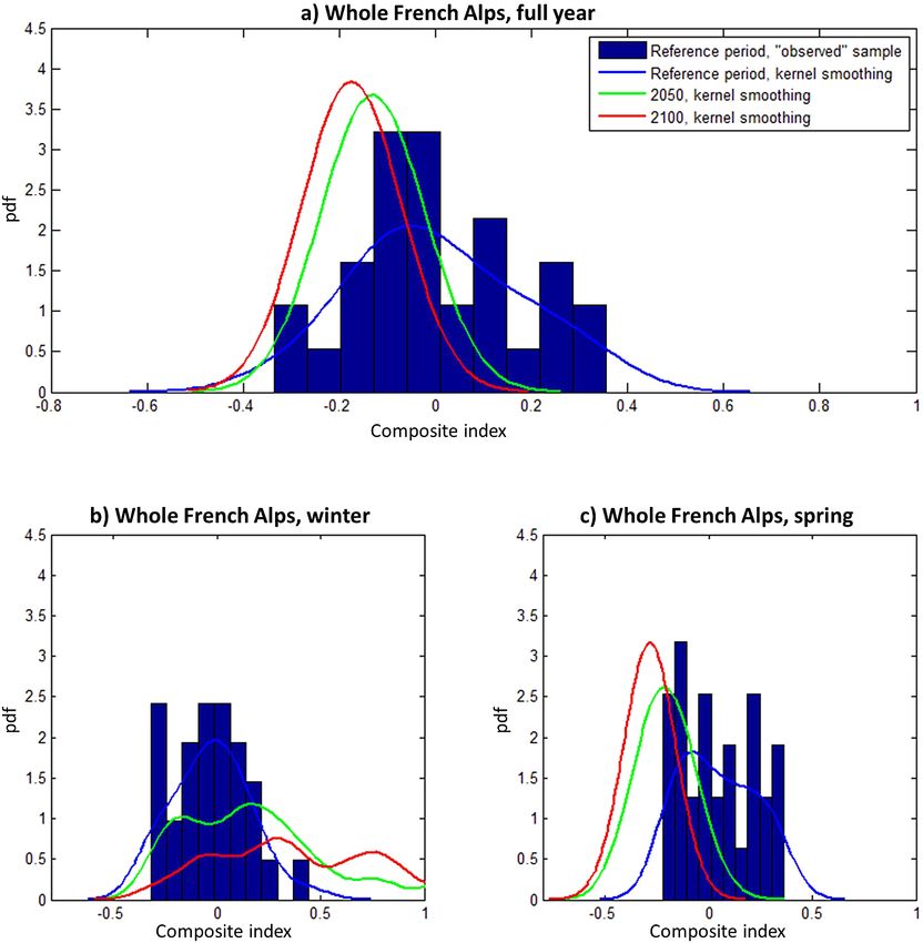
H. Castebrunet et al.: Projected changes of snow conditions and avalanche activity in a warming climate 1675
On the basis of these works, the current study aims at pro-
ducing a detailed description of projected changes of snow-
pack characteristics expected in the French Alps in the mid
and late 21st century, including latitudinal, altitudinal and
seasonal gradients and under three greenhouse gas (GHG)
emissions scenarios. These results, expanding on those of
Rousselot et al. (2012), are then used to feed statistical mod-
els developed by Castebrunet et al. (2012) to link avalanche
activity and the snow and meteorological data produced by
the SAFRAN–Crocus–MEPRA (Système d’Analyse Four-
nissant des Renseignements Adaptés à la Nivologie–Crocus–
Modèle Expert d’aide à la Prévision du Risque d’Avalanche)
model chain (see below). Hence, future changes in avalanche
activity on annual/seasonal timescales are compared to the
1960–1990 control period on the basis of natural, actually
observed avalanche activity and simple but robust statistical
relations.
2 Data and methods
2.1 Past meteorological, snow and avalanche data on
the massif scale
The primary data used in this study consists of daily ob-
served and simulated past snow and meteorological data and
avalanche counts over the French Alps on the geographical
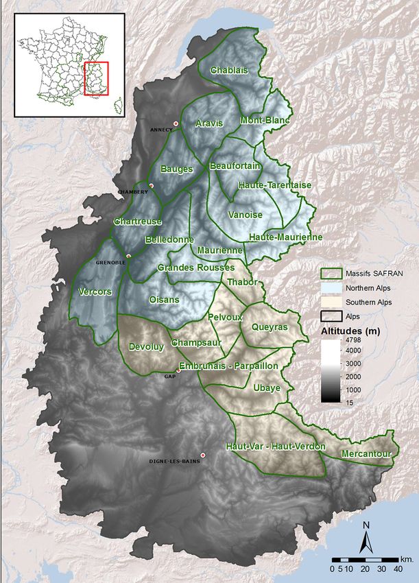
scale of the 23 massifs of the French Alps used for opera- Figure 1. Area studied. Within the SAFRAN model, the French
tional avalanche forecasting (Fig. 1). The surface area of each Alps are divided into 23 massifs (source: H. François, IRSTEA, In-
massif is about 500 km2 , and the key assumption regarding stitut de recherche en sciences et technologies pour l’environnement
snow and meteorological numerical simulations is their spa- et l’agriculture).
tial homogeneity, i.e. within each massif meteorological and
snowpack properties are assumed to depend only on altitude,
slope and aspect (Durand et al., 1999).
Daily observed avalanche data come from the “Enquête merous and detailed in previous studies (e.g. Eckert et al.,
Permanente sur les Avalanches” (EPA) which describes the 2010c; Castebrunet et al., 2012).
avalanche events on approximately 3900 designated paths In this study, among all the available information, only
in the French Alps and Pyrenees since the beginning of the avalanche counts, which represents the most natural variable
20st century (Mougin, 1922). The most common use for EPA to describe the frequency of the phenomenon, are considered.
data is hazard (e.g. Ancey et al., 2004; Eckert et al., 2007a) In this case, the predominant source of error to be consid-
and risk (e.g. Eckert et al., 2009) assessment on the path ered is unrecorded events. Locally, the quality of the records
scale. However, the EPA is also well suited for large-scale depends to a large extent on careful data recording by lo-
studies on relations with snow and meteorological covariates cal observers (mostly forestry rangers). However, once the
(Jomelli et al., 2007), major avalanche episodes (Eckert et avalanche counts are aggregated on the massif scale, these
al., 2010c) and spatial variations in avalanche activity (Eck- local heterogeneities are smoothed, making the automatic de-
ert et al., 2007b). For climate studies, the major advantages of tection of abnormally low records very difficult. For instance,
the EPA are the long time span of the available data series in there does not exist any local series which can be considered
the context of a well-structured observation network, giving a fully error-free with certainty. As a consequence, homoge-
relatively accurate view of the spatio-temporal fluctuations of nization methods (e.g. Caussinus and Mestre, 2004) are dif-
natural avalanche activity in France over the last century. Var- ficult to implement and were not used in this study. This must
ious quantitative (run out elevations, deposit volumes, etc.) be kept in mind when interpreting results. Also, it is gener-
and qualitative (flow regime, snow quality, etc.) data (Jamard ally admitted that the EPA record underestimates avalanche
et al., 2002) are recorded. Sources of uncertainties and sys- activity at high elevations because human observations con-
tematic errors in the estimation of certain variables are nu- cern mainly paths visible from valley floors. This is another
www.the-cryosphere.net/8/1673/2014/ The Cryosphere, 8, 1673–1697, 2014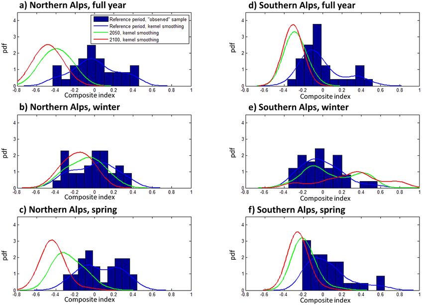
1676           H. Castebrunet et al.: Projected changes of snow conditions and avalanche activity in a warming climate

potential source of bias to be addressed while exploiting the           thus captured in our definition of recent surface dry
extremely valuable information conveyed by EPA records.                 snow.
   Daily snow and meteorological conditions consist of out-
puts from a reanalysis of meteorological and snow condi-           – The MEPRA natural snowpack instability index, which
tions computed using the SAFRAN–Crocus–MEPRA model                   is a proxy for avalanche hazard (Giraud, 1993; Durand
chain (SCM; Durand et al., 1999, 2009a, b). The meteo-               et al., 1999), is a diagnostic tool assessing snowpack
rological analysis is performed on the scale of the massifs          stability based on Crocus-simulated snow stratigraphy.
shown in Fig. 1, for which meteorological conditions are as-         MEPRA outputs, which are computed within each mas-
sumed to be homogeneous but to vary with altitude. Durand            sif for each slope, altitude and aspect class, are aggre-
et al. (2009a, b) performed a complete reanalysis of mete-           gated on the massif scale, thereby providing a single
orological and snow conditions with SCM using 44 years               scalar value for a given date. This aggregated MEPRA
of analysed large-scale atmospheric model data from the              index, called hereafter MI, varies between 0 and 8 (8
40-year European Centre for Medium-Range Weather Fore-               being the higher instability level) dependent on both
cast (ECMWF) reanalysis (ERA-40) project (Uppala et al.,             the SAFRAN–Crocus inputs and the characteristics of
2004), together with meteorological observations including           each massif. The MI should be viewed as a synthetic
numerous mountain stations. This reanalysis, complemented            combination of SAFRAN–Crocus snow and meteoro-
for several years beyond the end date of the ERA-40 data set         logical data relevant to estimate potential avalanche re-
using large-scale meteorological fields from Météo-France            lease rather than a true measure of avalanche activity.
operational numerical weather prediction models, covers the          It is important to keep in mind that the MI is used in
period from 1958 to 2009 and is referred to as the model run.        an operational context to help the forecasting of po-
For the present study, the variables given below were used,          tential snowpack instability and so has to be sensitive
similar to those described by Castebrunet et al. (2012). They        to snow and meteorological conditions especially when
concern the 23 alpine massifs (Fig. 1) for three elevations          avalanche hazard is important. On the other hand, this
(low, mid and high – 1800, 2400, and 3000 m a.s.l.), leading         index is less sensitive in the case of instability being
to 57 variables in total:                                            lower, leading to sporadic events on the massif scale, as
                                                                     discussed in Castebrunet et al. (2012).
  – Daily cumulated precipitation (rain and snow), tem-
    perature (daily minimum, maximum, and mean), max-            2.2    Relating avalanche activity to snowpack and
    imum daily wind speed and the associated direction                  meteorological covariates through regression
    (SAFRAN outputs).                                                   models on large spatio-temporal scales

                                                                 Castebrunet et al. (2012) proposed a time-implicit approach
  – For the four main aspects (northern, eastern, southern,
                                                                 for the detection of abnormal years and low-frequency trends
    and western) and 40◦ slope, the snow depth, the thick-
                                                                 in various indicators of natural avalanche occurrence: EPA
    ness of surface wet snow and the thickness of recent
                                                                 counts, MEPRA index and a composite index combining
    surface dry snow. These variables are derived from out-
                                                                 these two measures (see below). The best explanatory snow
    puts of the detailed snowpack model Crocus fed by
                                                                 and meteorological covariates were selected with a step-
    SAFRAN meteorological conditions (Brun et al., 1992).
                                                                 wise regression (e.g. Saporta, 2006), i.e. a variable selection
    The thickness of surface wet snow is defined, starting
                                                                 procedure for linear models in which the set of predictive
    from the top of the snowpack downwards, as the sum
                                                                 variables is retained by an automatic sequence of Fisher F
    of the vertical component of the thickness of the con-
                                                                 tests. The regression model obtained relates the series yt of
    tiguous wet-snow layers characterized by a liquid wa-
                                                                 avalanche activity indicators to P selected standardized ex-
    ter content greater than 0.5 % by volume. The thick-
                                                                 planatory variables Xjnorm
                                                                                         t  such that
    ness of the recent surface dry snow is defined as the
    vertical distance between the snowpack surface and the              p
    deepest snow layer characterized by a dendricity greater
                                                                        X
                                                                 yt =          Xjnorm
                                                                                  t βj + εt ,                               (1)
    than 0.25. The threshold expressed in terms of den-                 j =1
    dricity (Brun et al., 1992) ensures that the considered
    snow layer still features characteristics of precipitation   with βj , the weighting coefficient, representing the contribu-
    particles or decomposed fragments (Fierz et al., 2009),      tion of each predictive variable retained to the fluctuations
    and it accounts for the impact of snow metamorphism          of avalanche activity, and εt being the residual activity not
    on snow layers in a more consistent way than relying         predicted by the model. The values of εt are modelled as
    only on snow age because the rate of transformation of       independent and identically distributed realizations of a cen-
    snow properties strongly depends on temperature, tem-        tred Gaussian random number with standard deviation σ . The
                                                                             p
    perature gradient and the occurrence of wet-snow con-        function
                                                                            P
                                                                               Xjnorm
                                                                                  t βj , seen as a time series, shows temporal
    ditions, which are explicitly considered in Crocus and                     j =1

The Cryosphere, 8, 1673–1697, 2014                                                        www.the-cryosphere.net/8/1673/2014/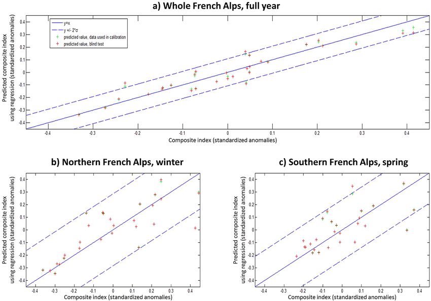
H. Castebrunet et al.: Projected changes of snow conditions and avalanche activity in a warming climate                       1677

fluctuations that are clearly related to the temporal fluctua-      of their daily values during the year/season:
tions of the covariates, hence providing a better understand-
ing of the response of avalanche activity to changes in its              1
                                                                    CIt = (0.5EPAnorm
                                                                                 t    + 0.5MEPRAnorm
                                                                                                t    + ρt ).                    (2)
most important drivers than a direct time series analysis of             3
the yt series.
   Rather than focusing on daily counts on the massif scale,        It gives equal weight to EPA counts and the MI and favours
Castebrunet et al. (2012) considered larger spatio-temporal         or disfavours years or seasons where both index are consis-
scales. Annual (15 December to 15 June) and seasonal (win-          tent or unconsistent, and vice versa. Standardization is used
ter and spring) series of anomalies were calculated both for        to spread the values over a [−2, 2] range similar to the one
the entire French Alps and for two sub-regions referred to          corresponding to the explanatory variables. Finally, while the
as the northern French Alp, and the southern French Alps            CI is primarily computed on the massif scale, obtaining spa-
(Fig. 1). Winter and spring seasons were defined as the             tially averaged time series is straightforward, assuming sim-
15 December to 14 March and 15 March to 15 June sub-                ilar weights for all massifs.
periods. On these scales, regression models between the                Based on this work, we assume in this study that the CI is
SCM–ERA40 outputs and avalanche activity cover the pe-              the best indicator of natural avalanche activity and we base
riod 1958–2009. Analysis and validation showed that they            the assessment of future changes in avalanche activity on it
were able to represent both high and low peaks and low-             for the same nine spatio-temporal scales (three regions and
frequency trends, indicating a clear statistical relation be-       three periods; see Sect. 3). We will, however, check and dis-
tween the fluctuations of avalanche activity and those of the       cuss the consistency of the patterns we highlight with the an-
selected covariates. This was a rather surprising result given      nual/seasonal changes using the MI, which can be computed
that the avalanche release process is a strongly discontinuous      for the future from the simulations of future snow charac-
response to meteorological patterns and changes in snow-            teristics, in contrast to EPA data, which by their nature are
pack characteristics, so that a weaker and/or nonlinear rela-       only available for past years. In addition to the work already
tion was expected for sub-seasonal and seasonal scales. It ap-      reported by Castebrunet et al. (2012), we developed new re-
peared that the explanation may be that averaging over large        gression models with the same stepwise selection methodol-
areas and relatively long periods smoothes the signal, switch-      ogy but considering only the period 1961–1990 (instead of
ing from meteorological and snowpack control on the daily           1958–2009) of the simulation SCM–ERA40. This was found
scale to seasonal characteristics of the latter, making it possi-   necessary for (i) dealing with the control period used for the
ble to capture the predominant factors for the long-term inter-     climate projections (see Sect. 2.3), and (ii) enlarging the tem-
annual evolution in a more climatological sense with simple         poral gap between the reference period 1961–1990 and the
statistical regression models. On the other hand, the approach      2020–2050 period.
loses the information related to the succession of short-term          The obtained nine new CI regression models are sum-
meteorological situations (e.g. multiday intense snowfall) in-      marized in Tables 1–3. All determination coefficients are
teracting with a few massifs, except from the perspective           very good (higher than 0.7), which illustrates the relevance
of their contribution to the annual/seasonal mean. Hence,           of explaining avalanche activity with a few (from one to
the approach is adapted to investigate seasons of high/low-         nine) snowpack and meteorological covariates. On the largest
avalanche activity over large areas but not for the more lo-        scale considered (the entire French Alps and the whole
calized 1–7-day episodes of highest activity. See Sect. 4 for       avalanche year, Table 1), the CI model (determination coef-
further discussion of spatio-temporal scales.                       ficient R 2 = 0.91) includes four snow variables, all of which
   Castebrunet et al. (2012) also showed that good correla-         relate to northern slopes. Only snow depth at 2400 m has a
tions exist between EPA avalanche counts and the MEPRA              negative contribution to the avalanche activity indicator CI.
index (MI) during cold winter periods even if the MI may            The statistical method employed indicates that more vari-
better represent such conditions due to avalanche counts            ables are required to explain the CI for the northern French
missed due to bad weather. In contrast, it was found that the       Alps (nine), while four are sufficient for the southern French
MI often fails to capture avalanche activity linked to wet-         Alps. This difference in variable numbers necessary to ex-
snow conditions during spring and, more generally, localized        plain the year-to-year variability of avalanche activity may
or short avalanche events. To limit these drawbacks/biases,         be linked to the larger extension of the northern French Alps,
a composite index referred to as CI was proposed to com-            which include three massifs characterized by low altitude
bine EPA and MI avalanche activity indicators and better            (under 2500 m), making the triggering contexts less homo-
represent the overall natural activity. It is computed using the    geneous. The retained variables in the northern French Alps
annual anomalies of the instability index MEPRAnorm     t    and    concern different slope orientations (north, east and west)
avalanche counts EPAnormt   , and the correlation  coefficient ρt   and maximal daily temperatures at mid and high elevations in
                                                                    addition to snowpack characteristics. For the southern French
                                                                    Alps, the CI model includes snow precipitation at 3000 m and
                                                                    snowpack variables for north and west slopes.

www.the-cryosphere.net/8/1673/2014/                                                        The Cryosphere, 8, 1673–1697, 2014
1678            H. Castebrunet et al.: Projected changes of snow conditions and avalanche activity in a warming climate

Table 1. Regression model characteristics for the French Alps (all year, winter and spring periods). For each model, the different variables
are those selected by the stepwise regression. For each retained normalized explanatory variable, Xjnorm
                                                                                                     t , βj is the corresponding weighting
coefficient in the model; ρj the correlation coefficient between Xjnorm                                  2
                                                                    t , βj and the composite index; and R the determination coefficient of
the model.

                                                             French Alps, year
                             Explanatory variables j                                      βj       ρj      R2
                             Snow precipitation (1800 m)                               0.09      0.84    0.91
                             Thickness of wet snow (1800 m, north)                     0.06      0.84
                             Snow depth (2400 m, north)                               −0.13     −0.70
                             Thickness of recent surface dry snow (3000 m, north)      0.12      0.89
                                                            French Alps, winter
                             Explanatory variables j                                      βj       ρj      R2
                             Thickness of wet snow (2400 m, north)                     0.09      0.23    0.82
                             Thickness of recent surface dry snow (3000 m, east)       0.34      0.85
                             Thickness of recent surface dry snow (2400 m, west)      −0.19     −0.80
                                                            French Alps, spring
                             Explanatory variables j                                      βj       ρj      R2
                             Thickness of wet snow (2400 m, north)                    −0.09      0.01    0.89
                             Thickness of wet snow (2400 m, east)                      0.16      0.53
                             Thickness of recent surface dry snow (3000 m, south)     −0.13     −0.73
                             Thickness of recent surface dry snow (2400 m, west)       0.26      0.81
                             Snow depth (3000 m, west)                                −0.07     −0.45

   Regarding the winter period, CI models for the three re-             year, which is then predicted with the fitted model. Figure 2
gions are characterized by a limited number of covariates               shows the predictive performance of three statistical models
related to thickness of snow (1 to 3) and by the predomi-               corresponding to the different regions/time periods studied.
nant contribution of the thickness of recent surface dry snow           Nearly all predicted values fall in the 95 % confidence inter-
at 3000 m for eastern slopes (marginal correlation with the             vals around the data (the traditional ± two standard devia-
composite index ρj > 0.8). This highlights that this season             tions in a linear regression), and predictions obtained with
is dominated by fresh dry-snow avalanches. While for the                this validation procedure are very close to the ones obtained
northern French Alps the statistical model only includes the            when the whole data set is used for calibration.
thickness of recent surface dry snow, the thickness of wet                 Table 4 quantifies and generalizes these statements, show-
snow for northern slopes also contributes to the statistical            ing that, for all the models, nearly “perfect” success rates are
models on the scales of both the entire French Alps and                 obtained in calibration, i.e. around 95 % of the predictions
southern French Alps.                                                   falling in the 95 % confidence intervals around the data. In
   For the spring period, more variables are required to ad-            the leave-one-out cross-validation procedure, success rates
equately explain the annual fluctuations of the CI (two to              are, unsurprisingly, a bit lower, but remain as high as ∼ 90 %,
five). They concern snowpack characteristics, mainly at mid             showing that in each region/period, the model is able to pre-
(2400 m) and high (3000 m) elevations. For instance, two of             dict correctly nearly all observations without the data corre-
four variables are thicknesses of wet snow for the northern             sponding to each observation. Again, the slightly lower pre-
French Alps, which is consistent with the fact that spring              diction rates for the northern French Alps (full year and win-
avalanches are mainly wet-snow avalanches. Notably, this is             ter) may be linked to their large extension and, hence, het-
not the case for the southern French Alps, but the snow depth           erogeneity. However, this may also be fortuitous, since the
on south-facing slopes is included in the model and may play            differences between prediction rates between zones/periods
a similar role.                                                         are quite small. Anyhow, these results can be considered very
   The efficiency and robustness of the nine regression mod-            satisfactory considering the crudeness of the statistical mod-
els have been evaluated and checked on the 30-year calibra-             elling approach employed. They give confidence in the fitted
tion sample using a leave-one-out validation scheme. In the             relationships between avalanche activity and meteorological
latter, each “data point” (year) is in turn removed from the            and snowpack conditions, and in their ability, despite their
calibration sample; the model is fitted without the removed             arguable oversimplification, to roughly reproduce different

The Cryosphere, 8, 1673–1697, 2014                                                             www.the-cryosphere.net/8/1673/2014/
H. Castebrunet et al.: Projected changes of snow conditions and avalanche activity in a warming climate                              1679

Table 2. Regression model characteristics for the northern French Alps (all year, winter and spring periods). For each retained explanatory
variable Xjnorm
            t , βj is the corresponding weighting coefficient in the model; ρj is the correlation coefficient between Xj t
                                                                                                                          norm , β and the
                                                                                                                                  j
composite index; and R 2 is the determination coefficient of the model.

                                                        Northern French Alps, year
                             Explanatory variables j                                     βj        ρj     R2
                             Tmax (2400 m)                                            −0.15     0.32     0.97
                             Tmax (3000 m)                                             0.19    −0.19
                             Thickness of wet snow (1800 m, north)                    −0.05    −0.85
                             Thickness of recent surface dry snow (1800 m, north)      0.43     0.87
                             Thickness of recent surface dry snow (3000 m, north)     −0.27    −0.90
                             Thickness of wet snow (2400 m, east)                      0.17     0.61
                             Thickness of recent surface dry snow (3000 m, east)       0.43     0.90
                             Thickness of recent surface dry snow (1800 m, west)      −0.34    −0.87
                             Thickness of wet snow (2400 m, west)                     −0.11    −0.50
                                                       Northern French Alps, winter
                             Explanatory variables j                                     βj        ρj     R2
                             Thickness of recent surface dry snow (3000 m, east)        0.22     0.85    0.71
                                                       Northern French Alps, spring
                             Explanatory variables j                                     βj        ρj     R2
                             Thickness of recent surface dry snow (2400 m, north)      0.35     0.78     0.80
                             Thickness of wet snow (2400 m, east)                      0.26     0.45
                             Thickness of wet snow (2400 m, west)                     −0.20    −0.33
                             Thickness of recent surface dry snow (3000 m, west)      −0.21    −0.72

types of avalanche episode contexts, at least for the climate               – The A2 scenario assumes regionally heterogeneous eco-
of the reference period (see Sect. 4 for discussion of their                  nomic and technological development throughout the
validity under a future climate).                                             world and a continuously increasing population. This is
                                                                              one of the most greenhouse-gas(GHG)-emissive IPCC
2.3 Modelling climate, snowpack characteristics and                           scenarios.
    avalanche activity in the future
                                                                            – The B1 scenario assumes similar evolution of the global
In order to carry out projections of the impact of climate                    population to that in A1B, but with an economy dom-
change on snow conditions and avalanche activity in the                       inated by services and information activities and the
French Alps, the model chain SCM was run using, as input,                     use of clean technologies. This scenario is the least-
a reanalysis of meteorological conditions spanning the pe-                    emissive one, with GHG emissions that are stabilized
riod 1960–1990 and synoptic-scale meteorological variables                    before the end of the century.
from the regional climate model (RCM) ALADIN-climate-
V4 (Aire Limitée Adaptation dynamique Développement In-                   Since A1B scenario is the closest to the 2050 forecasts of
terNational) (Rousselot et al., 2012), run at 12 km resolution.           the International Energy Agency, we mainly focus on this
   Three running periods have been considered: the reference              scenario in this work, but the three of them were tested and
period (1961–1990) and two future periods in the mid and                  the results are briefly reported in Sect. 3.
late 21st century (2021–2050 and 2071–2100) according to                     The ALADIN RCM boundary conditions were provided
three 4th IPCC (IPCC, 2007) emission scenarios (IPCC Spe-                 by the global ARPEGE-climate-V4 (Action de Recherche
cial Report on Emissions Scenarios (SRES) B1, A1B and                     Petite Échelle Grande Échelle) GCM (Deque and Somot,
A2):                                                                      2007), running with a variable horizontal resolution of about
                                                                          50 km over Europe. The sea surface temperature used for
  – The A1B scenario describes a future world with rapid,                 coupling ALADIN to ARPEGE originates from previous
    globalized economic growth, the development of new,                   coarser resolution runs of ARPEGE. The reference pe-
    more efficient technologies, and a global population in-              riod (called EM6) is a continuous ALADIN simulation be-
    crease until the mid century with a decline thereafter.               tween 1961 and 1990, whereas both future climatic periods,

www.the-cryosphere.net/8/1673/2014/                                                             The Cryosphere, 8, 1673–1697, 2014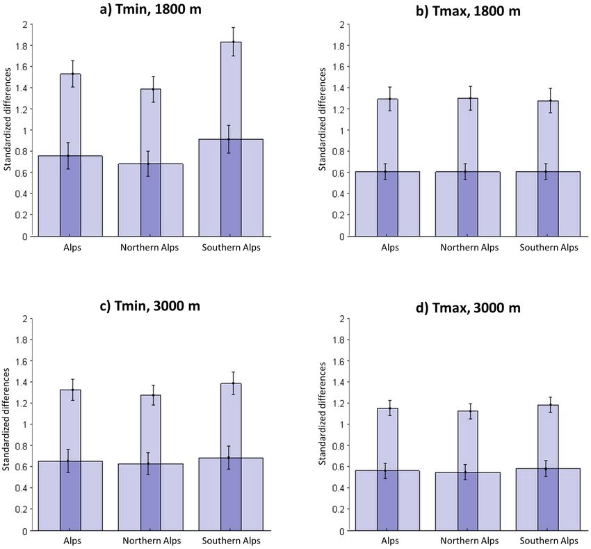
1680             H. Castebrunet et al.: Projected changes of snow conditions and avalanche activity in a warming climate

Figure 2. Cross-validation of the composite index regression model for the reference period: entire French Alps for the full avalanche year
(a), northern French Alps in the winter season (b) and southern French Alps in the spring season (c). In each panel, the predictive performance
is assessed with/without (leave-one-out scheme) each pseudo-observation. To represent predictive uncertainty around the first bisector, the
classical bandwidth of ± two standard deviations is included.

2021–2050 (called EM7) and 2071–2100 (called EM9), are                       Firstly, for each simulation and each ALADIN grid point,
simulations consisting of 30 independent yearly simulations.              meteorological daily fields are compared with daily data
   The method implemented here to compute the im-                         from the ECMWF ERA-40 reanalysis (Uppala et al., 2004),
pact of climate change on meteorological conditions in                    and a date with analogue weather conditions is identified
the SAFRAN massifs representing the French Alps de-                       through an appropriate distance. The series of analogue dates
rives from Rousselot et al. (2012) with significant differ-               is then used to extract corresponding meteorological data
ences. Indeed, Rousselot et al. (2012) carried out nearest-               from the SCM–ERA40 meteorological reanalysis (Durand et
neighbour research of similar meteorological situations (ana-             al., 2009a) that we call EMxCS  DATE , with x = 6, 7 or 9 and
logue method) from the synoptic-scale field output from AL-               CS being the SRES scenario, namely A1B, A2 or B1. Per-
ADIN for the present and future climate and associated it                 centiles of each meteorological variable for each scenario
with the corresponding meteorological forcing for each date               and time period are then computed based on each collec-
from the SAFRAN reanalysis (Durand et al., 2009a, b) to                   tion of SCM–ERA40 data for the corresponding selected
build the meteorological forcing data set (referred to as the             dates. Percentiles for the same variables but for the entire
DATE method). This method has the benefit of following                    SCM–ERA40 time series were also computed. For consis-
the large-scale chronology of meteorological conditions from              tency, the SCM–ERA40 data series used were limited to the
the ALADIN RCM, but it introduces discontinuities in me-                  1960–1990 period, both for the data search and for the per-
teorological variables every day between two analogue days.               centile calculation. These percentiles (at rank α) are denoted
                                                                                                           ERA40
In this study, an alternative approach was taken, fully rely-             as qα (EMxSC DATE ) and qα (SCM        ), respectively, and are
ing on the chronology of meteorological conditions from the               used to produce ranked differences, at the same α percentile
reference period 1960–1990 and applying corrections to this               value, between the different RCM projections (as a series of
continuous time series based on a quantile-mapping method                 dates) and the statistics of meteorological variables into the
(Deque, 2007).                                                            SCM–ERA40 record.

The Cryosphere, 8, 1673–1697, 2014                                                               www.the-cryosphere.net/8/1673/2014/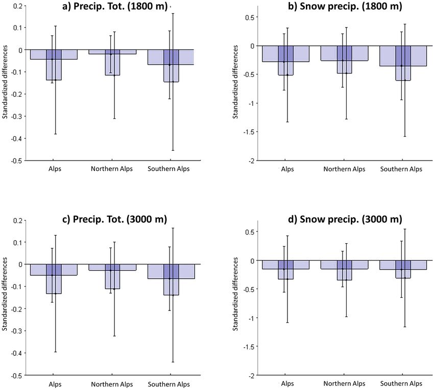
H. Castebrunet et al.: Projected changes of snow conditions and avalanche activity in a warming climate                                1681

Table 3. Regression model characteristics for the southern French Alps (all year, winter and spring periods). For each retained explanatory
variables Xjnorm                                                                                                           norm
             t , βj is the corresponding weighting coefficient in the model; ρj is the correlation coefficient between Xj t , βj and the
composite index; and R 2 is the determination coefficient of the model.

                                                           Southern French Alps, year
                              Explanatory variables j                                             βj       ρj      R2
                              Snow precipitation (3000 m)                                   −0.08       −0.55
                              Thickness of wet snow (1800 m, north)                          0.14        0.86
                                                                                                                  0.91
                              Snow depth (2400 m, north)                                    −0.09       −0.65
                              Thickness of recent surface dry snow (3000 m, west)            0.22        0.85
                                                        Southern French Alps, winter
                              Explanatory variables j                                             βj       ρj      R2
                              Thickness of wet snow (2400 m, north)                          0.11        0.23
                              Thickness of recent surface dry snow (2400 m, east)           −0.20       −0.80     0.86
                              Thickness of recent surface dry snow (3000 m, west)            0.39        0.87
                                                           Southern French Alps, spring
                              Explanatory variables j                                             βj       ρj      R2
                              Thickness of recent surface dry snow (2400 m, east)                0.13     0.83
                                                                                                                  0.77
                              Snow depth (1800 m, south)                                         0.08     0.71

Table 4. Predictive performance of CI regression models in cross validation, where each year is included or not in the calibration sample.
The success rate corresponds to the percentage of prediction falling into the 95 % confidence interval around the data.

                                                                          Prediction success        Prediction success
                                                                         rate (%), calibration     rate (%), validation
                              French Alps, whole year                             93                       90
                              French Alps, winter                                 97                       93
                              French Alps, spring                                 97                       93
                              Northern French Alps, whole year                    93                       87
                              Northern French Alps, winter                        97                       87
                              Northern French Alps, spring                        93                       93
                              Southern French Alps, whole year                    97                       90
                              Southern French Alps, winter                        93                       93
                              Southern French Alps, spring                        97                       93

   The differences between RCM outputs and SCM–ERA40                                tion SCMERA40 :
reanalysis can be split in two components:
                                                                                    δCC = qα EM7, 9SC
                                                                                                    DATE − qα (SCM
                                                                                                                  ERA40
                                                                                                                        ) .              (4)
  – the “intrinsic” model bias, i.e. the difference be-
    tween the percentiles of the control period simulation
    EM6DATE and the SCM–ERA40 time series SCMERA40 ,                          Both corrections were applied to SAFRAN meteorological
    which is due to the fact that the ALADIN model in                         variables of the entire time series, leading to meteorological
    its EM6 run does not match the SCM–ERA40 density                          fields called EMxCS
                                                                                                CENT and represented as follows:
    function:
                                                                              EM7, 9CS
                                                                                    CENT = SCM
                                                                                              ERA40
                                                                                                    + δCC − δmodel .                     (5)
                                             ERA40
     δmodel = qα (EM6DATE ) − qα (SCM                ) ;           (3)
                                                                              In other words, the technique employed consists of adding a
                                                                              correction representative of the difference between the AL-
  – the difference linked to the simulated climate change                     ADIN behaviour in the present and the changed climatic con-
    signal, i.e. the difference between the percentiles of the                ditions to the meteorological reanalysis SCM–ERA40. This
    future period simulation and the SCM–ERA40 simula-                        correction takes into account the potential deficiencies of the

www.the-cryosphere.net/8/1673/2014/                                                                      The Cryosphere, 8, 1673–1697, 2014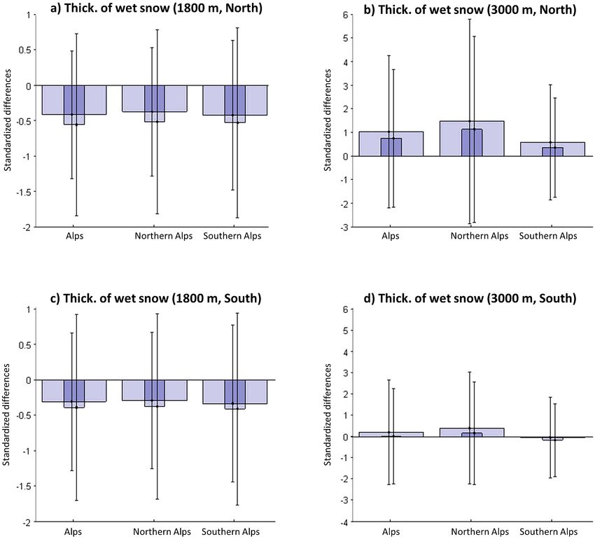
1682 H. Castebrunet et al.: Projected changes of snow conditions and avalanche activity in a warming climate
EM6DATE run when compared to the SCM–ERA40 clima-
tology, and we postulate that these modelling errors are the
same in the climate change runs EM7, 9CS DATE . This conve-
nient assumption has been widely used in previous studies
and is discussed for instance in Wilby et al. (1998) and Deque
(2007). In the present work, we note that the magnitude of the
δmodel correction is small for several variables (Rousselot et
al., 2012).
CS
The meteorological fields EM7CS CENT and EM9CENT were
then used as inputs to drive the detailed snowpack model
Crocus and, subsequently, to compute the MEPRA index for
the two considered 30-year future periods and under the three
different SRES scenarios considered. Simulated SAFRAN
and Crocus data from the daily series on the massif scale
were used to derive anomaly series on the nine larger spatio-
temporal scales corresponding to those studied for the refer-
ence period.
Finally, the nine CI regression models obtained over the
reference period were fed with these projected snow and me-
teorological data (after suitable standardization), using ap-
propriate weighting coefficients (Tables 1–3) and leading to
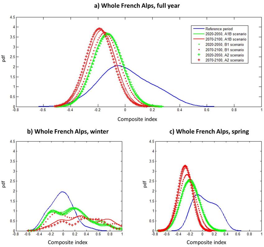
projected values of the avalanche activity index CI for the Figure 3. Probability density functions of the annual and seasonal
two future periods of annual and seasonal avalanche activ- means of the CI regression model over the reference period and in
ity indexes for the nine regions/seasons considered. For ex- 2020–2050 and 2070–2100. The entire French Alps are considered,
ample, Fig. 3 presents the distribution of annual and sea- during the full avalanche year (a) and during the winter (b) and
sonal values of the CI regression model during the refer- spring (c) subperiods.
ence period and the two time periods considered in the fu-
ture on the scale of the entire French Alps. For the refer-
ence period, simulated values are shown as well as a reason- Each climate projection scenario corresponds to 30 years
ably smoothed approximation of their density function from of simulation only, which implies that the significance of
a semi-parametric interpolation of the pseudo-observations changes has to be tested thoroughly as follows:
with a Gaussian kernel smoother. For the future period, for – The significance of differences between future and
clarity, only the smoothed density functions are displayed. reference samples is tested using the Kolmogorov–
Smirnov test.
2.4 Quantitative assessment of changes
– The significance of the difference in mean and variance
Quantitative assessment of changes between the reference is tested using Fisher and Student tests.
period (1961–1990) and the two future periods considered
(2020–2050 and 2070–2100) was made for a selection of According to the statistical theory, we applied Fisher and Stu-
snow and meteorological variables at different elevations and dent tests only for Xt samples for which the normality tested
expositions (Table 5) for the CI (Table 6) and for the MEPRA using the Shapiro–Wilk test was not rejected at the 0.05 sig-
index MI (Table 7). nificance level. Due to the fact that we have only samples of
More precisely, we computed normalized differences in 30 values and that we are considering annual/seasonal means,
means Diffmeans (differences between interannual means – the normality assumption was indeed acceptable most of the
respectively mean(Xt ) and mean(Yt ) where Xt and Yt are time, even for asymmetric variables such as snow depths
the two considered annual (or seasonal) samples) divided by which are generally not Gaussian.
a surrogate of the variability range as Similarly, according to its theoretical setting, the Student
test for means was applied only when the assumption of non-
mean(Yt ) − mean(Xt ) significant differences in variances between the two consid-
Diffmeans = (6) ered Xt and Yt samples could not be rejected. Since variances
max (Xt ) − min(Xt )
between considered samples were often significantly differ-
and variance ratios as ent, this test could be applied less frequently.
We also assessed the probability of future years/seasons
var(Yt ) exceeding the mean and high percentiles of the distribution
Diffvar = . (7) on the reference period. The exceedance probabilities were
var(Xt )
The Cryosphere, 8, 1673–1697, 2014 www.the-cryosphere.net/8/1673/2014/H. Castebrunet et al.: Projected changes of snow conditions and avalanche activity in a warming climate 1683
Table 5. Changes in meteorological and snow variables between the reference period and the two future periods for the entire French Alps
during the whole year and during the winter and the spring periods. “Ref”, 2020–2050 and 2070–2100 correspond, respectively, to the three
considered periods – the reference period (1960–1990) and the mid and end of the 21st century. The probability for a future year to be higher
than the reference mean and the 75 and 95 % percentiles of the reference distribution is quantified, as are ratios and differences between the
reference variance/mean and the two future variances/means. For the Kolmogorov–Smirnov test, bold values indicate different samples at the
0.05 significance level. When the null hypothesis of similar underlying distributions is not rejected, exceedance probabilities appear in italic,
as differences with the reference period may be insignificant. When the assumption of a Gaussian distribution is rejected for at least one of
the considered samples, the significance of the variance comparison cannot be tested so that the variance ratios appear in italic. When the
assumption of Gaussian distributions with similar variances is rejected for at least one of the considered samples, the significance of the mean
comparison cannot be tested so that the mean standardized difference appears in italic. When the significance of variance/mean comparisons
could be tested, ratios/standardized differences rejecting the null hypothesis of equality are shown in bold.
Whole year Distribution comparison Prob. mean Prob. mean Means comparison Variance comparison
(p value, Kolmogorov–Smirnov test) (2020–2050)> (2070–2100)> (standardized differences) (ratios)
Ref/ Ref/ 2020–2050/ Mean q75 q95 Mean q75 q95 2020/2050 2070/2100 2070/2100 2020/2050 2070/2100 2070/2100
2020–2050 2070–2100 2070–2100 (ref) (ref) (ref) (ref) (ref) (ref) ref ref 2020/2050 ref ref 2020/2050
Tmin 1800 m 0.00 0.00 0.00 1 1 0.75 1.00 1.00 1.00 0.76 1.53 0.77 0.99 0.85 0.86
Tmax 1800 m 0.00 0.00 0.00 0.99 0.94 0.54 1.00 1.00 1.00 0.61 1.29 0.68 1.03 0.95 0.92
Tmin 3000 m 0.00 0.00 0.00 1.00 0.99 0.91 1.00 1.00 1.00 0.66 1.33 0.67 0.95 0.95 1.01
Tmax 3000 m 0.00 0.00 0.00 0.99 0.96 0.59 1.00 1.00 1.00 0.57 1.15 0.59 1.01 0.88 0.86
Ptot 1800 m 0.76 0.25 0.65 0.43 0.21 0.01 0.28 0.10 0.00 −0.04 −0.14 −0.09 0.90 0.79 0.87
SP 1800 m 0.00 0.00 0.00 0.07 0.01 0.00 0.00 0.00 0.00 −0.28 −0.51 −0.23 0.66 0.39 0.59
Ptot 3000 m 0.94 0.14 0.41 0.41 0.20 0.01 0.26 0.09 0.00 −0.05 −0.13 −0.08 0.88 0.77 0.87
SP 3000 m 0.03 0.00 0.01 0.21 0.08 0.01 0.03 0.00 0.00 −0.15 −0.33 −0.17 0.77 0.58 0.75
HS (1800 m, north) 0.00 0.00 0.00 0.00 0.00 0.00 0.00 0.00 0.00 −0.52 −0.65 −0.14 0.16 0.05 0.30
HS (3000 m, north) 0.00 0.00 0.00 0.00 0.00 0.00 0.00 0.00 0.00 −0.63 −0.83 −0.21 0.46 0.32 0.68
HS (1800 m, south) 0.00 0.00 0.00 0.00 0.00 0.00 0.00 0.00 0.00 −0.32 −0.38 −0.07 0.08 0.01 0.16
HS (3000 m, south) 0.00 0.00 0.04 0.01 0.00 0.00 0.00 0.00 0.00 −0.39 −0.51 −0.12 0.39 0.25 0.63
HWS (1800 m, north) 0.00 0.00 0.00 0.00 0.00 0.00 0.00 0.00 0.00 −0.41 −0.56 −0.14 0.25 0.11 0.44
HWS (3000 m, north) 0.00 0.00 0.01 1.00 1.00 0.93 0.99 0.99 0.84 1.04 0.76 −0.28 3.39 2.26 0.67
HWS (1800 m, south) 0.00 0.00 0.00 0.01 0.00 0.00 0.00 0.00 0.00 −0.30 −0.39 −0.08 0.16 0.03 0.21
HWS (3000 m, south) 0.01 0.84 0.02 0.77 0.57 0.25 0.54 0.27 0.04 0.21 0.02 −0.19 1.55 0.97 0.62
HDS (1800 m, north) 0.00 0.00 0.00 0.00 0.00 0.00 0.00 0.00 0.00 −0.49 −0.60 −0.11 0.12 0.04 0.36
HDS (3000 m, north) 0.00 0.00 0.00 0.00 0.00 0.00 0.00 0.00 0.00 −0.52 −0.67 −0.14 0.26 0.15 0.57
HDS (1800 m, south) 0.00 0.00 0.00 0.00 0.00 0.00 0.00 0.00 0.00 −0.44 −0.54 −0.10 0.12 0.04 0.37
HDS (3000 m, south) 0.00 0.00 0.03 0.00 0.00 0.00 0.00 0.00 0.00 −0.44 −0.57 −0.13 0.25 0.14 0.58
Tmin 1800 m 0.00 0.00 0.01 0.90 0.69 0.30 0.99 0.93 0.68 0.30 0.53 0.23 0.87 0.87 1.00
Tmax 1800 m 0.00 0.00 0.00 0.84 0.74 0.08 0.98 0.95 0.31 0.20 0.38 0.18 1.00 0.91 0.91
Tmin 3000 m 0.00 0.00 0.01 0.87 0.64 0.26 0.98 0.90 0.61 0.29 0.52 0.23 0.90 0.88 0.98
Tmax 3000 m 0.00 0.00 0.00 0.86 0.69 0.12 0.98 0.94 0.40 0.23 0.44 0.21 0.94 0.82 0.87
Ptot 1800 m 1.00 0.96 1.00 0.47 0.19 0.07 0.46 0.18 0.06 −0.02 −0.03 −0.01 0.93 0.92 0.98
SP 1800 m 0.00 0.00 0.00 0.22 0.03 0.01 0.03 0.00 0.00 −0.17 −0.35 −0.18 0.64 0.44 0.69
Ptot 3000 m 1.00 0.96 1.00 0.48 0.18 0.05 0.47 0.17 0.05 −0.01 −0.02 −0.01 0.93 0.92 0.99
SP 3000 m 1.00 0.96 1.00 0.48 0.18 0.05 0.45 0.16 0.04 −0.02 −0.03 −0.02 0.92 0.88 0.96
HS (1800 m,north) 0.00 0.00 0.00 0.08 0.02 0.00 0.00 0.00 0.00 −0.25 −0.45 −0.20 0.60 0.25 0.42
HS (3000 m, north) 0.03 0.00 0.01 0.19 0.07 0.00 0.04 0.01 0.00 −0.20 −0.37 −0.17 0.75 0.63 0.84
HS (1800 m, south) 0.00 0.00 0.01 0.10 0.01 0.00 0.00 0.00 0.00 −0.18 −0.30 −0.11 0.35 0.07 0.20
HS (3000 m, south) 0.20 0.00 0.26 0.27 0.07 0.00 0.11 0.01 0.00 −0.15 −0.26 −0.11 0.85 0.67 0.79
HWS (1800 m, north) 0.01 0.00 0.84 0.66 0.54 0.19 0.76 0.66 0.16 0.27 0.33 0.06 2.39 2.81 1.17
HWS (3000 m, north) 0.03 0.00 0.00 0.44 0.72 0.39 0.76 0.84 0.72 0.17 1.26 1.10 7.74 102.90 13.30
HWS (1800 m, south) 0.76 0.08 0.02 0.39 0.16 0.07 0.19 0.06 0.00 −0.02 −0.17 −0.15 1.25 0.36 0.29
HWS (3000 m, south) 0.11 0.00 0.15 0.54 0.30 0.13 0.68 0.37 0.10 0.13 0.20 0.07 2.01 2.35 1.17
HDS (1800 m, north) 0.00 0.00 0.00 0.07 0.00 0.00 0.00 0.00 0.00 −0.27 −0.44 −0.17 0.44 0.15 0.35
HDS (3000 m, north) 0.20 0.00 0.08 0.29 0.06 0.01 0.10 0.01 0.00 −0.12 −0.23 −0.11 0.66 0.43 0.65
HDS (1800 m, south) 0.00 0.00 0.00 0.08 0.00 0.00 0.00 0.00 0.00 −0.24 −0.38 −0.15 0.38 0.14 0.38
HDS (3000 m, south) 0.20 0.04 0.26 0.32 0.07 0.01 0.16 0.01 0.00 −0.11 −0.20 −0.08 0.70 0.47 0.68
Tmin 1800 m 0.00 0.00 0.00 0.99 0.96 0.66 1.00 1.00 0.98 0.50 0.86 0.36 0.84 0.92 1.10
Tmax 1800 m 0.00 0.00 0.00 0.97 0.83 0.60 1.00 1.00 0.98 0.45 0.92 0.47 0.86 1.04 1.21
Tmin 3000 m 0.00 0.00 0.00 0.97 0.89 0.58 1.00 0.99 0.94 0.36 0.64 0.29 0.84 0.99 1.17
Tmax 3000 m 0.00 0.00 0.00 0.96 0.89 0.46 1.00 1.00 0.93 0.36 0.73 0.36 0.85 1.00 1.19
Ptot 1800 m 1.00 0.88 0.48 0.54 0.27 0.08 0.45 0.19 0.05 0.02 −0.03 −0.05 1.06 1.01 0.96
SP 1800 m 0.00 0.00 0.01 0.06 0.00 0.00 0.00 0.00 0.00 −0.31 −0.47 −0.17 0.51 0.26 0.52
Ptot 3000 m 0.94 0.29 0.46 0.53 0.33 0.04 0.43 0.25 0.02 0.02 −0.03 −0.05 1.04 0.98 0.95
SP 3000 m 0.34 0.00 0.01 0.40 0.22 0.02 0.12 0.04 0.00 −0.05 −0.21 −0.16 0.97 0.70 0.72
HS (1800 m, north) 0.00 0.00 0.00 0.00 0.00 0.00 0.00 0.00 0.00 −0.39 −0.56 −0.18 0.31 0.07 0.23
HS (3000 m, north) 0.01 0.00 0.03 0.18 0.04 0.00 0.03 0.00 0.00 −0.25 −0.54 −0.28 0.96 1.00 1.04
HS (1800 m, south) 0.00 0.00 0.00 0.01 0.00 0.00 0.00 0.00 0.00 −0.24 −0.30 −0.06 0.09 0.01 0.09
HS (3000 m, south) 0.01 0.00 0.07 0.21 0.05 0.01 0.04 0.00 0.00 −0.20 −0.37 −0.17 0.92 0.67 0.72
HWS (1800 m, north) 0.00 0.00 0.00 0.03 0.00 0.00 0.00 0.00 0.00 −0.34 −0.57 −0.23 0.43 0.11 0.25
HWS (3000 m, north) 0.00 0.00 0.27 0.97 0.97 0.74 0.99 0.99 0.87 0.66 0.86 0.21 2.57 3.20 1.25
HWS (1800 m, south) 0.00 0.00 0.00 0.06 0.00 0.00 0.00 0.00 0.00 −0.25 −0.32 −0.08 0.15 0.01 0.07
HWS (3000 m, south) 0.00 0.09 0.17 0.81 0.65 0.22 0.71 0.54 0.17 0.26 0.18 −0.08 1.50 1.76 1.17
HDS (1800 m, north) 0.00 0.00 0.01 0.01 0.00 0.00 0.00 0.00 0.00 −0.33 −0.44 −0.11 0.27 0.11 0.40
HDS (3000 m, north) 0.05 0.00 0.03 0.15 0.05 0.00 0.01 0.00 0.00 −0.20 −0.35 −0.15 0.54 0.33 0.62
HDS (1800 m, south) 0.00 0.00 0.04 0.01 0.00 0.00 0.00 0.00 0.00 −0.34 −0.46 −0.12 0.27 0.10 0.37
HDS (3000 m, south) 0.03 0.00 0.01 0.16 0.03 0.00 0.01 0.00 0.00 −0.20 −0.36 −0.17 0.51 0.29 0.57
T : temperature; Ptot : total precipitation; SP: snow precipitation; HS: snow depth; HWS : thickness of wet snow; HDS : thickness of recent surface dry snow.
www.the-cryosphere.net/8/1673/2014/ The Cryosphere, 8, 1673–1697, 20141684 H. Castebrunet et al.: Projected changes of snow conditions and avalanche activity in a warming climate
Table 6. Changes in CI models between the reference period and the two future periods. “Ref”, 2020–2050 and 2070–2100 correspond,
respectively, to the three considered periods – the reference period (1960–1990) and the middle and end of the 21st century. Details of the
table are the same as for Table 5.
Distribution comparison Prob. mean Prob. mean Means comparison Variance comparison
(p value, Kolmogorov–Smirnov test) (2020–2050)> (2070–2100)> (standardized differences) (ratios)
Ref/ Ref/ 2020–2050/ Mean q75 q95 Mean q75 q95 2020/2050 2070/2100 2070/2100 2020/2050 2070/2100 2070/2100
2020–2050 2070–2100 2070–2100 (ref) (ref) (ref) (ref) (ref) (ref) – ref – ref – 2020/2050 – ref – ref – 2020/2050
French Alps, year 0.00 0.00 0.00 0.00 0.00 0.00 0.04 0.00 0.00 -0.19 -0.26 -0.06 0.06 0.03 0.44
French Alps, winter 0.01 0.00 0.01 0.72 0.61 0.44 0.87 0.80 0.70 0.30 1.27 0.97 4.34 37.43 8.62
French Alps, spring 0.00 0.00 0.01 0.01 0.00 0.00 0.00 0.00 0.00 −0.43 −0.56 −0.13 0.41 0.20 0.48
North. French Alps, year 0.00 0.00 0.07 0.00 0.00 0.00 0.00 0.00 0.00 −0.44 −0.54 −0.10 0.31 0.24 0.78
North. French Alps, winter 0.20 0.00 0.22 0.32 0.10 0.00 0.12 0.01 0.00 −0.10 −0.21 −0.10 0.62 0.39 0.63
North. French Alps, spring 0.00 0.00 0.00 0.01 0.00 0.00 0.00 0.00 0.00 −0.42 −0.63 −0.22 0.45 0.22 0.49
South. French Alps, year 0.00 0.00 0.36 0.02 0.00 0.00 0.00 0.00 0.00 −0.30 −0.33 −0.03 0.11 0.03 0.29
South. French Alps, winter 0.05 0.00 0.03 0.62 0.50 0.29 0.87 0.80 0.56 0.31 0.95 0.64 7.05 24.32 3.45
South. French Alps, spring 0.00 0.00 0.00 0.05 0.02 0.00 0.01 0.00 0.00 −0.29 −0.36 −0.07 0.19 0.09 0.46
Table 7. Changes in MEPRA index between the reference period and the two future periods. “Ref”, 2020–2050 and 2070–2100 correspond,
respectively, to the three considered periods – the reference period (1960–1990) and the middle and end of the 21st century, respectively.
Details of the table are the same as for Table 5.
Distribution comparison Prob. mean Prob. mean Means comparison Variance comparison
(p value, Kolmogorov–Smirnov test) (2020–2050)> (2070–2100)> (standardized differences) (ratios)
Ref/ Ref/ 2020–2050/ Mean q75 q95 Mean q75 q95 2020/2050 2070/2100 2070/2100 2020/2050 2070/2100 2070/2100
2020–2050 2070–2100 2070–2100 (ref) (ref) (ref) (ref) (ref) (ref) – ref – ref – 2020/2050 – ref – ref – 2020/2050
French Alps, year 0.34 0.00 0.00 0.37 0.17 0.01 0.05 0.01 0.00 −0.08 −0.31 −0.23 0.93 0.53 0.58
French Alps, winter 0.20 0.00 0.17 0.33 0.16 0.00 0.13 0.03 0.00 −0.08 −0.18 −0.09 0.77 0.49 0.65
French Alps, spring 0.34 0.01 0.00 0.59 0.34 0.08 0.20 0.05 0.00 0.08 −0.23 −0.31 1.21 0.75 0.62
North. French Alps, year 0.54 0.00 0.00 0.44 0.26 0.02 0.09 0.02 0.00 −0.04 −0.26 −0.22 1.01 0.59 0.58
North. French Alps, winter 0.54 0.02 0.18 0.39 0.20 0.00 0.16 0.05 0.00 −0.06 −0.16 −0.10 0.83 0.52 0.62
North. French Alps, spring 0.20 0.13 0.03 0.65 0.39 0.14 0.29 0.08 0.01 0.12 −0.14 −0.26 1.39 0.91 0.66
South. French Alps, year 0.00 0.00 0.00 0.32 0.20 0.08 0.19 0.10 0.03 −0.16 −0.31 −0.15 0.87 0.55 0.63
South. French Alps, winter 0.03 0.00 0.37 0.27 0.15 0.02 0.21 0.10 0.01 −0.17 −0.23 −0.06 0.65 0.49 0.76
South. French Alps, spring 0.54 0.00 0.00 0.38 0.24 0.08 0.18 0.10 0.01 −0.05 −0.25 −0.20 1.17 0.68 0.58
computed from the normal fit on the Xt samples when possi- the previous study (e.g. snow conditions on slopes and re-
ble (i.e. when the Gaussian assumption could not be rejected) cent surface dry/wet snow thickness). Figures 4–8 illustrate
and from the Kernel smoothing approximation of the empir- regional north–south differences with regard to the whole
ical cumulative distribution function (cdf), introduced previ- French Alps, while Table 5 shows detailed results for the en-
ously, otherwise. tire French Alps only but only displays results for the three
Finally, we also tested the difference between the multi- considered time periods, highlighting seasonal variations. In
variate distributions of annual/seasonal variables correspond- what follows we focus on projections concerning the A1B
ing to each of the CI models (that is, for each of the nine re- scenario (IPCC, 2007) only.
gression models, the joint distribution of the variables Xjnorm
t , In Table 5, it is important to note that differences in prob-
j = [1, P ] number of covariates), using the Cramer test (Ta- abilities of exceeding percentiles can be insignificant if un-
ble 8). derlying distributions are not different (null hypothesis not
rejected by the Kolmogorov–Smirnov test). Hence, signif-
icant differences are shown in bold; for the whole year, it
3 Results is generally the case for all variables between reference and
2020–2050 periods, except for the total precipitation and for
3.1 Meteorological and snowpack conditions in the
the thickness of wet snow at 3000 m for a south-facing slope.
future
Similarly, normalized differences in interannual means and
Meteorological and snowpack conditions in the future on variance ratios are often high and far from 1, respectively,
the massif and annual scales are presented and discussed but testing the significance of these changes could not always
in detail by Rousselot et al. (2012). Here, we complement be done, depending on the Shapiro–Wilk and Fisher test re-
the analysis by assessing changes between reference and fu- sults. Significant differences are shown in bold whereas val-
ture periods in terms of probabilities of exceeding distribu- ues whose significance could not be tested are shown in grey.
tion percentiles during the reference period in the future and
by assessing normalized differences and ratios for the nine 3.1.1 Temperatures
spatio-temporal scales we consider. We also expand this ap-
proach to snowpack variables that are more directly rele- As expected, between the reference period and the mid 21st
vant for avalanche activity and that were not considered in century, temperatures were found to increase significantly.
The Cryosphere, 8, 1673–1697, 2014 www.the-cryosphere.net/8/1673/2014/You can also read