Use of Sentinel-1 radar observations to evaluate snowmelt dynamics in alpine regions
←
→
Page content transcription
If your browser does not render page correctly, please read the page content below
The Cryosphere, 14, 935–956, 2020
https://doi.org/10.5194/tc-14-935-2020
© Author(s) 2020. This work is distributed under
the Creative Commons Attribution 4.0 License.

Use of Sentinel-1 radar observations to evaluate
snowmelt dynamics in alpine regions
Carlo Marin1 , Giacomo Bertoldi2 , Valentina Premier1 , Mattia Callegari1 , Christian Brida2 , Kerstin Hürkamp3 ,
Jochen Tschiersch3 , Marc Zebisch1 , and Claudia Notarnicola1
1 Institute
          for Earth Observation, Eurac Research, Viale Druso, 1 39100 Bolzano, Italy
2 Institute
          for Alpine Environment, Eurac Research, Viale Druso, 1 39100 Bolzano, Italy
3 Helmholtz Zentrum München, German Research Center for Environmental Health, Institute of Radiation Medicine,

Ingolstädter Landstraße 1, 85764 Neuherberg, Germany

Correspondence: Carlo Marin (carlo.marin@eurac.edu)

Received: 25 July 2019 – Discussion started: 4 September 2019
Revised: 22 January 2020 – Accepted: 7 February 2020 – Published: 12 March 2020

Abstract. Knowing the timing and the evolution of the snow          directly correlated to the SWE decrease but to the different
melting process is very important, since it allows the pre-         snow conditions, which change the backscattering mecha-
diction of (i) the snowmelt onset, (ii) the snow gliding and        nisms. Finally, we show a spatially distributed application
wet-snow avalanches, (iii) the release of snow contaminants,        of the identification of the runoff onset from SAR images
and (iv) the runoff onset. The snowmelt can be monitored            for a mountain catchment, i.e., the Zugspitze catchment in
by jointly measuring snowpack parameters such as the snow           Germany. Results allow us to better understand the spatial
water equivalent (SWE) or the amount of free liquid wa-             and temporal evolution of melting dynamics in mountain re-
ter content (LWC). However, continuous measurements of              gions. The presented investigation could have relevant appli-
SWE and LWC are rare and difficult to obtain. On the other          cations for monitoring and predicting the snowmelt progress
hand, active microwave sensors such as the synthetic aper-          over large regions.
ture radar (SAR) mounted on board satellites are highly sen-
sitive to LWC of the snowpack and can provide spatially dis-
tributed information with a high resolution. Moreover, with
the introduction of Sentinel-1, SAR images are regularly ac-        1   Introduction
quired every 6 d over several places in the world. In this paper
we analyze the correlation between the multitemporal SAR            Seasonal snowpack is one of the most important water re-
backscattering and the snowmelt dynamics. We compared               sources present in nature. It stores water during the winter
Sentinel-1 backscattering with snow properties derived from         and releases it in spring during the melt. In mountain regions,
in situ observations and process-based snow modeling simu-          snow storage is essential for the freshwater supply of the low-
lations for five alpine test sites in Italy, Germany and Switzer-   lands, making the mountains the water towers of the down-
land considering 2 hydrological years. We found that the            stream regions (Viviroli and Weingartner, 2004). In fact, the
multitemporal SAR measurements allow the identification of          temporally delayed release of the water from the head water-
the three melting phases that characterize the melting pro-         sheds to the forelands is essential for a large number of hu-
cess, i.e., moistening, ripening and runoff. In particular, we      man activities such as agriculture irrigation, drinking water
found that the C-band SAR backscattering decreases as soon          supply and hydropower production (Beniston et al., 2018). In
as the snow starts containing water and that the backscatter-       particular, in the Alps, discharges in May and June are largely
ing increases as soon as SWE starts decreasing, which cor-          dictated by snowmelt, while from July to September they are
responds to the release of meltwater from the snowpack. We          influenced by glacier melt (Wehren et al., 2010) and liquid
discuss the possible reasons of this increase, which are not        precipitation. On the other hand, wet snow may contribute to
                                                                    natural disasters such as wet-snow avalanches (Bellaire et al.,

Published by Copernicus Publications on behalf of the European Geosciences Union.
936                                       C. Marin et al.: Use of Sentinel-1 to evaluate snowmelt dynamics in alpine regions

2017) or wet-snow gliding (Fromm et al., 2018). Moreover,            ing of LWC. In particular, three systems have demonstrated
in case of accumulated contaminant release from a snow-              to be effective and robust in operational conditions: (i) the
pack, initial runoff meltwater can be highly enriched and is         snowpack analyzer (SPA) (Stähli et al., 2004), (ii) the snow
able to cause severe impact on the water quality (Hürkamp            sense (Koch et al., 2014) based on GPS signals, and (iii) the
et al., 2017). In this context, knowing the temporal and spa-        upward-looking ground-penetrating radar (upGPR) (Schmid
tial evolution of the snow melting process is very important         et al., 2014). All of them are commercial systems buried un-
for a proactive management of the water resources and for            der the snowpack and rely on different methods for the di-
hazard mitigation.                                                   electric constant estimation. Interestingly, these EM devices
   The melt period can be generally separated in three phases        can be used to measure the SWE as well. However, all these
(Dingman, 2015): (i) moistening, (ii) ripening and (iii)             ground-based measurements are limited in application to a
runoff. The moistening is the initial phase of the snowmelt.         single point; require calibration to relate the dielectric con-
The air temperature and solar radiation increase, and due to         stant to volumetric snow LWC; and some of them are expen-
heat exchanges and/or rain the superficial layers of the snow-       sive, power intensive and laborious to install and maintain.
pack start melting. The ripening phase begins when the maxi-         These limitations complicate the possibility to monitor and
mum retention capacity of the pores is exceeded. The wetting         understand the meltwater runoff and the snow stability con-
front penetrates through the snowpack, driven by repeated            sidering also the spatial variability of the snowmelt dynam-
cycles of melting and refreezing, but the meltwater is not yet       ics.
released. During this phase, the snowpack becomes isother-              To mitigate these limitations, energy-based, multilayer
mal, and when no more liquid water can be retained, the              physically based snow models can simulate SWE and LWC
runoff phase starts. The snowmelt process is a nonlinear pro-        at high spatial and temporal resolution (Essery et al., 2013).
cess affected by the strong variability of both the snowpack         Such kinds of models account for shading, shortwave and
characteristics and the meteorological forcings that affect the      longwave radiation, and turbulent fluxes of sensible and
snow. In order to obtain useful information about the pro-           latent heat (Mott et al., 2011) but can differ in the way
gression of the melting process, noninvasive techniques that         they parametrize snow metamorphism, grain size evolu-
allow performing multiple measurements at the same loca-             tion, snow layering and liquid water percolation (Wever
tion should be exploited. For this purpose, measurements of          et al., 2014). They can range from very detailed approaches
meteorological variables such as air temperature, snow tem-          with a Lagrangian representation of snow layers such as
perature, relative humidity, wind speed, precipitation and so-       avalanche-forecasting models like CROCUS (Brun et al.,
lar radiation are usually employed to extract information on         1992) or SNOWPACK/ALPINE3D (Bartelt and Lehning,
snowmelt dynamics (Kinar and Pomeroy, 2015). However,                2002; Lehning et al., 2006) to more simplified approaches
the most significant state variables to properly identify the        such as the ones of hydrologically oriented Eulerian mod-
three melting phases are the snow water equivalent (SWE),            els like AMUNDSEN (Strasser et al., 2011) or GEOtop (En-
i.e. the total mass of liquid and solid water stored in the form     drizzi et al., 2014). Therefore, snow models can provide de-
of snow; and the liquid water content (LWC), i.e. the mass           tailed information about the snow properties starting from
of liquid water inside the snowpack. An increase in LWC              observed meteorological conditions, which can be reliably
in time indicates that a moistening process is ongoing. The          acquired especially at the plot scale. However, model per-
downward penetration of the water front into the snowpack            formances are affected by uncertainties and errors related to
leads first to a partial and later to a complete isothermal state.   model structure (Avanzi et al., 2016), meteorological forc-
This leads to the generation of water runoff and consequently        ing (Raleigh et al., 2015) and model parametrizations (En-
to a significant decrease in SWE.                                    gel et al., 2017; Günther et al., 2019). Therefore, there is the
   Continuous measurements of SWE and LWC are therefore              need of snow observations with high temporal and spatial
essential to monitor the snowpack melting dynamics. So far,          resolution, distributed over a large area and systematically
the most common method to manually measure SWE is us-                acquired.
ing snow sampling tubes, while the most spread techniques               In the past years, synthetic aperture radar (SAR) was
for automatic SWE measurement include snow pillows and               shown to be a valid tool to identify the wet snow, i.e., snow
snow scales (Kinar and Pomeroy, 2015). The installation and          that contains a given amount of free liquid water (Nagler
the maintenance of these kinds of measurements are very              and Rott, 2000; Dong, 2018). In fact, SAR measurements
costly and a relatively limited number of continuous mea-            are highly sensitive to the liquid water in the snowpack, and
surements of SWE are available in the Alps. Direct measure-          the increase in the LWC causes a high dielectric loss that
ments of LWC are usually performed through empirical es-             increases the absorption coefficient generating backscattered
timations (e.g., the hand test) or indirect assessments based        signal with low intensity (Long and Ulaby, 2015). This phys-
on snow temperature. Recently, some promising systems that           ical principle has been exploited for the generation of wet-
exploit the dielectric properties of the snow in the microwave       snow maps by the bitemporal algorithm proposed by Nagler
region of the electromagnetic (EM) spectrum have been pre-           and Rott (2000) and further improved in Nagler et al. (2016).
sented to allow the continuous and nondestructive measur-            However, the increase in the liquid water content explains

The Cryosphere, 14, 935–956, 2020                                                         www.the-cryosphere.net/14/935/2020/
C. Marin et al.: Use of Sentinel-1 to evaluate snowmelt dynamics in alpine regions                                            937

only partially the decrease in the backscattering coefficient.     distributed information about the melting phases of the snow-
Indeed, as pointed out in Shi and Dozier (1995) and Bagh-          pack in alpine terrain, which can be used for monitoring and
dadi et al. (2000), the relationship between the coefficient       predicting the snowmelt progress over large regions.
of backscattering and the snow wetness can cause an incre-
ment of the backscattering value depending on the conditions
of the snow roughness, snow density, snow layering, snow           2     Background
grain size and local incidence angle. This large number of
unknowns, upon which the SAR backscattering is dependent,          In this section we report the theoretical background on which
defines a complex multiparametric problem that is difficult        this work is based. First, the snow melting process is ex-
or even impossible to solve without introducing some sim-          plained from a physical point of view, and the different
plification assumptions. So, even though some works have           phases are identified considering the information of LWC
been presented that try to extract the LWC using C-band            and SWE. Then, the response of the SAR backscattering to
SAR images (Shi and Dozier, 1995; Longepe et al., 2009),           the wet snow is described in detail.
to the best of our knowledge there are no attempts to use the
SAR as source of information for describing the multitem-          2.1    Snow melting process
poral evolution of the snow melting process. Progress has
been hampered by (i) the lack of ground truth information,         Figure 1 illustrates the snow cover development during the
(ii) the relatively high number of sources of uncertainty of       melting season considering the snow status in the morning
the SAR signal, and (iii) the difficulty in accessing SAR data     and in the afternoon, when the S-1 descending and ascending
in the past. This has changed since 2014 with the introduc-        data are acquired respectively. Hypothetical values of LWC
tion of the Sentinel-1 (S-1) mission from the European Space       and SWE are reported on the right side of the figure. In gen-
Agency (ESA) and the European Commission (EC) guaran-              eral, the liquid water is introduced in the snow by rain and/or
teeing the availability of C-band SAR images free of charge.       melt due to heat exchange and the incoming flux of short-
Specifically, S-1 is a constellation made up of two near-polar     wave radiation flux, which varies with slope, aspect and ele-
sun-synchronous satellites that acquire images early in the        vation. In both cases, the snowpack starts melting at the sur-
morning and late in the afternoon, with a revisit time of 6 d      face (Techel and Pielmeier, 2011). This superficial moisten-
at the Equator. Moreover, as discussed before, an increas-         ing phase can be identified by comparing observations from
ing number of data on relevant snow parameters related to          the coldest and warmest period of the day; i.e., a diurnal cy-
the snowmelt are collected by operational systems (e.g., by        cle is visible. Interestingly, the SAR acquisitions are approx-
SPA) or derived by physically based snow models. The infor-        imately acquired around these two periods. The liquid wa-
mation on SWE and LWC provided by independent sources              ter released or absorbed from the superficial layers gets in
opens new opportunities for better understanding the rela-         contact with the subfreezing snow present underneath and
tionship between the snowpack properties during the melting        freezes. This releases latent heat that causes the snowpack to
phase and the multitemporal SAR backscattering.                    warm up, starting the process of snow ripening. Repeated cy-
   The aim of this work is to evaluate the information that        cles of partial melting during the day and refreezing during
S-1 can provide on monitoring the snowmelt dynamics. In            the night induce the development of the wetting front into
particular, we provide the theoretical EM background for un-       the snow. This is generally not uniform, since infiltrations
derstanding the impact on the multitemporal SAR backscat-          usually start through isolated “flow fingers” which enlarge
tering of a melting snowpack. Then, we analyze the relation-       into meltwater channels due to the passing of time. There-
ship between the multitemporal SAR signal acquired from            fore, the ripening of the snowpack may be different year by
S-1 and in situ measurements of LWC and SWE in the Alps.           year or considering different areas. In fact, climatic factors
Given the limited number of point-related continuous SWE           or snowpack stratifications may induce different behaviors.
and LWC measurements available in the test area, we made           At the point of full water saturation, the snow layer cannot
use of the physically based model SNOWPACK to simulate             retain any more liquid water. Further absorption of energy
the snow properties in other locations where only meteoro-         produces water output, which, depending on soil properties,
logical data and snow depth were available. This allowed           ice and water content, could infiltrate the soil or appear as
us to define five test sites at different altitudes in the Alps,   surface runoff (DeWalle and Rango, 2008). The runoff phase
where the interactions of S-1 backscattering with the snow-        is characterized by a significant decrease in SWE.
pack were studied in detail during two melting seasons. On            During the melting, the presence of liquid water inside
the basis of the outcomes of the study, we propose an inter-       the snowpack directly affects the grain size, the grain shape
pretation scheme to be applied to multitemporal dual polar-        and the density of the pack (Pomeroy and Brun, 2001). In-
ization C-band SAR data in order to identify the different         deed, during the melt process the snow undergoes to a rapid
snow melting phases of moistening, ripening and runoff. Fi-        metamorphism that leads to a growing and a rounding of the
nally, we demonstrate the effectiveness of the proposed ap-        grains linked to an increase in the snow density. Moreover, it
proach in a real application scenario to provide a spatially       is important to underline that during the melt season a gen-

www.the-cryosphere.net/14/935/2020/                                                        The Cryosphere, 14, 935–956, 2020
938                                          C. Marin et al.: Use of Sentinel-1 to evaluate snowmelt dynamics in alpine regions

                                                                          these contributions depends on parameters related to (i) the
                                                                          sensors, i.e., frequency, local incidence angle (LIA) and po-
                                                                          larization; (ii) the snowpack properties, i.e., liquid water con-
                                                                          tent, density (DS), ice particle size and shape (GS), and sur-
                                                                          face roughness (RS), which is usually described by the stan-
                                                                          dard deviation of the height and the correlation length of
                                                                          the surface; and (iii) the ground properties. In this paper we
                                                                          focus on the use of the C-band SAR mounted on board S-
                                                                          1, and therefore all the parameters related to the sensor are
                                                                          known. Nonetheless, deriving the theoretical behavior of the
                                                                          time series of σ 0 for a given LIA for 1 hydrological year
                                                                          is complex. Indeed, the relationship between the backscat-
                                                                          tering and the snow parameters forms a nonlinear system of
                                                                          equations. In the following we identify the main scattering
                                                                          mechanisms isolating the contribution of each parameter to
                                                                          the total backscattering.
                                                                             During the accumulation period, dry snow is almost trans-
                                                                          parent for the C band, and the radar echo can penetrate the
                                                                          snow for several meters. In this situation, the main scatter-
                                                                          ing source is the snow–ground interface (see Fig. 2), and the
                                                                          backscattering is almost insensitive to different snow param-
Figure 1. Example of transitions in snow status during the melting
season obtained by sampling the snow in the morning (M), when the
                                                                          eters (Rott and Mätzler, 1987; Shi and Dozier, 1993). During
S-1 descending observations are taken, and in the evening (A), when       the melting period, the increase in the free liquid water inside
the S-1 ascending data are taken. The upper part of the figure illus-     the snowpack causes high dielectric losses, which increase
trates the simplified temporal transportation of the free liquid water    the absorption coefficient. By considering a sufficiently thick
                                                                          snowpack, this leads to a rapid decrease in σgrd   0 , which can
(blue area) in the dry snowpack (white area). The lower part of the
figure illustrates the respective temporal evolution of LWC (yellow       then be neglected. By assuming all the parameters but the
line) and SWE (red line). Specifically, by starting from a dry situ-      LWC to be constant, the increase in LWC causes the volume
ation, the liquid water is introduced into the snowpack by either a       scattering to decrease and the backscattering becomes sensi-
rain event or the melt due to the incoming flux of shortwave radi-        tive to surface roughness (Shi and Dozier, 1995). When the
ation. In this moistening phase the LWC (yellow line) varies with         surface is smooth, for example, according to the Fraunhofer
a diurnal cycle. Repeated cycles of partial melting and refreezing
                                                                          criterion (Long and Ulaby, 2015), volume scattering domi-
conduct the snowpack to the isothermal state. During the ripening
period, a combination of different situations can occur depending
                                                                          nates and therefore the increase in LWC results in a decrease
on the weather conditions, but an increasing trend of the LWC is          in the total backscattering, whereas when the surface is rough
visible. Once the snowpack is isothermal and it cannot retain water       the surface scattering dominates; thus with the increase in
anymore, it starts to produce water output until it melts totally. This   LWC the total backscattering tends to increase. The amount
last phase starts with a significant decrease in the SWE (red line).      of wetness from which the surface scattering becomes pre-
                                                                          dominant depends mainly on the surface roughness and LIA
                                                                          and may vary from about 1 % to 6 % of the total volume (Ma-
eral increase in the roughness of the snow surface is observed            gagi and Bernier, 2003). However, other parameters play a
(Fassnacht et al., 2009) due to localized melting pattern (i.e.,          role in this mechanism: by assuming all the parameters but
flow fingers) and rain-on-snow events.                                    the snow density to be constant, the volume scattering de-
                                                                          creases as the snow density increases, if all the other param-
2.2   SAR backscattering response to wet snow                             eters are kept fixed. In contrast, the grain size increases the
                                                                          volume scattering. Finally, it is worth stressing the fact that
From an EM point of view, the snowpack is an inhomoge-
                                                                          the response to the wet snow becomes more complex in case
neous medium composed of scattering elements with differ-
                                                                          of the snowpack in forest (Koskinen et al., 2010). In this case
ent sizes, shapes, orientations and permittivity values. The
                                                                          the total backscattering σ 0 is also a function of the forest
backscattering σ 0 produced by an EM wave generated by
                                                                          stem volume. This can be estimated and taken into account;
SAR over such a medium can be modeled as an incoherent
                                                                          nonetheless in this work we focus on the identification of the
sum of three contributions (Shi and Dozier, 1995; Long and
                                                                          snow melting phase in open areas.
Ulaby, 2015): the surface scattering produced at the air–snow
            0 ; the surface scattering produced at the snow–                 The main scattering mechanisms and their influence on
interface, σsup
                                                                          the backscattering, as studied in the literature, are reported
ground interface attenuated by the snowpack, σgrd 0 ; and the
                                                                          in Table 1. Even though the table reports the main backscat-
                                          0
volumetric scattering of the snowpack, σvol . The intensity of            tering mechanisms of the different snow conditions during

The Cryosphere, 14, 935–956, 2020                                                               www.the-cryosphere.net/14/935/2020/
C. Marin et al.: Use of Sentinel-1 to evaluate snowmelt dynamics in alpine regions 939
Figure 2. Main SAR backscattering mechanisms in presence of dry and wet snow at the C band. The dry snow is almost transparent, and
the radar echo can penetrate the snow for several meters. The presence of LWC causes high dielectric loss, which increases the absorption
coefficient.
Table 1. Simplified SAR backscattering response to wet snow di- 3 Dataset description
0 , and surface backscattering, σ 0 , contri-
vided in volumetric, σvol sup
butions. Considering a sufficiently thick snowpack the contribution In this section, we present the experimental sites, and we de-
0 can be neglected.
of σgrd scribe the collected in situ data, the SNOWPACK setup and
S-1 data.
Parameter 0
σvol 0
σsup
Liquid water content (LWC) negative correlation positive correlation 3.1 Test site description and in situ data
Snow density (DS) negative correlation positive correlation
Snow grain size (GS) positive correlation – For ground truth and as input for the simulations with
Surface roughness (RS) – positive correlation
SNOWPACK, we consider five snow and meteorological
weather stations with a different location in terms of place
and altitude in the European Alps, equipped with different in-
the melting process, the complete multitemporal behavior stalled sensors. Among these, one is located in Bavaria (Ger-
that characterizes the three phases of moistening, ripening many), three in South Tyrol (Italy) and one in Graubünden
and runoff has not yet been studied. In particular, from an (also known as Grisons, Switzerland). Specifically, the con-
EM modeling point of view or real-data analysis, the im- sidered parameters are wind velocity (VW), wind direction
plications of the wet-snow metamorphism – i.e., increase (DW), air temperature (TA), relative humidity (RH), snow
in LWC, density, snow grain size and superficial roughness depth (HS), snow temperature at different depths (TS), sur-
– remain mainly unsolved. Indeed, state-of-the-art radiative face temperature (TSS), soil temperature (TSG), incoming
transfer (RT) models, particularly designed for studying the shortwave radiation (ISWR), incoming longwave radiation
snow melting process, such as Shi and Dozier (1995), Nagler (ILWR), outgoing shortwave radiation (OSWR), snow wa-
and Rott (2000), and Magagi and Bernier (2003), are not able ter equivalent (SWE), snow density (DS), liquid water con-
to model the microstructure scattering interactions, whereas tent (LWC) and ice content (IC). The considered data records
RT models that take into account the microstructure interac- started from 1 October 2016 in order to cover the two winter
tions, such as the models developed in SMRT (Picard et al., seasons 2016/2017 and 2017/2018. An overview of the loca-
2018) or MEMLS3&a (Proksch et al., 2015), are not able tion of the stations is presented in Fig. 3, and a summary with
to model the contribution from the superficial roughness and the available parameters is presented in Table 2.
have never been specifically tested for the characterization of
the melting phases. Therefore, without further research and 3.1.1 Zugspitze (Werdenfelser Alps, Germany)
validation activities, this invalidates the possibility of using
state-of-the-art RT models to better understand the multitem- The station is located in the northern Calcareous Werden-
poral EM mechanisms during the snowmelt at the C band felser Alps, being part of the Zugspitze massif. It is part
(e.g., Veyssière et al., 2018, found a significant deviation be- of the snow monitoring stations network of the Bavarian
tween observations and simulations with MEMLS3&a dur- Avalanche Warning Service (Lawinenwarnzentrale Bayern)
ing the melting period). and located on a flat plateau at the southern slope of the
In the following, as first attempt to fill this gap, we will Zugspitze summit (2962 m a.s.l.), the so-called Zugspitzplatt
consider the real time series of backscattering recorded by (1500–2700 m a.s.l.), which is surrounded by several sum-
S-1 during 2 hydrological years in the proximity of five test mits in the north, south and west and drained by the Part-
sites where LWC and SWE were measured or simulated. The nach river to the east. In addition to being a standard me-
outcome of this study will be exploited to (i) understand if a teorological station, the site is equipped with a snow scale
characteristic relation can be recognized from the compari- and a snow pack analyzer to record SWE, DS, LWC and IC.
son between the multitemporal SAR signal and the melting The SPA uses a time-domain reflectometer (TDR) at high
phases and (ii) define some rules to automatically identify the frequencies and a low-frequency impedance analyzer. By ex-
beginning of each melting phase from the time series of σ 0 . ploiting different frequencies, the SPA is able to determine
www.the-cryosphere.net/14/935/2020/ The Cryosphere, 14, 935–956, 2020940 C. Marin et al.: Use of Sentinel-1 to evaluate snowmelt dynamics in alpine regions
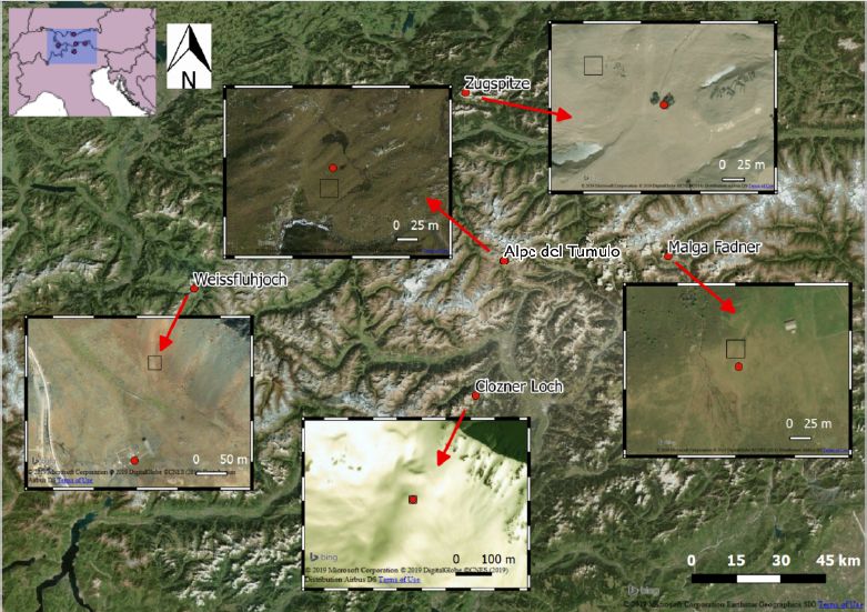
Figure 3. Overview map with the five stations used for the presented study (© 2019 Microsoft Corporation, © 2019 Digital Globe, © CNES
(2019) Distribution Airbus DS). The red points indicate the exact location of the stations. The black squares indicate the S-1 footprints. The
footprints were selected in order to minimize any possible interference of the EM wave with the homemade structures but maintaining a
certain correlation with the in situ measurements. The panoramic images give an idea about the land cover type and the topography around
the stations.
Table 2. Details of the meteorological and snow parameters measured at each station. Wind velocity (VW), wind direction (DW), air temper-
ature (TA), relative humidity (RH), snow depth (HS), snow temperature at different depths (TS), surface temperature (TSS), soil temperature
(TSG), incoming shortwave radiation (ISWR), incoming longwave radiation (ILWR), outgoing shortwave radiation (OSWR), snow water
equivalent (SWE), snow density (DS), liquid water content (LWC) and ice content (IC).
Station Latitude, Altitude Available
longitude (m a.s.l.) measurements
Zugspitze (Germany) 10.9835, 47.4064 2420 VW, DW, TA, RH, HS, TSS, ISWR, OSWR, SWE, DS, LWC, IC
Alpe del Tumulo (Italy) 11.1487, 46.9136 2230 VW, DW, TA, RH, HS, TS, TSS, TSG, ISWR
Clozner Loch (Italy) 11.0283, 46.5134 2165 VW, DW, TA, RH, HS, TS, TSS, TSG, ISWR
Malga Fadner (Italy) 11.8614, 46.9256 2155 VW, DW, TA, RH, HS, TS, TSS, TSG, ISWR
Weissfluhjoch (Switzerland) 9.8096, 46.8296 2455 VW, DW, TA, RH, HS, TSS , TSG, ISWR, OSWR, SWE
the volumetric ice, air, and water content as well as the den- LWC values of about 2 %–3 % when the snowpack is dry.
sity by measurement of the complex impedance of the snow Moreover, given that no bulk information of LWC for the to-
layer. The EM pulse propagates along three 5 m long sen- tal thickness of the snowpack is provided by the SPA, we did
sor bands, horizontally installed at 10, 30 and 50 cm above not use the SPA LWC in this study. Snow height is recorded
ground in 2016/2017. In 2017/2018 the heights of the bands by an ultrasound sensor, installed at 6 m height. The sensors
were changed to 10, 20 and 30 cm due to a frequent fail- for the meteorological parameters are installed at a crossbar
ure of the uppermost sensor in the preceding years. This al- of the 6 m mast too, besides the wind sensor, which is at a
lows the measurement of the bulk properties of the snow- 6.5 m height. The maximum snow height was 3.3 m during
pack rather than a point measurement as well as a tracking of winter 2016/2017 and 3.9 m in January 2018. The area is con-
the downward-penetrating water front inside the snowpack. tinuously covered by snow between December and May each
Combined with information on the snow height bulk, LWC is year. During the accumulation period, the station records
determined. The SPA has not been calibrated for the test site, showed that no significant snowmelt runoff at the snow base
but it is used with standard setup parameters and an inter- occurred at any time since 2012 (Hürkamp et al., 2019). Dur-
nal calibration by the manufacturer. This results in unreliable ing the observed winter seasons the mean monthly wind ve-
The Cryosphere, 14, 935–956, 2020 www.the-cryosphere.net/14/935/2020/C. Marin et al.: Use of Sentinel-1 to evaluate snowmelt dynamics in alpine regions 941
locity exceeded 3 ms−1 in the winter months; therefore wind the physically based model SNOWPACK, a one-dimensional
drift could likely alter snow accumulation. The amount of (1-D) model developed by the WSL Institute for Snow and
mean annual precipitation is ∼ 2000 mm. Avalanche Research SLF (Bartelt and Lehning, 2002). The
model solves 1-D partial differential equations governing the
3.1.2 Alpe del Tumulo (South Tyrol, Italy) mass, energy and momentum conservation. Heat transfer,
water transport, vapor diffusion and mechanical deformation
The station is located on an alpine pasture in the north of Val of a phase-changing snowpack are modeled assuming snow
Passiria. For this and the other South Tyrolean stations, the to be a three-component (ice, water and air) porous mate-
temperature sensor is installed at a 2.8 m height and the wind rial. Meteorological data are used as input for the model.
sensor at 5.5 m. The site is weakly windy, with mean monthly Required parameters are air temperature, relative humidity,
velocity usually around 2 ms−1 . The maximum snow height wind velocity, incoming longwave radiation and/or outgo-
was around 1.5 m during winter 2016/2017 and around 2 m ing shortwave radiation, incoming longwave radiation and/or
during the winter 2017/2018. No continuous measurements surface temperature, precipitation and/or snow depth, and
of LWC and SWE are available for this and the other South soil temperature. The data were taken or derived from the
Tyrolean stations. in situ measurements at the test sites. MeteoIO (Bavay and
Egger, 2014) is used as a preprocessing tool to check erro-
3.1.3 Clozner Loch (South Tyrol, Italy) neous data, fill the gaps and generate missing parameters.
In the current case, the ground temperature is generated as
The station is located in Laurein (Lauregno, Alta Val di a constant value assumed to be equal to the melting tem-
Non) on an almost flat site. The mean monthly wind veloc- perature if missing, and the incoming longwave radiation is
ity seldom exceeds 2 ms−1 . The snow height never exceeded calculated through an all-sky parametrization, which makes
1 m during the winter 2016/2017, and the maximum height use of air temperature and humidity (Unsworth and Mon-
reached during the winter 2017/2018 was around 1.5 m. teith, 1975; Dilley and O’brien, 1998). Fresh snowfall must
be provided as an initial condition. Since direct snow precip-
3.1.4 Malga Fadner (South Tyrol, Italy)
itation measurements are not available, the amount of new
The station is located on an alpine pasture in Ahrntal (Valle snow is forced by subtracting the model snow depth from
Aurina). The mean monthly wind velocity never exceeds the measured snow depth. This difference is assumed to be
2 ms−1 . The maximum snow height was less than 1.5 m fresh snow only if reliable humidity and temperature condi-
during winter 2016/2017 and around 2 m during the winter tions are verified, using the approach proposed and validated
2017/2018. by Mair et al. (2016) and implemented in the SNOWPACK
model. This approach has been validated against snow pil-
3.1.5 Weissfluhjoch (Graubünden, Switzerland) low observations and proves to be more reliable compared
to heated tipping-bucket rain gauges, which may underes-
The automatic weather station is located at Weissfluhjoch, timate solid precipitation up to 40 % (Sevruk et al., 2009).
Davos, Switzerland. It is maintained by the WSL Institute The energy exchanges on the snowpack surface are imposed
for Snow and Avalanche Research SLF. The data are regu- either using a Neumann boundary condition (BC) – i.e. the
larly updated and made freely available (WSL Institute for energy fluxes are forced – or a Dirichlet BC – i.e., imposing
Snow and Avalanche Research SLF, 2015). The wind sen- the surface temperature, except during ablation when again
sor is installed at 5.5 m and the temperature sensor at 4.5 m. a Neumann BC is imposed. Additionally, a Dirichlet BC is
The site is quite windy, with mean monthly velocity usu- imposed at the ground interface. A neutral atmospheric sur-
ally around 2 ms−1 or sometimes greater than this value. face layer using the Monin–Obukhov similarity theory is im-
The maximum snow height was around 2 m during winter posed. The used water transport model is the NIED scheme
2016/2017 and around 3 m during the winter 2017/2018. In proposed by Hirashima et al. (2010). A typical time step of
this study, SWE GPS-derived measurements are used (Koch 15 min is used for the simulations.
et al., 2019), which are also freely made available upon re- Since the SNOWPACK simulations are used in this work
quest. as reference data to be compared against the SAR backscat-
tering, we calibrated the model considering the best agree-
3.2 SNOWPACK model setup ment in the analyzed years 2016–2018 with in situ snow
depth; snow temperatures at three different depths – TS1
As described in the introduction, the proper identification (0 m from the ground), TS2 (0.2 m from the ground) and
of the melting phases requires a precise understanding of TS3 (0.5 m from the ground); and SWE, when available. The
the evolution of LWC and SWE. However, these parame- Pearson correlation coefficient (ρ) and the mean absolute er-
ters are not always available for the selected test sites. For ror (MAE) have been computed for these variables. Rough-
this reason, there is the need to set up snowpack simulations ness is used as a calibration parameter. The results are re-
for obtaining the missing parameters. In this work we used ported in Table 3.
www.the-cryosphere.net/14/935/2020/ The Cryosphere, 14, 935–956, 2020942 C. Marin et al.: Use of Sentinel-1 to evaluate snowmelt dynamics in alpine regions
Table 3. SNOWPACK calibration results for each test site. The Pearson correlation coefficient (ρ) and the mean absolute error (MAE) have
been computed for snow depth (HS); snow temperatures at three different depths – TS1 (0 m from the ground), TS2 (0.2 m from the ground),
and TS3 (0.5 m from the ground); and SWE, according to the availability of the in situ data.
Calibration results
Station Roughness (m) HS TS1 TS2 TS3 SWE
ρ MAE (cm) ρ MAE (◦ C) ρ MAE (◦ C) ρ MAE (◦ C) ρ MAE (kgm−2 )
Zugspitze 0.005 0.99 3.7 – – – – – – 0.99 47.8
Alpe del Tumulo 0.03 0.99 3.6 0.90 0.4 0.93 0.4 0.88 0.5 – –
Clozner Loch 0.01 0.99 4.1 0.87 0.8 0.78 1.8 – – – –
Malga Fadner 0.01 0.99 2.8 0.83 0.6 0.83 0.7 0.85 1.2 – –
Weissfluhjoch 0.002 0.99 2.8 – – – – – – 0.99 35.1
Table 4. List of the Sentinel-1 acquisitions and their main characteristics over the five test sites.
Test Relative orbit number Time of the Orbit Local incidence
site (i.e., track number) acquisition direction angle (LIA)
117 Afternoon Ascending 38◦
Zugspitze
168 Morning Descending 39◦
095 Morning Descending 47◦
Alpe del Tumulo 117 Afternoon Ascending 35◦
168 Morning Descending 40◦
095 Morning Descending 43◦
Clozner Loch 117 Afternoon Ascending 39◦
168 Morning Descending 36◦
044 Afternoon Ascending 34◦
095 Morning Descending 48◦
Malga Fadner
117 Afternoon Ascending 46◦
168 Morning Descending 38◦
015 Afternoon Ascending 43◦
066 Morning Descending 31◦
Weissfluhjoch
117 Afternoon Ascending 33◦
168 Morning Descending 41◦
3.3 Remote sensing observations detected data, consisting of focused SAR data that have been
detected, multilooked and projected to ground range using
an earth ellipsoid model by the data provider. The result-
S-1 is a two-satellite constellation with a revisit time of 6 d ing products have approximately square spatial spacing of
with the same acquisition geometry and is able to acquire 10 m by 10 m. Phase information is lost for these data. These
dual polarimetric C-band (central frequency of 5.405 GHz) data can be downloaded free of charge from the Copernicus
SAR images with a nominal resolution of 2.7 m × 22 m to data hub (https://scihub.copernicus.eu/, last access: 5 March
3.5 m × 22 m in Interferometric Wide swath mode (IW). S-1 2020). In order to correct the complex topographic terrain,
works in a preprogrammed way in order to build a consistent typical of mountain regions, and to reduce the speckle noise
long-term data archive of images all around the world. IW ac- that affects SAR acquisitions, a tailored preprocessing has
quisitions have a swath of about 250 km. This, together with been applied for all the analyzed data. Specifically, the pre-
the cycle length of the satellites of 175 orbits, allows the ac- processing operations are performed using the tools included
quisition of more tracks over a given location at the middle in SNAP (Sentinel Application Platform) version 6.0 and
latitudes such as the Alps. Therefore, in 6 d more than one some custom tools developed in Python. In particular, the S-
acquisition may be available for the area of interest. Table 4 1 backscatter preprocessing operations are the following (S
indicates the most relevant parameters related to the data ac- indicates the SNAP tool and C indicates the custom tool):
quisition for each of the selected locations. For the five test
sites a total of about 1300 acquisitions were considered. The
data used for the presented study are level-1 ground-range-
The Cryosphere, 14, 935–956, 2020 www.the-cryosphere.net/14/935/2020/C. Marin et al.: Use of Sentinel-1 to evaluate snowmelt dynamics in alpine regions 943
– application of the precise Sentinel orbit to the data (S), does not mean that the SAR cannot detect isolated peaks of
melting, if the acquisitions are performed simultaneously to
– removal of the thermal noise present in the images (S), those events. Regarding the ripening phase, we impose the
– removal of the noise present at the border of the images rule to observe an increase in LWC exceeding 5 kg m−2 and
(C), not decreasing to 0 kg m−2 during the diurnal cycles. If the
LWC returns to 0 kg m−2 for a timing of at least 5 d, we as-
– beta nought calibration (S), sume that the ripening phase is interrupted. Otherwise, we
assume that there is enough penetration of the waterfront
– assembly of the S-1 tiles coming from the same track into the snowpack to initiate the ripening. Finally, the runoff
(S), phase is identified when SWE starts decreasing from its max-
– coregistration of the multitemporal images (S), imum (after the ripening phase is activated). In the event we
have both measured and modeled SWE available, we con-
– multitemporal filtering with a window size of 11 pixels sider measured SWE as reference. The runoff phase ends
by 11 pixels (C), when SWE has a value of 0 kg m−2 . The rules are shown in
pseudocode in Algorithm 1.
– gamma-MAP spatial filtering 3 pixels by 3 pixels (S),
– geocoding and sigma nought calibration (S), and
– masking of the layover and shadow by considering the
local incidence angle (LIA) for each pixel (C).
It is worth noting that we use the multitemporal filter pro-
posed by Quegan and Yu (2001). This filter, which is suited
for long time series, allows a suppression of the speckle noise
by preserving at the same time the geometrical detail. The fi-
nal spatial resolution of the geocoded S-1 images is 20 m by
20 m.
4 Data analysis and proposed approach to the melting
phases’ identification from S-1
In this section, the time series of SWE, LWC and σ 0 for the
identification of the melting phases are compared. From this
analysis and the background information described in Sect. 2,
we present the general temporal evolution of the backscatter-
ing during the melting process. Finally, on the basis of this
analysis we propose a set of simple rules for the derivation
of the onsets of each snow melting phase.
4.1 Data analysis
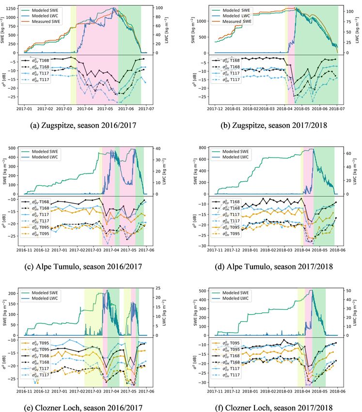
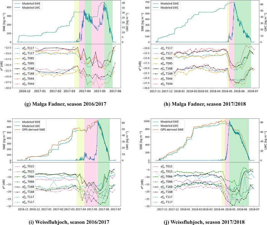
Figure 4 shows the time series of the backscattering coef-
ficient against the measured and/or modeled SWE and LWC
for the five test sites during the hydrological years 2016/2017
(left column) and 2017/2018 (right column). Yellow, red and
green areas highlight the moistening, ripening and runoff
phases respectively. These phases have been identified from
the SWE and LWC data according to Sect. 2.1. Specifically,
the moistening phase onset is identified by looking at the
liquid water content of the snowpack. We empirically estab-
lished a threshold of 1 kg m−2 that has to be satisfied for at
least 2 consecutive days. In other words, a significant melting In the following, for each of the five test sites, i.e.,
(and refreezing) cycle should be observed within 2 d. Among Zugspitze, Alpe del Tumulo, Clozner Loch, Malga Fadner
all the isolated moistening events, in this work we focus only and Weissfluhjoch, we will present the detailed comparison
on the moistening preceding a ripening phase. However, this
www.the-cryosphere.net/14/935/2020/ The Cryosphere, 14, 935–956, 2020944 C. Marin et al.: Use of Sentinel-1 to evaluate snowmelt dynamics in alpine regions
Figure 4.
of LWC, SWE and the S-1 σ 0 time series during the melting 4.1.1 Zugspitze
process. This will allow the derivation of important informa-
tion about the possibility to identify the three melting phases For this station, SWE was both measured and simulated,
in general. In the next section, the outcome of this compari- and LWC was simulated with SNOWPACK. The tempo-
son will be exploited to describe the characteristic behavior ral evolution of SWE measured by the snow scale and the
of the multitemporal SAR signal during the melting process. one simulated with SNOWPACK shows a good agreement.
For this station, the tracks T168 (descending, morning) and
T117 (ascending, afternoon) are available. The local inci-
The Cryosphere, 14, 935–956, 2020 www.the-cryosphere.net/14/935/2020/C. Marin et al.: Use of Sentinel-1 to evaluate snowmelt dynamics in alpine regions 945 Figure 4. Temporal evolution of the coefficient of backscattering acquired over the five test sites compared to LWC and SWE measured in situ at the stations (when available) and modeled with SNOWPACK (contains modified Copernicus Sentinel data, 2016/2018, processed by Eurac Research). The three phases during the melting have been identified from the in situ/modeled data. The first phase of moistening is reported in light yellow, the ripening phase in light red and the runoff in light green. For all the test sites we found that the multitemporal SAR measurements confirm the identification of the three melting phases. In particular, we systematically found that the SAR backscattering decreases as soon the snow starts containing water and increases as soon as SWE starts decreasing, which corresponds to the release of meltwater from the snowpack. dence angle for the two tracks differs by about 1◦ . For the pack metamorphism, snow stratification and the meteorolog- hydrological year 2016/2017 the backscattering remains al- ical conditions. Since the ripening phase is characterized by most constant during the accumulation phase until the begin- an increase in the LWC, the time series of the backscattering ning of the moistening phase (Fig. 4a). Here, as described in presents a decreasing trend. Interestingly, the minimum of Sect. 2.2, the increase in the LWC is accompanied by a de- σ 0 is reached at the end of the ripening phase and the begin- crease in the backscattering from −8.5 and −12.7 to −14.3 ning of the runoff phase, i.e., 20 May 2017. The runoff is in- and −20.0 dB for respectively VV and VH polarizations of stead characterized by a monotonic increase in the backscat- the afternoon track T117 between 19 and 25 March 2017 tering until all snow is melted. This characteristic behavior and from −5.8 and −12.7 to −12.5 and −18.1 dB for re- can be interpreted as follows: when the considered snowpack spectively VV and VH of the morning track T168 between reaches its saturation condition in terms of the LWC, snow 27 March and 4 April. The difference in the dropping of the density and internal structure, the backscattering recorded in signal acquired by the morning and afternoon track is due to the C band reaches its minimum value. These snowpack con- the diurnal melting and refreezing cycles. After this phase, ditions seem to represent the isothermal condition before the the ripening phase began with oscillations of the backscat- release of meltwater, i.e., the end of the ripening phase. After tering coefficient which on average presented low values. As the saturation point is reached, the monotonic increase in σ 0 described in Sect. 2.2 the oscillations are due to the snow- could be explained by a dominance of the superficial scatter- www.the-cryosphere.net/14/935/2020/ The Cryosphere, 14, 935–956, 2020
946                                      C. Marin et al.: Use of Sentinel-1 to evaluate snowmelt dynamics in alpine regions

ing that becomes more and more prominent due to a mono-            three tracks (T095 and T168, descending, and T117, ascend-
tonic increase in the LWC per volume (see Sect. 2.2). This         ing) acquired with different LIAs show very similar trends.
behavior continues until the snow disappears. This period
corresponds to the runoff formation phase, when SWE starts         4.1.3   Clozner Loch
decreasing. In Sect. 4.2 we will discuss a possible explana-
tion of this behavior. Regarding the winter 2017/2018 similar      For this station, the information about the LWC and SWE
observations were made, but here the snow ripening phase           was simulated with the SNOWPACK model. The calibra-
was limited to a very short period and the runoff started very     tion of the model was performed in order to achieve a high
early in mid-April due to strong insolation and high mean          agreement in terms of snow height and snow temperature
daily temperatures up to 5 ◦ C the days before. Interestingly,     (see Table 3). The tracks T168 (descending, morning), T117
during the runoff phase, σ 0 started increasing as expected,       (ascending, afternoon) and T095 (descending, morning) are
then it decreased due to a snow fall (probably wet) followed       available for this station. The LIAs for the three tracks are
by a relatively colder period which lasted some days at the        43, 36 and 39◦ , respectively.
end of May 2018, and finally it increased again until the end         The season 2016/2017 is characterized by two melting
of the snow season (Fig. 4b).                                      phases (Fig. 4e). In fact, the snow was completely melted in
   It is worth noting that the two polarizations acquired by       the first half of April with a new fresh snowfall at the end of
S-1 provided coherent information. However, few cases in           the month. For this reason, we highlighted the moistening–
which there is a depolarization of the signal can be spot-         ripening–runoff snowpack alteration sequence two different
ted during the ripening phase. Here the repeated cycles of         times. Interestingly, the time series of the backscattering
melting and refreezing can generate ice layers (Kattelmann         seems to properly follow the two melting processes with two
and Dozier, 1999), which affect the polarization in different      characteristic U-shaped behaviors. The melting process for
ways.                                                              the season 2017/2018 was more linear (Fig. 4f), and the σ 0
                                                                   time series of the three tracks provides coherent information
                                                                   with the one extracted by analyzing the time series of LWC
4.1.2   Alpe del Tumulo
                                                                   and SWE.

For this station, the information about the LWC and SWE            4.1.4   Malga Fadner
was derived through SNOWPACK. The calibration of the
model was performed in order to achieve a high agreement           For this station, the information about the LWC and SWE
in terms of snow height and snow temperature (see Table 3).        was derived through the SNOWPACK model. The calibra-
For this station, the tracks T168 (descending, morning), T117      tion of the model was performed in order to achieve a high
(ascending, afternoon) and T095 (descending, morning) are          agreement in terms of snow height and snow temperature
available. The LIAs for the three tracks are 40, 35 and 47◦ ,      (see Table 3). Four tracks are available for this station: T168
respectively.                                                      (descending, morning), T117 (ascending, afternoon), T044
   A very short moistening phase can be identified in both         (ascending, afternoon) and T095 (descending, morning). The
years from the modeled LWC and SWE time series (Fig. 4c,           LIAs for the three tracks are 46, 48, 38 and 34◦ , respectively.
d). These phases are well identified in the σ 0 time series by        The trend of the melting process over the two seasons
a drop of the morning and afternoon signal. The situation of       looks similar to Alpe del Tumulo. The season 2016/2017 is
the runoff phase 2016/2017 looks similar to Zugspitze for the      characterized by a consistent snowfall, which happened after
season 2017/2018: from the LWC and SWE time series two             an initial runoff phase of the snowpack. This together with
modes are visible, suggesting that the runoff was stopped by       a cold period stopped the process, which was resumed in
a cold period (with a new snowfall). This situation is reflected   May (Fig. 4g). The time series of the four tracks recorded
in the time series of the S-1 backscattering by the two char-      by S-1 backscattering showed two characteristic U-shaped
acteristic U-shaped behaviors indicating that a first runoff       behaviors indicating that a first runoff started after the first
started after the first minimum of σ 0 and continued for some      minimum of σ 0 and continued for some days following the
days following the monotonic increase in σ 0 , but then the        monotonic increase in σ 0 , but then the process was stopped
process was stopped by a new wet snowfall that forced the          by a new wet snowfall that forced the backscattering again
backscattering to a new minimum. Finally, the runoff phase         to the minimum. Nonetheless, the timings are different from
restarted, and the SAR signal increased again. However, the        the one identified with the modeled data of LWC and SWE.
runoff phases identified from the SAR local minima seem to         The strong depolarization may indicate a complex structure
be anticipated by about 2 weeks with respect to the modeling       of the snowpack with different ice layers. The melting pro-
results. Regarding the season 2017/2018, the runoff phase          cess for the season 2017/2018 was more linear, and the σ 0
showed a more linear behavior which is represented by the          time series of the four tracks provides coherent information
characteristic shape of σ 0 time series as the one identified      with the one extracted by analyzing the time series of LWC
in the Zugspitze test site. Finally, it is worth noting that the   and SWE (Fig. 4e).

The Cryosphere, 14, 935–956, 2020                                                       www.the-cryosphere.net/14/935/2020/
C. Marin et al.: Use of Sentinel-1 to evaluate snowmelt dynamics in alpine regions 947
Figure 5. Schematic representation of the evolution of the backscattering coefficient acquired in the morning (green line) and in the afternoon
(blue line) compared with LWC (yellow line) and SWE (red line) evolution. The offset between the morning and afternoon signals is due to
the generally different local incidence angle of the ascending and descending acquisitions in mountainous regions. The three melting phases
are identified from the LWC and SWE information. Correspondingly, the rules for the identification of each phase from the time series of
σ 0 are highlighted: a decrease of at least T (dB) from the mean value in dry snow conditions applied to the afternoon and morning signals
identifies the moistening and ripening onsets respectively. The local minima of the signals indicate the runoff onset.
4.1.5 Weissfluhjoch 4.2 Temporal evolution of the backscattering
For this station, the information about the LWC and SWE From the comparison carried out in the previous section and
was simulated with SNOWPACK; in addition, SWE GPS- by taking into account the main backscattering mechanisms
derived measurements were available. The calibration of the described in Sect. 2.2, it is possible to derive and explain the
model was performed in order to achieve a high agreement temporal behavior of σ 0 generated by a C-band SAR over
in terms of snow height and SWE (see Table 3). The tracks a sufficiently deep snowpack located in an open space that
T168 (descending, morning), T117 (ascending, afternoon), presents a linear transition between the three melting phases.
T015 (ascending, afternoon) and T066 (descending, morn- By analyzing the backscattering time series of the same pixel,
ing) are available for this station. The LIAs for the three the contribution of the LIA is always the same, making the
tracks are 41, 33, 43 and 31◦ , respectively. values of the time series comparable. Figure 5 shows an il-
The season 2016/2017 is characterized by an initial moist- lustrative evolution of σ 0 for a complete hydrological year
ening phase, followed by a ripening phase that was delayed that summarizes both the state-of-the-art background and the
by a cold period, when the LWC decreases almost to 0 observations done on real data. As described later, this con-
(Fig. 4i). In the middle of May a runoff phase started. The ceptual time signature will allow us to derive a set of rules
backscattering followed the different phases as expected. The for the identification of the melting phases also in time series
season 2017/2018 is more regular, with a monotonic increas- of backscattering never observed before or in independent
ing of LWC indicating a short moistening followed by a reg- datasets (e.g., Veyssière et al., 2018; Lievens et al., 2019).
ular ripening and the runoff. In this case the measured SWE Before the snow cover the terrain σ 0 is influenced by the
anticipated the runoff onset of about 1 week with respect to fluctuation of the soil moisture (Ulaby et al., 1996). Then,
the modeled SWE, which seems more in accordance with generally the first snow fall is wet or it covers relatively
the S-1 data. The backscattering shows a similar behavior of warm terrain, resulting in a wet snowpack. This generates
other previously discussed cases with the characteristic U- low backscattering values in the SAR response. This situ-
shaped signal except for the T066 that present several oscil- ation, which in alpine environments usually lasts for short
lations in the VH polarization. periods, ends either with a significant decrease in the tem-
perature that brings the snowpack to a dry condition or with
a complete melting of the snowpack. It is also possible that
the soil freezes before the first snowfalls. In this case the co-
www.the-cryosphere.net/14/935/2020/ The Cryosphere, 14, 935–956, 2020948 C. Marin et al.: Use of Sentinel-1 to evaluate snowmelt dynamics in alpine regions efficient of backscattering decreases and stabilizes around a respect to the general winter trend. This threshold has been given value not being affected by the soil moisture anymore. successfully used in Nagler et al. (2016) for detecting wet As soon as the snowpack starts incorporating liquid wa- snow from S-1 images. As soon as the time series of morning ter, the melting period starts. It can be divided into three backscattering also decreases by 2 dB or more, the ripening important phases as described in Sect. 2.1, i.e., the moist- phase begins. This phase, characterized by several oscilla- ening, the ripening and the runoff phases. The first phase tions, ends when both the morning and afternoon σ 0 values is related to the initial moistening of the snowpack. As dis- reach their local minimum. We propose the mean date among cussed previously, the liquid water is introduced in the snow the local minima as the start of the runoff phase, which is by rain and/or melt due to temperature and the incoming characterized by a monotonic increase in the coefficient of flux of shortwave radiation. At the beginning of the process backscattering. These rules are summarized in Algorithm 2. the value of LWC is low and therefore the SAR backscat- It is worth noting that the rules are not calibrated on the ob- tering experiences a relevant decrease in its value since the servations done in Sect. 4.1, but reflect the literature back- volumetric scattering dominates the total backscattering. The ground. drop of the signal is recognizable by imposing a given thresh- old T . During the moistening, the wetting front may be visi- ble only during the afternoon and not in the morning since the snowpack is still subjected to the diurnal cycles of melting and refreezing. As soon as the wetting front has penetrated the superficial insulating layer of the snowpack, the wet snow becomes visible also in the SAR early morning acquisitions. Please note that the systematic offset between the morning and afternoon signals represents the generally different local incidence angle of the ascending and descending acquisitions in mountainous region. At this point the phase of snowpack ripening starts. In this phase, the wetting front keeps pene- trating the snowpack conducting it to an isothermal condi- tion. During the ripening phase, which is influenced by the weather and the snowpack conditions, σ 0 varies according to the snow conditions but with an overall decreasing trend due to the increase in LWC. We observed that the minimum of σ 0 is reached at the end of the ripening phase and the beginning of the runoff phase for all the 10 time series observed (see Sect. 5). The runoff is instead characterized by a monotonic increase in the backscattering until all the snow is melted. To our knowl- edge, this characteristic behavior has never been observed in the literature before. Our interpretation is as follows: when the considered snowpack reaches its saturation condi- tion in terms of LWC and snow structure, the backscatter- ing recorded in the C band reaches its minimum value. This snowpack condition seems to correspond with the isothermal condition, i.e., the end of the ripening phase. After the satura- tion point is reached, the monotonic increase in σ 0 could be explained by one or the combination of the following factors: (i) an increase in the superficial roughness; (ii) a change in the snow structure, i.e., increase in the density and increase in grain size; and (iii) at the end of the melting the presence of patchy snow creates a situation of mixed contribution in- In the next section we applied these simple sets of rules side the resolution cell of the SAR, and therefore a further in order to identify the melting phases for each of the five increase in the total backscattering is recorded. considered test sites. Moreover, the same rules are used to On the basis of this analysis, we propose here a simple identify the runoff onset for each SAR pixel in the topograph- set or rules to identify the snow melting phases on the ba- ically well defined catchment of the Zugspitzplatt obtaining sis of the multitemporal SAR signal. The start of the melting a spatially distributed map of the runoff timing. process can be identified by a decrease in the multitemporal SAR signal recorded in the afternoon of 2 dB or more with The Cryosphere, 14, 935–956, 2020 www.the-cryosphere.net/14/935/2020/
You can also read