Mapping pan-Arctic landfast sea ice stability using Sentinel-1 interferometry - The Cryosphere
←
→
Page content transcription
If your browser does not render page correctly, please read the page content below
The Cryosphere, 13, 557–577, 2019
https://doi.org/10.5194/tc-13-557-2019
© Author(s) 2019. This work is distributed under
the Creative Commons Attribution 4.0 License.

Mapping pan-Arctic landfast sea ice stability using
Sentinel-1 interferometry
Dyre O. Dammann1 , Leif E. B. Eriksson1 , Andrew R. Mahoney2 , Hajo Eicken3 , and Franz J. Meyer2
1 Department   of Space, Earth and Environment, Chalmers University of Technology, Gothenburg, 41296, Sweden
2 Geophysical   institute, University of Alaska Fairbanks, Fairbanks, 99775, USA
3 International Arctic Research Center, University of Alaska Fairbanks, Fairbanks, 99775, USA

Correspondence: Dyre O. Dammann (dyre.dammann@chalmers.se)

Received: 22 June 2018 – Discussion started: 11 July 2018
Revised: 23 December 2018 – Accepted: 19 January 2019 – Published: 18 February 2019

Abstract. Arctic landfast sea ice has undergone substantial         1     Introduction
changes in recent decades, affecting ice stability and includ-
ing potential impacts on ice travel by coastal populations          1.1    Landfast sea ice stability and stakeholder
and on industry ice roads. We present a novel approach for                 dependence
evaluating landfast sea ice stability on a pan-Arctic scale us-
ing Synthetic Aperture Radar Interferometry (InSAR). Us-            Sea ice is an important component of Arctic ecosystems and
ing Sentinel-1 images from spring 2017, we discriminate be-         provides important functions as a climate regulator (Screen
tween bottomfast, stabilized, and nonstabilized landfast ice        and Simmonds, 2010), habitat for marine biota (Thomas,
over the main marginal seas of the Arctic Ocean (Beau-              2017), and a platform for coastal populations (Krupnik et
fort, Chukchi, East Siberian, Laptev, and Kara seas). This          al., 2010). During the last century, an expansion of trans-
approach draws on the evaluation of relative changes in in-         portation and resource extraction have led to increased hu-
terferometric fringe patterns. This first comprehensive as-         man presence in the Arctic and further diversification of ice
sessment of Arctic bottomfast sea ice extent has revealed           use (Eicken et al., 2009). The recent retreat of sea ice ob-
that most of the bottomfast sea ice is situated around river        served over the past several decades (Stroeve et al., 2012;
mouths and coastal shallows. The Laptev and East Siberian           Comiso and Hall, 2014; Meier et al., 2014) has already
seas dominate the aerial extent, covering roughly 4100 and          resulted in widespread consequences for ice users (ACIA,
5100 km2 , respectively. These seas also contain the largest        2004; Aporta and Higgs, 2005; Fienup-Riordan and Rear-
extent of stabilized and nonstabilized landfast ice, but are        den, 2010; Orviku et al., 2011; Druckenmiller et al., 2013),
subject to the largest uncertainties surrounding the mapping        as well as increasing hazards (Ford et al., 2008; Eicken and
scheme. Even so, we demonstrate the potential for using In-         Mahoney, 2015). At the same time, the related increased ac-
SAR for assessing the stability of landfast ice in several key      cessibility to Arctic waters (Stephenson et al., 2011) is lead-
regions around the Arctic, providing a new understanding of         ing to more ship traffic and resource exploration (Lovecraft
how stability may vary between regions. InSAR-derived sta-          and Eicken, 2011; Eguíluz et al., 2016). It is further recog-
bility may serve for strategic planning and tactical decision       nized that sea ice conditions for future Arctic marine opera-
support for different uses of coastal ice. In a case study of the   tions will be challenging, and will require substantial mon-
Nares Strait, we demonstrate that interferograms may reveal         itoring and improved observations (Arctic Council, 2009).
early-warning signals for the breakup of stationary sea ice.        This improvement will require observations on local and re-
                                                                    gional scales in order to provide an assessment of environ-
                                                                    mental hazards and effective emergency responses (Eicken
                                                                    et al., 2011).
                                                                       Most of the Arctic Ocean is dominated by drifting pack
                                                                    ice, whereas stationary landfast ice occupies much of the

Published by Copernicus Publications on behalf of the European Geosciences Union.
558                                                       D. O. Dammann et al.: Mapping pan-Arctic landfast sea ice stability

Figure 1. (a) October–March (freeze-up) and (b) April–September (breakup) monthly mean landfast sea ice extent (1976–2007), derived
from sea ice charts based on optical instruments and SAR. The data for this figure were obtained from the National Snow and Ice Data Center
(Yu et al., 2014).

Arctic coastlines roughly between November and June, de-                al., 2008; Stevens et al., 2010). This bottomfast ice allows
pending on location (Fig. 1; Yu et al., 2014). Sections of land-        for heat loss from the seafloor and is therefore an integral part
fast ice, often from several kilometers to hundreds of kilome-          of aggregating and maintaining subsea permafrost (Solomon
ters wide, are held in place by grounded ridges, islands, or            et al., 2008; Stevens et al., 2008, 2010; Stevens, 2011), as
coastline morphology, such as embayments or fjords. Sim-                well as controlling coastal stability and morphology (Are and
ilar to drifting pack ice, landfast ice has declined signifi-           Reimnitz, 2000; Eicken et al., 2005). Bottomfast ice is also
cantly during the last few decades, particularly in terms of            relevant for fish, as it reduces habitable shallow waters dur-
delayed freeze-up in the Beaufort (Mahoney et al., 2014)                ing winter (Hirose et al., 2008), and for on-ice operations,
and Laptev (Selyuzhenok et al., 2015) seas, as well as to a             as it can support a much larger load than floating ice. High
significantly reduced extent in the Chukchi Sea (Mahoney                to moderately stable landfast ice is of relevance to industrial
et al., 2014). Later freeze-up critically impacts stakeholders          (Potter et al., 1981) and subsistence ice use (Druckenmiller
through reduced stability of landfast ice in response to fewer          et al., 2013), as well as for habitats (Tibbles et al., 2018).
grounded ridges capable of withstanding wind, ocean, or ice             Ringed seals, for instance, are dependent on stable land-
forcing (Dammann, 2017). Previous research suggests that                fast ice for denning (Smith, 1980). Low-stability ice is po-
landfast ice stability can be expressed in terms of combined            tentially relevant for ocean-based operations, such as ship-
frictional resistance provided by relevant grounding or at-             ping through trans-Arctic passages close to the coast, where
tachment points (e.g., islands and grounded ridges; Mahoney             patches of landfast ice occasionally break off and drift into
et al., 2007; Druckenmiller, 2011). Although landfast ice is            nearby shipping lanes, potentially causing hazards. Even ar-
stationary, it deforms at the centimeter to meter scale, on             eas hundreds of kilometers from landfast ice can be impacted
timescales of days to months due to forcing from wind, cur-             through the failure of ice arches.
rents, and drifting ice (Dammann et al., 2016). Its stability              Ice arches may be considered an additional zone of “tem-
in part determines the rate at which the ice deforms, and ulti-         porarily stabilized pack ice”. Ice arches form when ice mov-
mately, the severity of breakout events or magnitude of struc-          ing through a narrow passage experiences flow stoppage as a
tural defects. We suggest that landfast sea ice can be further          result of confining pressure and begins to behave like landfast
categorized into three regimes, defined through their respec-           ice, though potentially without cohesive strength between in-
tive stabilities: (1) bottomfast ice, (2) floating ice enclosed         dividual floes (Hibler et al., 2006). Ice arches typically form
in lagoons or fjords, or sheltered by point features such as            between November and March (Moore and McNeil, 2018),
grounded ridges or islands, and (3) floating ice extensions             and can block the export of ice through straits as wide as
(Table 1). A typical landfast ice regime is illustrated in Fig. 2,      100 km (Melling, 2002). When formed, such arches repre-
where the stability of the landfast ice area decreases from the         sent a significant obstacle to marine traffic, due to the high
coast toward the open ocean (Dammann et al., 2016).                     confining pressures that make icebreaking impossible for all
   Bottomfast sea ice can grow laterally to kilometer scale             but the most powerful vessels. Arches can in some locations
during winter, depending on local bathymetry (Solomon et                prevail into the following season (Melling, 2002), but typ-

The Cryosphere, 13, 557–577, 2019                                                              www.the-cryosphere.net/13/557/2019/
D. O. Dammann et al.: Mapping pan-Arctic landfast sea ice stability                                                                  559

Figure 2. Conceptual scheme of landfast sea ice, where different regimes possess different levels of stability.

ically collapse in July–August (Kwok, 2005). Conversely,                  fast sea ice, typically derived by evaluating unchanged sec-
their breakup can lead to the advection of large amounts of               tions of ice between consecutive SAR backscatter scenes
thick multiyear ice into high-traffic shipping routes (Barber             (Johannessen et al., 2006; Giles et al., 2008; Mahoney et
et al., 2018), creating a well-known hazard (Bailey, 1957;                al., 2014). In addition to its use in the mapping of landfast
Wilson et al., 2004; Howell et al., 2013). Recent and ongo-               ice, SAR backscatter can also discriminate between multi-
ing sea ice decline is leading to an increasing presence of               year and first-year ice (Onstott, 1992) and identify different
thinner ice in the Canadian Archipelago (Haas and Howell,                 roughness regimes (Dammann et al., 2017). SAR has also
2015), and weaker ice due to warmer temperatures (Melling,                been used to estimate the advection of ice through straits
2002) may lead to earlier breaching of ice arches. This could             in the Canadian Archipelago (Melling, 2002; Kwok, 2006;
result in a larger amount of advected ice with potentially                Howell et al., 2013). However, SAR backscatter typically
longer travel paths, increasing the severity of such events               does not give information pertaining to the stability of land-
(Melling, 2002; Barber et al., 2018). One location of partic-             fast ice or temporarily stabilized pack ice, since the internal
ular interest is the Nares Strait, situated between Greenland             movement of the landfast ice is too small (mm day−1 ) to be
and Ellesmere Island, featuring a seasonal ice arch (Kwok,                identified with change detection.
2005; Kwok et al., 2010) with important implications for the                 SAR interferometry (InSAR) is a signal-processing tech-
multiyear ice budget of the Arctic Ocean (Kwok et al., 2010).             nique, which extracts the phase difference between two SAR
This stability is also relevant for destinational cargo shipping          images acquired with similar viewing geometries. This phase
in the Arctic, as less stable, thinner ice is easier to break             difference (typically referred to as interferometric phase)
through, resulting in opportunities for docking in areas of               can either signify topography if acquisitions are separated
landfast ice. For navigating through landfast ice, stabiliza-             in space (i.e., nonzero perpendicular baseline) or measure
tion through ridging is also important to identify, as ridges             the line-of-sight motion if acquisitions are separated in time
can be problematic to navigate and are often associated with              (nonzero temporal baseline; Bamler and Hartl, 1998; Ferretti
hazards (Hui et al., 2017).                                               et al., 2007). InSAR has been successfully used to map land-
                                                                          fast ice edges by identifying areas of slow motion (Meyer et
1.2   Remote sensing of landfast ice stability                            al., 2011). InSAR has also provided information pertaining
                                                                          to landfast ice dynamics (Li et al., 1996; Morris et al., 1999;
Satellite remote sensing is an important tool for measuring               Vincent et al., 2004; Marbouti et al., 2017) and topogra-
ice conditions in the Arctic, including the mapping of land-              phy (Dammann et al., 2017; Dierking et al., 2017) by eval-
fast ice (Muckenhuber and Sandven, 2017). Optical and ther-               uating the phase change between acquisitions. InSAR has
mal satellite data, such as from the Advanced Very High Res-              also been shown to reveal plausible rheologies for landfast
olution Radiometer (AVHRR), were used to produce opera-                   ice (Dammert et al., 1998) and has been used to determine
tional ice charts until the early 1990s, when SAR was in-                 the origin of internal ice stresses (Berg et al., 2015). Com-
troduced into the charting production (Yu et al., 2014) as                bined with inverse modeling, InSAR enables us to determine
a superior data set, thanks to its independence from light                ice deformation modes (Dammann et al., 2016), rates, and
and weather conditions and its higher (∼ 100 m) resolution                the associated stress and fracture potentials (Dammann et
– both advantageous to stakeholders (Eicken et al., 2011).                al., 2018b).
Different techniques exist to map the boundaries of land-

www.the-cryosphere.net/13/557/2019/                                                                 The Cryosphere, 13, 557–577, 2019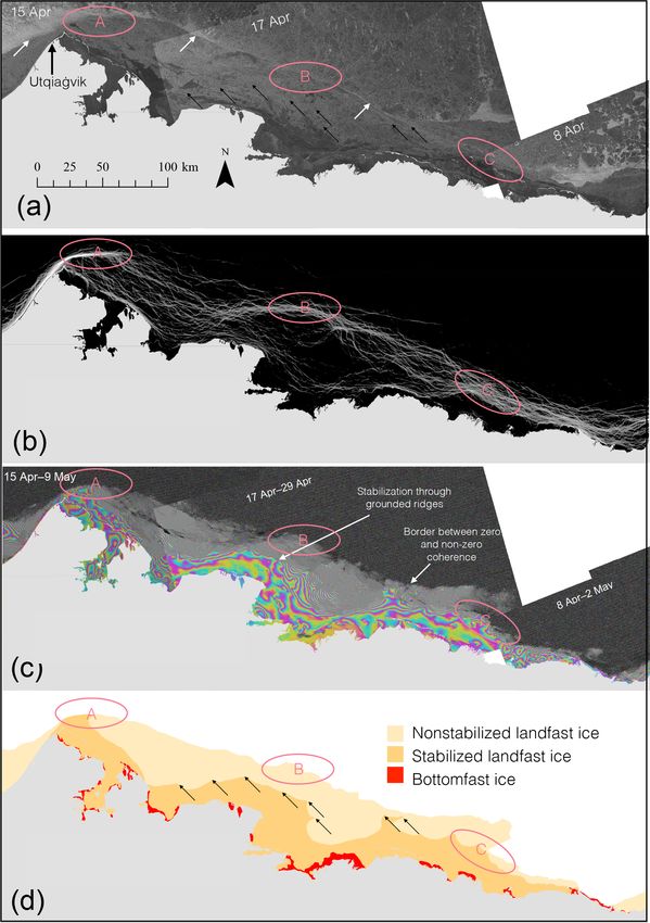
560                                                     D. O. Dammann et al.: Mapping pan-Arctic landfast sea ice stability

   These studies have demonstrated (1) the potential of In-        there is significant change in the scattering medium (Meyer
SAR as a tool for assessing landfast ice dynamics and stabil-      et al., 2011).
ity through local case studies and (2) its utility as a planning
tool for on-ice operations (Dammann et al., 2018a, b). They        2.2   Sentinel-1 data
have also laid the foundation for applying InSAR on a larger
scale, potentially as a means for generating operational infor-    This study uses Sentinel-1, a constellation of two C-band
mation products and evaluating long-term trends. The cover-        SAR systems (Sentinel-1A and B) in operation since 2014
age and access to InSAR-compatible SAR scenes has been             and 2016, with a repeat-pass interval of 6 to 12 days, depend-
an obstacle in the past, but has improved significantly since      ing on whether both or just one of the satellites acquire data.
the launch of Sentinel-1 (the suitability of Sentinel-1 for au-    Thanks to a free-and-open data policy and large spatial cov-
tomatic SAR processing has been shown, e.g., in Meyer et           erage, we obtained Sentinel-1 acquisitions for five marginal
al., 2015). In this study, we explore InSAR as a tool for pro-     seas of the Arctic Ocean, enabling mapping of landfast sea
viding pan-Arctic information on ice stability, which is rel-      ice on a pan-Arctic scale. All images used were captured
evant to subsea permafrost, biological habitats, and sea ice       in interferometric wideswath (IW) mode, with a single-look
use. The goal of this work is to determine Sentinel-1 in-          resolution of roughly 3 m × 22 m in slant range and azimuth,
terferometric data availability along substantial parts of the     and a ∼ 250 km swath width. Images were acquired almost
circumpolar coastlines and to explore their applicability for      exclusively between March and May 2017 (see Supplement
consistently mapping landfast sea ice stability zones in dif-      for full list of images used). We acquired over 100 SAR im-
ferent geographic regions. We further explore the limitations      ages, covering nearly the entire continental coastlines of the
of the technology and possible applications.                       Beaufort, Chukchi, East Siberian, Laptev, and Kara seas. To
                                                                   reduce computational costs, we omitted Greenland, some is-
                                                                   land groups, and the Canadian Archipelago, which are char-
                                                                   acterized by extensive coastline lengths. In this work, we fo-
2     Data and methods                                             cused on the Alaska and Russian marginal seas of the Arctic
                                                                   Ocean. These coastlines have high economic significance for
2.1    InSAR principles                                            the shipping and natural resource industries, and also feature
                                                                   dynamically diverse ice regimes. Large areas of bottomfast
The interferometric phase may be related to lateral (e.g.,         ice are expected in these regions. Except for one approxi-
thermal contraction or displacement due to compressional           mately 50 km long section of coast in the Kara Sea and the
or shear forces) or vertical (e.g., through buckling or tidal      eastern Laptev Sea, multiple InSAR compatible pairs were
displacement) sea ice motion that occurs in between the ac-        available for the specified time frame. This allowed us to se-
quisition times for the two SAR images. A phase signature          lect interferograms centered around the end of April, when
can sometimes also be attributed to factors not related to sur-    most Arctic landfast ice is at its maximum extent and thick-
face motion, such as atmospheric phase delay. Of the phase         ness.
change attributed to motion, only displacement in line-of-            In addition to images obtained for the large-scale map-
sight direction (1rLOS ) results in a phase change 18disp ,        ping of stability zones, a series of six consecutive image pairs
according to 18disp = 4π 1rLOS /λ. The observed phase is           were acquired covering the Nares Strait and the breakup of
measured within the wrapped interval of [0; 2π [. The inter-       an ice arch during spring 2017. This image sequence featured
ferogram is a series of fringes representing the projection of     a 6-day temporal baseline covering a time span of 36 days.
the true three-dimensional ice motion onto the line-of-sight
vector. The orientation of fringes can be used to interpret the    2.3   Data processing
direction of the three-dimensional motion field, and fringe
spacing is an indicator of the deformation rate. The interpre-     All the complex Sentinel-1 data were processed to obtain
tation of observed fringe patterns is, however, not straight-      backscatter in order to visually interpret features (e.g., land-
forward, and it typically requires the use of an inverse model     fast ice edge, fracturing, ice roughness and types). Data were
(Dammann et al., 2016). The interferometric phase values           further processed for interferometry. Depending on the per-
will only be useful if scattering elements remain largely un-      pendicular baseline, sea ice topography can have a modest
changed throughout the time interval bracketed by the im-          impact on the phase difference. Due to tight baseline limits
age pairs used in processing. InSAR phase stability, referred      (∼ 50 m standard deviation) for the Sentinel-1 constellation,
to as InSAR coherence, depends largely on topography cou-          and since sea ice topography rarely exceeds 10 m, impacts for
pled with a perpendicular baseline, as well as the temporal        interferogram interpretation are minimal for the data shown
stability of the scatterers on the ground surface. Coherence       here. In this work we predominately employed acquisitions
ranges between 0 (pure noise) and 1 (no noise), and serves         with a temporal lag of either 12 or 24 days, depending on data
as a measure of the quality of the interferogram. Coherence        availability. For this timespan, the coherence over landfast ice
is generally high if scatterers remain unchanged and low if        was found to be generally high, due to its stationary nature.

The Cryosphere, 13, 557–577, 2019                                                       www.the-cryosphere.net/13/557/2019/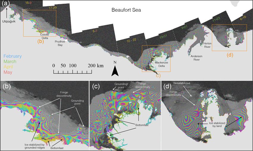
D. O. Dammann et al.: Mapping pan-Arctic landfast sea ice stability                                                            561

However, coherence loss was evident in some areas – in par-        map three different zones of relative stability: bottomfast ice,
ticular in the Chukchi Sea, such as in the Kotzebue Sound.         stabilized ice, and nonstabilized ice (Table 1). These three
This was likely predominately due to surface melt, as air          zones are subjectively and manually mapped without the use
temperature reached above freezing between SAR acquisi-            of specific threshold values.
tions. Other possible contributing reasons for coherence loss         Bottomfast ice is identified with near-zero phase change
in this region could include ice motion, subsurface ice thin-      in the interferogram. It can often be distinguished from adja-
ning from river runoff, and low signal-to-noise ratio. Signif-     cent floating ice commonly featuring a nonzero phase change
icant decorrelation can also occur in late spring, as the onset    or low coherence (Fig. 3a). The shoreward boundary of bot-
of melt causes substantial changes in the scattering medium.       tomfast ice is difficult to obtain from the interferogram alone,
In this work, we obtained images as close to late April as pos-    since the phase signatures over bottomfast ice and low-lying
sible. This time frame was found to be ideal for our purpose,      coastal areas are similar. The use of the landmask (Wessel
as ice thickness is near its maximum, leading to maximum           and Smith, 1996) is not ideal, since subtle coastal features
stability and minimizing impacts from the onset of melt. To        such as sediment bars are often not captured. We therefore
ensure a realistic representation of an operationally produced     delineated the coastline (i.e., shoreward boundary of bottom-
synoptic, contiguous pan-Arctic interferogram, we did not at-      fast ice) using the backscatter signature in a composite im-
tempt to derive alternative interferograms (i.e., different time   age with backscatter and phase (Fig. 3b). Plotting bottomfast
periods) in cases of low coherence.                                ice with the landmask can thus give the wrongful appearance
   All backscatter images and interferograms in this work          that (1) areas of near-zero phase should have been mapped as
were produced using a standard Sentinel-1 workflow in              bottomfast and (2) bottomfast ice appears in sporadic areas
Gamma software (Werner et al., 2000). The IW images ini-           along the coast separated by floating ice.
tially consist of independent bursts and swaths, which we             We could often identify stabilized ice by a stark fringe dis-
combined to utilize the full extent of the acquisition. We fur-    continuity between different fringe densities (Fig. 3c). How-
ther coregistered pairs of acquisitions to ensure images cover     ever, in some regions, changes in stability are more grad-
exactly the same area with subpixel accuracy. Images were          ual between zones (Figs. 6c and 7c). Mapping of such re-
then multilooked, averaging 10 pixels in range and 2 pix-          gions are therefore more subjective and possibly less exact.
els in azimuth, resulting in reduced speckle and a final pixel     In cases lacking stark fringe discontinuities, stabilized ice is
spacing of roughly 23 × 28 m. Next, spectral filtering was         also mapped in regions featuring a very slight phase response
performed to ensure both images comprise the same spec-            with no clear fringe patterns (Fig. 3d).
tral range, reducing phase noise in the final interferogram.          Nonstabilized ice is identified as landfast ice (i.e., areas
The interferometric phase was calculated for each pixel of         featuring relatively high interferometric coherence) other-
the coregistered and filtered images. Furthermore, the ex-         wise not marked as bottomfast or stabilized ice. Nonstabi-
pected phase ramp in cross-track direction from a station-         lized ice commonly features clear fringe patterns (Fig. 3e).
ary flat earth surface was removed. The phase noise of the
final interferogram was reduced using an adaptive phase fil-       2.5   Validation areas and data
ter (Goldstein and Werner, 1998). The result was 52 inter-
ferograms, covering almost the entire coastline between the        The Beaufort Sea coast of Alaska was used for validation, as
Canadian Archipelago and the Barents Sea.                          landfast sea ice in this area includes all three stability zones
                                                                   (bottomfast, stabilized, and nonstabilized), and ample valida-
2.4   Mapping landfast ice stability zones                         tion data are available from previous studies. Alaska’s Beau-
                                                                   fort Sea coast is of major interest in the context of local and
In this work, we evaluated relative ice stability based on         indigenous ice use, as well as industry resource exploration
fringe spacings within individual interferograms. This al-         and extraction. Some areas along this coastline feature simi-
lowed us to identify variations within an area imaged under        lar landfast ice extent over timescales from months to years.
largely the same conditions (e.g., close to the same wind and      It was found that these regions (“nodes”) of consistent land-
ocean forcing). Trends from higher to lower fringe density         fast ice extent are often tied to the location of the 20 m iso-
will likely correspond to increasing ice stability. Therefore,     bath, a water depth associated with the grounding of pressure
interferograms can provide information related to the spatial      ridges stabilizing the landfast ice (Mahoney et al., 2014). In-
variations in stability. Meyer et al. (2011) demonstrated that     digenous knowledge and a field study also indicate persis-
interferometry can be used to map the landfast ice based on        tent grounded ridges in the location of the node closest to
a coherent phase response. Their work also suggested that          Utqiaġvik, Alaska (Meyer et al., 2011). We also evaluated
fringe patterns are significantly impacted by grounded ridges      our results near Stolbovoy Island in the Laptev Sea. This area
and reduced fringe density. Dammann et al. (2018c) further         features a shoal of < 10 m water depth, leading to earlier for-
showed that bottomfast ice can be mapped based on a near-          mation of fast ice than the surrounding areas (Selyuzhenok
zero phase change where ice is frozen to the seafloor. We          et al., 2015), likely due to the formation of grounded ridges
built on this work by suggesting that InSAR can be used to         on the shoal and resulting in increased stability.

www.the-cryosphere.net/13/557/2019/                                                        The Cryosphere, 13, 557–577, 2019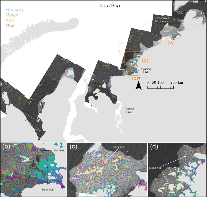
562 D. O. Dammann et al.: Mapping pan-Arctic landfast sea ice stability
Table 1. Landfast sea ice stability regimes and assigned stability zones identified using InSAR.
Landfast ice regime Stability Stability zone Identification
1. Bottomfast sea ice Completely stable. Ice is frozen to or Bottomfast No identifiable phase
(i.e., ice frozen to resting on the seafloor, restricting difference from the
or in broad contact lateral motion. Vertical tide jacking adjacent land
with the seafloor) may occur as the ice thickens.
2. Floating ice sheltered Moderate stability. Ice is supported by Stabilized Poorly defined, widely
by point features, coastlines or point features, completely spaced fringes, or abruptly
such as grounded ridges or largely inhibiting breakout events. reduced fringe spacing
or islands, or fully In addition to thermal creep, internal compared to offshore ice
enclosed in lagoons stress from more dynamic ice can
or fjords propagate in between pinning points,
resulting in decimeter to meter-scale
nonelastic deformation.
3. Floating ice extensions Low stability. Dominated by meter-scale Nonstabilized Well-defined fringe
deformation from ice, wind, and orientation or
ocean forcing. Persistent inelastic patterns
deformation can lead to accumulated
strain on the order of tens of meters
on timescales exceeding several
weeks. Ice may remain attached
(Mahoney et al., 2004) or can
break-off from the stabilized ice.
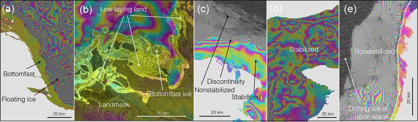
Figure 3. (a) Example of interferometric phase response over bottomfast ice. (b) Phase/backscatter composite near a delta. This example
exhibits a poor match between the landmask (transparent black shading) and low-lying coastal areas. Here, bottomfast ice (white outline)
had to be mapped against the coastline, as identified in the backscatter data. (c) Example of stabilized ice as identified based on a phase
discontinuity. (d) Example of stabilized ice as identified by low fringe density and nonconsistent fringe patterns. (e) Example of nonstabilized
ice as identified by high fringe density. Land is masked out in light gray in panels (a, c, d, e).
3 Results The landfast sea ice extent in the Beaufort Sea ranges from
almost zero up to 100 km (Fig. 4a). River outlets such as the
3.1 Evaluating landfast ice stability zones Colville and Mackenzie deltas feature extensive regions of
bottomfast ice several kilometers wide (Fig. 4b, c). Bottom-
We constructed a series of Sentinel-1 interferograms along fast ice is also prominent in many lagoons along the coast.
the coastlines of five marginal seas in the Arctic Ocean dur- Much of the floating ice along the coast from Prudhoe Bay
ing 2017: the Beaufort, Chukchi, East Siberian, Laptev, and to Point Barrow is stabilized. This stabilized ice can be iden-
Kara seas. As seen in the interferograms (Figs. 4–8), landfast tified by a stark fringe discontinuity separating regions of dif-
sea ice varies substantially between the seas in terms of the ferent fringe density and stability (Fig. 4a, b). The line of dis-
extent and interferometric fringe density. continuity features several seaward points, an expected pat-
The Cryosphere, 13, 557–577, 2019 www.the-cryosphere.net/13/557/2019/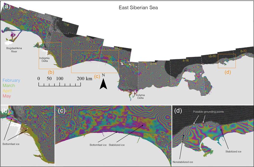
D. O. Dammann et al.: Mapping pan-Arctic landfast sea ice stability                                                                   563

Figure 4. (a) Sentinel-1 interferograms derived from image pairs acquired over the Beaufort Sea between March and May 2017. Numbers
on images represent date ranges. The colors blue, green, yellow, and red signify the months of February–May. (b, c, d) Three enlarged areas
identified in (a) are further discussed in the text.

tern surrounding grounded ridges. This is because grounded              of coastline even tens of kilometers away from major rivers,
ridges result in a shoreward increase in stability that does            though most of the bottomfast ice is situated near the Kolyma
not extend to areas immediately to the side of the ridges (the          and Indigirka deltas (Fig. 6b). In contrast to the Beaufort and
alongshore direction). Examples of likely grounding points              Chukchi seas, stabilized ice extends several tens of kilome-
are indicated with white arrows in Fig. 4b, and similar pat-            ters offshore without being sheltered by coastline morphol-
terns are also apparent near the Mackenzie Delta (Fig. 4c).             ogy or islands (Fig. 6c). These large areas also lack clear
The landfast ice in the eastern part of the Beaufort Sea also           indications of the presence of grounded ridges (Fig. 6d).
consists of large areas of stabilized ice. Here, the landfast ice          Landfast ice in the Laptev Sea, similar to the East Siberian
is noticeably sheltered by land features, resulting in lower-           Sea, extends upwards of 100 km from the shore (Fig. 7a).
density fringes (Fig. 4d).                                              Here, most of the bottomfast ice is situated around river out-
   Landfast sea ice in the Chukchi Sea is generally less ex-            lets and in particular near the Lena Delta, extending tens
tensive than in the Beaufort Sea, particularly along the Rus-           of kilometers from shore (Fig. 7b). This delta features a
sian coast (Fig. 5a). Bottomfast ice in the Chukchi is con-             large amount of small, low-lying land areas (e.g., gravel is-
strained mostly to lagoons. Some of these lagoons, such as              lands) only partly covered by the landmask. This has made
the Kasegaluk, consist almost exclusively of bottomfast ice             it problematic to delineate all areas of bottomfast ice and
(Fig. 5b). Only a few areas of landfast ice appear to be sta-           led to more approximate delineations than in the other deltas
bilized, including the northern coast of Alaska near Peard              mapped. On the east side of the Lena Delta and south of the
Bay (Fig. 5c) and the southern Chukchi Sea near Shishmaref              Great Lyakhovsky Island, there are extensive sections of sta-
(Fig. 5d). The Chukchi Sea consists predominantly of non-               bilized ice (Fig. 7c). Some regions of the eastern Laptev Sea
stabilized ice, with the most extensive region of landfast ice          lack a clear discontinuity, but at the same time feature locally
situated off the shore of the village of Shishmaref (Fig. 5d).          reduced fringe density, indicative of stabilized ice (Fig. 7c).
The Chukchi Sea features coherence loss in several regions              We also considered these areas to be stabilized (Fig. 7c),
such as the Kotzebue Sound (Fig. 5a).                                   though possibly as a result of different ice types or thick-
   The landfast ice in the East Siberian Sea is more extensive          nesses, rather than through grounding or sheltering. How-
than in the Chukchi and Beaufort seas and can extend over               ever, one offshore area is clearly identified as stable by a lack
100 km from the shore (Fig. 6a). Bottomfast ice is also more            of consistent fringe patterns and a clear discontinuity, likely
extensive than in the Beaufort and Chukchi seas. The bot-               due to grounded ridges (Fig. 7d).
tomfast ice in the East Siberian Sea follows several sections

www.the-cryosphere.net/13/557/2019/                                                              The Cryosphere, 13, 557–577, 2019
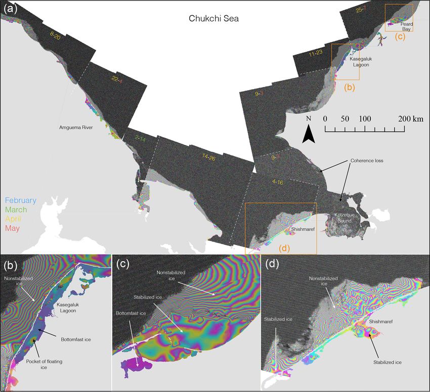
564                                                       D. O. Dammann et al.: Mapping pan-Arctic landfast sea ice stability

Figure 5. (a) Sentinel-1 interferograms derived from image pairs acquired over the Chukchi Sea between March and May 2017. Numbers
on images represent date ranges. The colors blue, green, yellow, and red signify the months of February–May. (b, c, d) Three enlarged areas
identified in (a) are further discussed in the text.

   Landfast ice in the Kara Sea features a much smaller ice                Most areas with extensive bottomfast ice reaching several
extent than the other Russian seas (Fig. 8a). Bottomfast ice is         kilometers from shore are located either in the vicinity of
also much less prevalent and largely situated near the Pyasina          river deltas or within lagoons. The East Siberian Sea and
River (Fig. 8b). The landfast ice extends tens of kilometers            its three large river systems (the Indigirka, Bogdashkina, and
from shore, predominately in areas supported by offshore is-            Kolyma rivers) contain the most bottomfast ice of the regions
lands and archipelagos (Fig. 8c, d). In these archipelagos, the         considered here. The Laptev Sea also contains a large area of
ice confined by islands is largely stabilized (Fig. 8c).                bottomfast sea ice. Together, the Laptev and East Siberian
   Interferograms have enabled the mapping of landfast ice              seas contain over half (∼ 57 %) of the total areal extent of
stability zones based on subjective interpretations of inter-           bottomfast ice calculated, while the Chukchi Sea features
ferometric fringes (Fig. 9). The resulting stability map allows         the lowest extent of bottomfast ice of the regions considered
for a large-scale comparison and analysis of bottomfast, sta-           here. Bottomfast ice is predominately situated in lagoons.
bilized, and nonstabilized landfast ice, within and between                Stabilized ice was found in all marginal seas (Fig. 9),
the different seas. For this comparison, we have calculated             though its relative contributions to overall landfast ice extent
the area of each stability zone (Table 2). However, it is im-           varied widely. The largest extent of stabilized landfast ice in
portant to note these area calculations are not complete, as            our study region was found in the Laptev and East Siberian
the analysis omitted some island groups and included some               seas. These regions feature particularly large continuous ar-
data gaps.                                                              eas of stabilized ice labeled A–F in Fig. 9. Even so, as we

The Cryosphere, 13, 557–577, 2019                                                              www.the-cryosphere.net/13/557/2019/
D. O. Dammann et al.: Mapping pan-Arctic landfast sea ice stability                                                                                             565

Figure 6. (a) Sentinel-1 interferograms derived from image pairs acquired over the East Siberian Sea between March and May, 2017.
Numbers on images represent date ranges. The colors blue, green, yellow, and red signify the months of February–May. (b, c, d) Three
enlarged areas identified in (a) are further discussed in the text.

Table 2. Approximate area coverage of landfast ice (in thousand km2 ).

                 Area                       Bottomfast         Stabilized       Nonstabilized          Total area of                  Area fraction:
                                                                                                        landfast ice        nonstabilized/stabilized
                 Beaufort Sea                    2.5                    35                     29                  67                                0.83
                 Chukchi Sea                     1.8                    4.6                    25                  31                                5.43
                 East Siberian Sea               5.1                     45                    80                 130                                1.78
                 Laptev Sea                      4.1                    74                    127                 205                                1.72
                 Kara Sea                        2.6                    16                     37                  56                                 2.3
               The bottomfast ice zone is constrained between its outer extent (interpreted from the phase) and the coast (as interpreted from the
               backscatter scenes). The stabilized zone is constrained between its outer extent (as interpreted from the phase) and the bottomfast ice or the
               landmask (Wessel and Smith, 1996). The nonstabilized ice is constrained between the outer extent of nonzero coherence and the bottomfast
               ice, stabilized ice, or the landmask.

delineated here, the Beaufort Sea is the only sea that features                             In the Chukchi Sea, we identified the vast majority of
more stabilized ice than nonstabilized ice. This is likely at-                           landfast ice as nonstabilized (Fig. 9), resulting in our largest
tributed to the large grounded sections, as well as areas shel-                          areal fraction (nonstabilized ice vs. stabilized ice). Though
tered by coastal morphology. The Laptev Sea also features                                the largest total areas of nonstabilized ice can be found in the
large areas confined by coastlines. However, in the Laptev                               Laptev and East Siberian seas. Here, the distinction between
sea, these regions also commonly feature nonstabilized ice.                              stabilized and nonstabilized landfast ice is not as straightfor-
Meanwhile a large part of the landfast ice in the Kara Sea is                            ward as in the Beaufort and Chukchi seas, due to a lack of
mapped as stabilized, largely due to the fraction of landfast                            clear boundaries between areas of different fringe densities.
ice situated between islands and archipelagos. With a rela-                              Even so, it is clear that landfast ice extent in the East Siberian
tively narrow landfast ice extent compared to other seas and                             and Laptev seas is dominated by vast areas of nonstabilized
the absence of regions of sheltered ice, the Chukchi Sea con-                            ice. However, unlike the Chukchi Sea, we also identified sig-
tains the lowest total extent of stabilized ice.                                         nificant areas of stabilized landfast ice along these two seas.

www.the-cryosphere.net/13/557/2019/                                                                                        The Cryosphere, 13, 557–577, 2019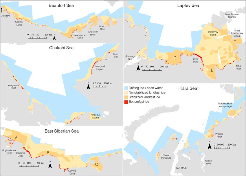
566 D. O. Dammann et al.: Mapping pan-Arctic landfast sea ice stability
Figure 7. (a) Sentinel-1 interferograms derived from image pairs acquired over the Laptev Sea between February and May 2017. Numbers
on images represent date ranges. The colors blue, green, yellow, and red signify the months of February–May. (b, c, d) Three enlarged areas
identified in (a) are further discussed in the text.
The Kara Sea features predominately nonstabilized ice along ities (Fig. 11a) most pronounced near the arch terminus to
the coast and along the outer margins of archipelagos. the south. Near the failure line, there was no sign of a fringe
discontinuity up until 12 April (Fig. 11a), when the interfer-
3.2 Evaluating stability of temporarily stabilized pack ogram displays near-cross-track parallel fringes, indicating
ice compression towards the terminus (Fig. 11b). There is a sig-
nificant contrast in fringe density on either side of the line,
Sentinel-1 SAR backscatter imagery captured the location which may be indicative of a fracture, where the ice to the
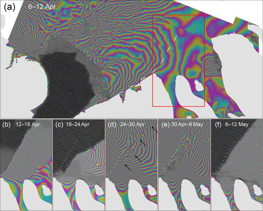
and breakup of the ice arch in Nares Strait in 2017 (Fig. 10). west is being compressed more rapidly than the ice close
This breakup event occurred relatively early compared with to the coast. The interferogram between 18 and 24 April
past events (Kwok, 2005), partly in response to thinner ice features widespread coherence loss, possibly due to contin-
conditions and northerly winds (Moore and McNeil, 2018). ued compression (Fig. 11c). Deformation is less severe from
The arch appeared stable on 6 May (Fig. 10b), before even- 24 April, when the fringe density is significantly reduced.
tually failing sometime before 12 May (Fig. 10c) as seen in However, we did notice a fringe discontinuity to the east of
the SAR backscatter images. The interferograms revealed the the failure line, featuring perpendicular intermediate fringe
ice deformation around the location of fracture up until the patterns following late April (see arrows in Fig. 11d). These
failure event. As seen in the interferograms, the ice arch fea- patterns develop further into circular patterns often associ-
tures various levels of centimeter- to meter-scale deformation ated with vertical lifts and depressions (Fig. 11e), before the
and fractures prior to breakup, resulting in fringe discontinu-
The Cryosphere, 13, 557–577, 2019 www.the-cryosphere.net/13/557/2019/D. O. Dammann et al.: Mapping pan-Arctic landfast sea ice stability 567
Figure 8. (a) Sentinel-1 interferograms derived from image pairs acquired over the Kara Sea between March and May 2017. Numbers on
images represent date ranges. The colors blue, green, yellow, and red signify the months of February–May. (b, c, d) Three enlarged areas
identified in (a) are further discussed in the text.
whole arch appears to fail through shear motion along this are many factors that affect fringe density in addition to sta-
same fault (Fig. 11f). bility, including changing wind and ocean currents, satellite
viewing geometry, and the prevalent mode of ice deforma-
tion (Dammann et al., 2016). A measure of whether ice is
4 Discussion practically stable would also depend on specific stakeholders
and their dependence on stability. For example, on shorter
4.1 Validating stability zones with areas of known ice timescales, industry ice roads would be able to accommo-
stability date less strain than community ice trails, due to differ-
ent modes of transportation and user-specific needs. Further
The InSAR technique used to map bottomfast sea ice was steps to identify such thresholds are outlined in Dammann et
thoroughly validated in several regions by Dammann et al. (2018a).
al. (2018c). The high stability of these regions can be inferred There is limited information that can be used to vali-
from the ice resting on the seafloor. However, other stability date these stability classes – namely, the separation between
zones (i.e., stabilized and nonstabilized ice) are based on rel- stabilized- and nonstabilized ice. Even so, we compared our
ative stability, in terms of whether the ice is anchored or shel- mapping approach here with one region in the Beaufort and
tered. Determining absolute stability (i.e., whether an area is one in the Laptev Sea with areas of known stabilization
stable enough for a specific use, such as ice roads) would be points. We examined a backscatter mosaic from three images
problematic using fringe density alone. This is because there
www.the-cryosphere.net/13/557/2019/ The Cryosphere, 13, 557–577, 2019568 D. O. Dammann et al.: Mapping pan-Arctic landfast sea ice stability Figure 9. InSAR-derived map of nonstabilized and stabilized landfast ice and bottomfast ice from Sentinel-1 image pairs, acquired predom- inantly between March and May 2017. Letters A–G mark areas discussed in the text. Land is masked out in light grey. This map of stability zones is subject to limitations and uncertainties outlined in the text. (8, 15, and 17 April) along the Beaufort Sea coast. These depth of ridges in 2017 or the possibly reduced grounding images exhibit, in certain locations, a sharp discontinuity in strength of ridges present in Node B. Certain sections of the backscatter, which can identify the location of the landfast border between stabilized and nonstabilized ice extend rel- ice edge (see white arrows in Fig. 12a). atively far from the coast (see black arrows in Fig. 12d). The landfast ice edge identified using backscatter is con- At these points, the stability is higher than adjacent areas sistent with the three nodes (A–C) identified by Mahoney et with the same distance from shore. This is consistent with al. (2007, 2014; our Fig. 12b). These nodes signify a per- increased stability behind grounded ridges. sistent landfast ice edge, believed to be a result of reoc- Although the landfast ice edge can in some instances be curring grounded ice features (Mahoney et al., 2014). The mapped using a single backscatter image, stabilized ice can- ice shoreward of these three nodes is expected to be stabi- not easily be discriminated from nonstabilized ice. This is lized, because grounded ridges are known to stabilize land- apparent when comparing grounding locations as obtained fast ice, leading to reduced strain shoreward of the grounding with InSAR with backscatter images (see black arrows in points (Mahoney et al., 2007; Druckenmiller, 2011). Interfer- Fig. 12a). It is also worth noting that relying on backscat- ograms exhibit a phase response, suggesting stabilized ice di- ter to discriminate landfast or drifting ice only works in some rectly shoreward of nodes A and C (Fig. 12c). Here, node A cases. There must be noticeable differences in backscatter be- is known to correspond to the location of large grounded tween landfast and drifting ice, or a severely deformed land- ridges, offering stability to the ice cover (Meyer et al., 2011). fast ice edge as a result of shear interaction with the pack ice Nodes B and C are also expected to be regions of persistent (Druckenmiller et al., 2013). grounded ridges since the nodes coincide roughly with the Similar patterns indicating grounded ridges were found in 20 m isobath (Mahoney et al., 2014). However, ice directly the Laptev Sea, where an April interferogram shows a section shoreward of node B appears nonstabilized, with stabiliza- of stabilized ice roughly 100 km offshore (see A in Fig. 13). tion only further in. This may be due to the reduced keel The full area extent of the stabilized ice cannot be deter- The Cryosphere, 13, 557–577, 2019 www.the-cryosphere.net/13/557/2019/
D. O. Dammann et al.: Mapping pan-Arctic landfast sea ice stability 569
4.2 Methodological limitations for mapping stability
zones
There are a number of sources of uncertainty that affect our
map of landfast ice and its relative stability. Dammann et
al. (2018c) have determined that, in some instances, bottom-
fast ice has to be approximated on the subkilometer scale due
to ambiguities associated with low fringe density or fringes
parallel to the bottomfast ice edge. We also acknowledge that
small islands or sandbars not represented by our landmask
may be erroneously identified as bottomfast ice. We have re-
duced such errors by not mapping areas that appear to be
low-lying land in the SAR backscatter images. However, dis-
criminating between ice and low-lying land can be difficult
based on strictly SAR. Here, other remote-sensing systems
such as optical systems could be applied to further reduce
biases from coastline errors. In areas where the landmask
does not appear to fit the coastline due to errors or coast-
line changes, mapping intricate coastal morphology can be a
time-consuming task – hence mapping on a pan-Arctic scale
will inevitably contain inaccuracies. It is also worth mention-
ing that the other stability zones are mapped against the land-
mask, also likely resulting in errors. However, as the extent of
these zones are larger, the relative contribution of such errors
will be much smaller.
In this work, we did not apply strict mapping thresholds
to distinguish between stabilized and nonstabilized ice but
rather made subjective determinations based on fringe pat-
terns. This approach works well in the Chukchi and Beau-
fort seas, where regions of low fringe density lie adjacent to
the coast or bottomfast ice and can be easily distinguished
from regions of higher fringe density. However, in some re-
gions, especially in the Russian Arctic, there is often a lack of
distinct boundaries between regions of different fringe spac-
Figure 10. Map of Nares Strait (a), and Sentinel-1 backscatter im- ing, introducing ambiguities between stabilized and nonsta-
ages over the 2017 ice arch (blue line in a) before (b) and after (c) bilized ice on scales from kilometers to even tens of kilo-
failure. The line of failure is identified in (c) and marked as a dashed meters (Figs. 6c and 7c). The difficulty of making distinc-
line in (b, c). Land is masked out in light gray. tions between these two zones may result from reduced pack
ice interaction along the Russian shelf, given the predomi-
nately divergent ice regimes (Reimnitz et al., 1994; Alexan-
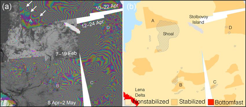
mined due to limited data availability in the region, and one
drov et al., 2000; Jones et al., 2016). This generally results
interferogram had to be acquired as early as February, be-
in reduced ice forcing and landfast ice strain in contrast to
fore this region had stabilized. Stabilized ice is expected in
the western Arctic. These regions are expected to feature re-
this region, which features a large shoal, earlier ice formation
duced dynamically induced strain (and therefore fewer in-
than surrounding areas, and grounded ridges (Selyuzhenok
terferometric fringes) in nonstabilized ice, making it appear
et al., 2015). The location of this large shoal, along with
more stable. This is visible in the different fringe densities
smaller ones, are obtained from Jakobsson et al. (2012) and
of the nonstabilized ice in Figs. 4d and 6d. Additionally, the
displayed in Fig. 13b. Here, it is apparent that even some
greater extent of landfast ice on the shoreward side of the
of the smaller shoals are associated with stabilized ice (see
grounding points provides a greater fetch, which may cause
B and C in Fig. 13b). It is also clear that the extensive stabi-
stabilized ice on the Russian Shelf to exhibit higher fringe
lized ice that stretches out halfway between Great Lakhovsky
densities than in the Chukchi or Beaufort seas. This suggests
Island and Stolbovoy Island is potentially anchored between
that there is likely a spectrum of landfast ice stability. Addi-
the coast and the shallow areas (see D in Fig. 13b).
tional zones may be necessary to fully characterize landfast
ice regimes in different regions for different ice uses or re-
search aims. Expanding on the classes presented here would
www.the-cryosphere.net/13/557/2019/ The Cryosphere, 13, 557–577, 2019570 D. O. Dammann et al.: Mapping pan-Arctic landfast sea ice stability Figure 11. Interferogram over the Nares Strait ice arch in 2017, covering the time period 6–12 April (a). Smaller panels show consecutive interferograms within the box for 12–18 April (b), 18–24 April (c), 24–30 April (d), 30 April–6 May (e), and 6–12 May (f). Dashed line represents the line separating fast and moving ice in Fig. 12c. The black arrows in (d) indicate fringe patterns further discussed in the text. Land is masked out in light gray. likely require a different set of evaluation criteria for fringes, of the Lena Delta, we classified much of the landfast ice in depending on regions. Additional data such as bathymetry this region as nonstabilized (Fig. 9). This suggests the crite- would also likely strengthen this analysis. ria for stabilized ice used in this analysis is different than in We have focused on some examples with possibly subop- Eicken et al. (2005) and can provide new information related timal classification. One potential candidate for reclassifica- to stability in the region. Based on the overall fringe counts tion is landfast ice in sheltered bays, such as the Khatanga and patterns, the majority of the phase response is due to Gulf in the western Laptev Sea, which exhibited predomi- lateral displacement and potentially only partially due to ver- nantly high fringe densities (Fig. 7a). Hence, the Khatanga tical displacement (circular fringe patterns with low density Gulf was largely identified as nonstabilized, despite being – see Dammann et al., 2016) due to tidal motion. It is pos- nearly landlocked (Fig. 9). Due to the shallow water in this sible that landfast ice in this region may be less stable than region, it is likely that the high fringe density is caused previously thought, and that a partially stabilized zone may in part by vertical motion associated with tides and coastal be appropriate. This would be consistent with a recent SAR setup. Since vertical motion has less impact on stability in backscatter analysis of landfast ice in the Laptev Sea (Se- well-confined landfast ice, such examples suggest the poten- lyuzhenok et al., 2017), which showed that areas identified tial need for an additional zone of stability, allowing higher as landfast ice in operational ice charts may actually contain fringe densities in coastally confined regions. Such additional pockets of partly mobile ice. This was shown for the month classification would depend on other data sets such as a land- after initial landfast ice formation, but could possibly result mask or bathymetry to identify the level of restricted ice in more dynamic ice throughout spring due to reduced ice movement in response to likely forcing conditions. Another, thickness. larger-scale example is the eastern Laptev sea, which is an Sensitivity to specific atmospheric and oceanographic con- area of landfast ice sheltered by the New Siberian Islands and ditions during the time period between SAR acquisitions is typically considered stable (Eicken et al., 2005). However, may place a limitation on the number of stability zones that based on relatively high fringe density, particularly offshore can be mapped. For example, in the absence of dynamic The Cryosphere, 13, 557–577, 2019 www.the-cryosphere.net/13/557/2019/
D. O. Dammann et al.: Mapping pan-Arctic landfast sea ice stability                                                                     571

Figure 12. (a) Sentinel-1 backscatter images over the western Beaufort Sea. White arrows signify the landfast ice edge as identified by
contrasting backscatter. (b) Landfast ice edge occurrence mapped for the period 1996–2008 over the Alaska Beaufort Sea (Mahoney et
al., 2014). Light red circles correspond to areas of frequent landfast ice edge formation, referred to as “nodes”. (c) Interferograms between
mid-April and mid-May 2017. (d) Different stability zones derived from (c). Potential grounding points as identified in (d) are marked with
black arrows in (d, a). Land is masked out in light gray.

interaction with pack ice, there may be little difference in             bility as possible (roughly late April), but once had to be ob-
fringe spacing between landfast ice seaward and shoreward                tained as early as February. Fringe density tends to decrease
of stabilizing anchor points. Without evaluating the phase re-           over the winter as the ice thickens (Dammann et al., 2016).
sponse for each area of interest in detail during different forc-        Hence, the use of interferograms based on different dates can
ing scenarios, it may be difficult to understand under what              aid interpretation by confirming consistent fringe patterns
conditions the ice remains stable. Classification of stability           and discontinuities that identify temporal changes. Temporal
based on relative differences in fringe density is also compli-          changes result in phase discontinuities at the image stitchings
cated by the use of nonsimultaneous interferograms to pro-               that are not related to different stability zones, which further
vide complete coverage of a region. The interferograms used              complicates the mapping process.
here were obtained as close to maximum ice extent and sta-

www.the-cryosphere.net/13/557/2019/                                                                The Cryosphere, 13, 557–577, 2019
572                                                         D. O. Dammann et al.: Mapping pan-Arctic landfast sea ice stability

Figure 13. (a) Sentinel-1 interferograms over Laptev Sea near Stolbovoy Island between February and May 2017. (b) Outlined nonstabilized
(light orange) and stabilized (dark orange) ice. Shallow areas (< 10 m; Jakobsson et al., 2012) are marked with gray cross hatching. Stabilized
ice that is likely supported by grounding near shallow features are marked A–D and further discussed in the text. Land is masked out in light
gray.

   Sentinel-1 IW imagery is predominantly acquired over                   for both long-term strategic planning and short-term tactical
land, so it is likely not possible to construct interferograms            decisions. Using interferograms generated by a standardized
away from the coast, for extensive landfast ice approaching               workflow, we show that three stability zones of landfast ice
the 250 km IW swath, such as that in the East Siberian Sea.               can be identified based on fringe density and continuity, in-
Data availability further restricts the temporal baseline be-             dicative of differential ice motion occurring between SAR
tween images to a minimum of 12 days, though this now rep-                acquisitions. Along the Beaufort Sea coast of Alaska, we find
resents a shorter period than past work identifying landfast              that the landfast ice regime can be well described with three
ice (Mahoney et al., 2004; Meyer et al., 2011; Dammann et                 stability zones: bottomfast ice, where the sea ice is frozen to
al., 2016). Further studies should investigate the effect of dif-         or resting on the seabed; stabilized ice, which is floating but
ferent temporal baselines on the stability product. A shorter             sheltered by coastlines or anchored by islands or grounded
baseline will result in higher temporal resolution. However,              ridges; and nonstabilized ice, which represent floating exten-
with a shorter baseline (e.g., Sentinel-1 6-day baseline), map-           sions seaward of any anchoring points. These findings are
ping of the seaward landfast ice edge may incorporate sta-                supported by comparison with the location of stable nodes,
tionary pack ice. A longer baseline will result in lower inter-           identified through analysis of hundreds of landfast ice edge
ferometric coherence. With a 12-day baseline, some regions,               positions over the period 1996–2008. Not only does this pro-
such as the Kotzebue Sound region, already feature consis-                vide some validation of our results, but it demonstrates the
tent coherence loss. Such regions can most often be identified            ability of InSAR to capture useful information in just two
through a spatially inconsistent progression, from high to a              snapshots, compared to previously requiring analysis over
complete loss of coherence. In such cases, the mapping of                 many years.
landfast ice type boundaries is not possible. It is worth men-               Based on our findings, it is likely that InSAR-derived maps
tioning that this technique can only be used before the onset             could provide substantial value as a standalone product for
of melt, when widespread coherence loss occurs. Therefore,                some regions such as the Beaufort Sea. With that said, the
it is not possible to evaluate the retreat of bottomfast ice or           stability zones in the Beaufort Sea and the Russian Arctic ap-
the reduction of ice stability in response to melt.                       pear to be qualitatively different. This makes it challenging to
                                                                          directly adapt the proposed scheme to the East Siberian and
                                                                          Laptev seas, which are associated with substantial uncertain-
5   Conclusion                                                            ties. Even so, we demonstrate the data availability and ap-
                                                                          plication of this InSAR-based approach, which can provide
In a time of rapidly changing sea ice conditions and contin-              added value to ice charts and other products. In ice chart-
ued interest in the Arctic from a range of stakeholders, we               ing, multiple information products are evaluated with local
stress the need for new assessment strategies to enable safe              knowledge to create final products. Similarly, the value of In-
and efficient use of sea ice. InSAR is gaining growing atten-             SAR may be greatly enhanced by linking it with other prod-
tion in the sea ice scientific community, and here we demon-              ucts (e.g., InSAR time series analysis, SAR-based and opti-
strate its value for identifying zones of landfast ice stabil-            cal remote-sensing products, local knowledge, coastal mor-
ity. We are also highlighting the application of InSAR for                phology and bathymetry, and atmospheric and ocean forcing
the development of operational sea ice information products,              data).

The Cryosphere, 13, 557–577, 2019                                                                www.the-cryosphere.net/13/557/2019/
You can also read


