Spatial distribution of cloud droplet size properties from Airborne Hyper-Angular Rainbow Polarimeter (AirHARP) measurements
←
→
Page content transcription
If your browser does not render page correctly, please read the page content below
Atmos. Meas. Tech., 13, 1777–1796, 2020
https://doi.org/10.5194/amt-13-1777-2020
© Author(s) 2020. This work is distributed under
the Creative Commons Attribution 4.0 License.

Spatial distribution of cloud droplet size properties from Airborne
Hyper-Angular Rainbow Polarimeter (AirHARP) measurements
Brent A. McBride1,2,3 , J. Vanderlei Martins1,2,3 , Henrique M. J. Barbosa4 , William Birmingham2,3 , and
Lorraine A. Remer2,3
1 Department   of Physics, University of Maryland Baltimore County, Baltimore, Maryland, USA
2 Earth  and Space Institute, University of Maryland Baltimore County, Baltimore, Maryland, USA
3 Joint Center for Earth Systems Technology, University of Maryland Baltimore County, Baltimore, Maryland, USA
4 Instituto de Física, Universidade de São Paulo, São Paulo, 05508-090, Brazil

Correspondence: Brent A. McBride (mcbride1@umbc.edu)

Received: 7 October 2019 – Discussion started: 23 October 2019
Revised: 11 February 2020 – Accepted: 17 February 2020 – Published: 8 April 2020

Abstract. The global variability of clouds and their inter-        are made for cloud fields that stretch both across the swath
actions with aerosol and radiation make them one of our            and along the entirety of a flight observation. During the
largest sources of uncertainty related to global radiative forc-   NASA Lake Michigan Ozone Study (LMOS) aircraft cam-
ing. The droplet size distribution (DSD) of clouds is an ex-       paign in May–June 2017, the Airborne HARP (AirHARP)
cellent proxy that connects cloud microphysical properties         instrument observed a heterogeneous stratocumulus cloud
with radiative impacts on our climate. However, traditional        field along the solar principal plane. Our retrievals from this
radiometric instruments are information-limited in their DSD       dataset show that cloud DSD heterogeneity can occur at the
retrievals. Radiometric sensors can infer droplet effective ra-    200 m scale, much smaller than the 1–2 km resolution of
dius directly but not the distribution width, which is an im-      most spaceborne sensors. This heterogeneity at the sub-pixel
portant parameter tied to the growth of a cloud field and to       level can create artificial broadening of the DSD in retrievals
the onset of precipitation. DSD heterogeneity hidden inside        made at resolutions on the order of 0.5 to 1 km. This study,
large pixels, a lack of angular information, and the absence of    which uses the AirHARP instrument and its data as a proxy
polarization limit the amount of information these retrievals      for upcoming HARP CubeSat and HARP2 spaceborne in-
can provide. Next-generation instruments that can measure          struments, demonstrates the viability of the HARP concept
at narrow resolutions with multiple view angles on the same        to make cloud measurements at scales of individual clouds,
pixel, a broad swath, and sensitivity to the intensity and po-     with global coverage, and in a low-cost, compact CubeSat-
larization of light are best situated to retrieve DSDs at the      sized payload.
pixel level and over a wide spatial field. The Airborne Hyper-
Angular Rainbow Polarimeter (HARP) is a wide-field-of-
view imaging polarimeter instrument designed by the Uni-
versity of Maryland, Baltimore County (UMBC), for re-              1   Introduction
trievals of cloud droplet size distribution properties over a
wide swath, at narrow resolution, and at up to 60 unique, co-      Clouds are one of the most uncertain aspects of our climate
located view zenith angles in the 670 nm channel. The cloud        system. Clouds are highly variable, yet well-dispersed across
droplet effective radius (CDR) and variance (CDV) of a uni-        the globe and play a dual role in distributing energy: they
modal gamma size distribution are inferred simultaneously          trap infrared radiation in our atmosphere and reflect short-
by matching measurement to Mie polarized phase functions.          wave radiation back to space (Rossow and Zhang, 1995).
For all targets with appropriate geometry, a retrieval is pos-     This energy distribution is the key unknown in predicting cli-
sible, and unprecedented spatial maps of CDR and CDV               mate change, as the interplay between longwave trapping and
                                                                   shortwave reflection of radiation by clouds may change sig-

Published by Copernicus Publications on behalf of the European Geosciences Union.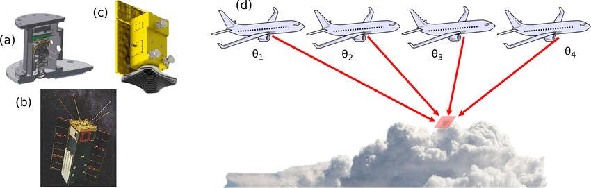
1778            B. A. McBride et al.: Spatial distribution of cloud droplet size properties from AirHARP measurements

nificantly as the planet warms. The relative strength of these     lite instruments allow us to make these long-term connec-
impacts depends strongly on cloud macrophysical and mi-            tions between radiation and the evolution of cloud DSDs for
crophysical properties, such as cloud optical thickness, ther-     different cloud types and over large spatial and temporal pe-
modynamic phase, cloud-top temperature, height, and pres-          riods. Also, satellite studies best improve global models that
sure, liquid and ice water path and content, and droplet size      examine both future climate scenarios and cloud feedbacks
distributions. Measuring these elements in a global context        (Stubenrauch et al., 2013).
and over long temporal scales is crucial to improving our un-         There are currently two methods used to retrieve CDR
derstanding of how cloud properties translate to a radiative       from spaceborne instruments. The first is the widely used
impact on climate.                                                 radiometric bi-spectral retrieval, first proposed by Naka-
   Clouds also share a delicate relationship with aerosols.        jima and King (1990) and employed operationally to the
Aerosols drop the energy barrier required for condensation,        MODerate resolution Imaging Spectroradiometer (MODIS)
serving as condensation nuclei (Petters and Kreidenweis,           and other multi-band radiometer data (Platnick et al., 2003,
2007) for liquid water and ice clouds in our atmosphere.           2017; Walther and Heidinger, 2012). The bi-spectral retrieval
When aerosols are entrained into a cloud, they can set off         uses the difference in cloud information content observed by
a condensation feedback loop, but in some cases, the oppo-         shortwave infrared (i.e., 1.6, 2.1, or 3.7 µm) and visible (i.e.,
site occurs: they dry out the local atmosphere and evapo-          0.67 or 0.87 µm) channels to retrieve CDR and cloud optical
rate smaller droplets (Hill et al., 2009; Small et al., 2009).     thickness (COT) simultaneously for a cloud target. The sec-
Aerosols can invigorate convective clouds (Altaratz et al.,        ond method is the multi-angle polarimetric retrieval, which
2014) and suppress the development of other clouds (Koren          is relatively new. The polarimetric retrieval corresponds to a
et al., 2004), depending on the aerosol and meteorological         parametric fit to a multi-angle polarized cloudbow (or rain-
properties of the local atmosphere. This complexity is a ma-       bow by cloud droplets) structure that is sensitive to both CDR
jor source of uncertainty related to understanding global ra-      and CDV simultaneously (Breon and Goloub, 1998; Alexan-
diative forcing and predicting climate change (Boucher et al.,     drov et al., 2015; Di Noia et al., 2019). COT can also be
2013; Rosenfeld et al., 2014; Penner et al., 2004; Coddington      retrieved with assistance from an external radiative trans-
et al., 2010).                                                     fer simulation (Alexandrov et al., 2012a). The 3D multiple
   A major link between the radiative and microphysical cli-       scattering effects of shadowing and illumination (Marshak
mate impacts of liquid water clouds is the droplet size distri-    et al., 2006; Varnai and Marshak, 2002) bias the radiomet-
bution (DSD). A common mathematical representation of the          ric method, whereas the polarimetric retrieval is sensitive
liquid water cloud DSD is a gamma distribution (Tampieri           to scattered photons from a COT up to ∼ 3, lessening the
and Tomasi, 1976; Hansen, 1971; Alexandrov et al., 2015).          impact of this effect (Miller et al., 2018). Sub-pixel clouds
This DSD is formed by two parameters, cloud droplet effec-         and spatial heterogeneities can affect both methods, as dis-
tive radius (CDR or reff ) and effective variance (CDV or veff ;   cussed in later sections (Zhang and Platnick, 2011; Breon and
Hansen and Travis, 1974), which represent the mean droplet         Doutriaux-Boucher, 2005; Shang et al., 2015). Furthermore,
size and dispersion relative to the scattering cross section.      the bi-spectral technique is not sensitive to CDV and uses a
Aerosol effects on cloud microphysics are strongly tied to         preestablished value (0.1, Platnick et al., 2017) that may not
the CDR (Twomey, 1977; Albrecht, 1989). In a general ex-           be valid for all liquid water cloud targets and all regions of
ample, aerosol loading generates competition for condensa-         the world.
tion sites and leads to smaller droplets. This process can de-        Multi-angle polarimetric measurements have other advan-
lay rainout but increase the overall liquid water content, ex-     tages for cloud characterization beyond the retrieval of the
tending the lifetime of the cloud. An abundance of smaller         two DSD parameters. We find that retrievals of cloud thermo-
droplets scatters shortwave radiation efficiently, creating a      dynamic phase (Riedi et al., 2010; Goloub et al., 2000), ice
brighter cloud, and finally the excess of radiation to space       crystal asymmetry (van Diedenhoven et al., 2013), aerosol
results in a net cooling of the planet (Haywood and Boucher,       above cloud (Waquet et al., 2013), and COT (Xu et al., 2018;
2000; Lohmann et al., 2000, and references therein). Typ-          Cornet et al., 2018) are considerably improved with the ad-
ically, studies that connect the microphysical and radiative       dition of polarized observations. At the time of this writing,
properties of clouds do so by tracking changes in CDR only,        only the Polarization and Directionality of the Earth’s Re-
with no direct sensitivity to CDV (Feingold et al., 2001; Plat-    flectances (POLDER; Deschamps et al., 1994) instruments
nick and Oreopoulos, 2008). Because CDV is a measure-              have demonstrated the polarized retrieval of cloud DSD
ment of the breadth of the DSD, it may encode information          properties from space, though several aircraft instruments,
on cloud growth processes: collision–coalescence, aerosol or       including the Airborne Multi-angle SpectroPolarimetric Im-
dry air entrainment, evaporation, and the initiation of precip-    ager (AirMSPI; Diner et al., 2013), the Research Scanning
itation on cloud cores or peripheries. Not all clouds share the    Polarimeter (RSP; Cairns et al., 1999), and the subject of
same relationship between microphysics and radiation, but          this paper, the Airborne Hyper-Angular Rainbow Polarime-
the key to understanding the connection lies in the micro-         ter (AirHARP; Martins et al., 2018), have demonstrated im-
physics described by these two DSD parameters. Only satel-

Atmos. Meas. Tech., 13, 1777–1796, 2020                                              www.atmos-meas-tech.net/13/1777/2020/
B. A. McBride et al.: Spatial distribution of cloud droplet size properties from AirHARP measurements                             1779

                                                                        tions. Instruments like POLDER, which samples at 14 unique
                                                                        viewing angles separated by 10◦ , do not provide enough na-
                                                                        tive angular resolution (Shang et al., 2015) and, as a conse-
                                                                        quence, may not be able to identify wide versus narrow DSD
                                                                        clouds at specific geometries (Miller et al., 2018). Only when
                                                                        sampling all native 6×7 km POLDER pixels inside a 150 km
                                                                        superpixel can they access the full scattering angle cover-
                                                                        age in Fig. 1 and perform an accurate retrieval (Breon and
                                                                        Goloub, 1998). However, this limits their retrievals to large-
                                                                        scale, homogenous marine stratocumulus clouds with narrow
                                                                        DSDs. In a study by Breon and Doutriaux-Boucher (2005), a
                                                                        comparison between POLDER polarized and MODIS radio-
                                                                        metric retrievals showed a CDR bias of 2 µm that could not
                                                                        be fully decoupled from the large POLDER superpixel. Later
                                                                        evaluation by Alexandrov et al. (2015), with the RSP and
                                                                        the Autonomous Modular Sensor spectrometer, found that
                                                                        the CDR values retrieved by the two methods agree at nar-
                                                                        rower resolution. Shang et al. (2015) improved the POLDER
                                                                        retrieval by reducing the superpixel to 42 km. Even though
                                                                        sampling at higher resolution produced gaps in cloudbow
                                                                        coverage, they still found heterogeneity inside the original
                                                                        150 km superpixel using this improved method. In a follow-
                                                                        up paper, Shang et al. (2019) showed that the POLDER re-
                                                                        trieval is sensitive to a wider CDR and CDV range and can
                                                                        be done at a lower 40–60 km resolution when considering all
                                                                        three polarized wavelengths (490, 670, and 865 nm) in the
                                                                        retrieval. Even so, no instrument thus far has performed a
                                                                        polarimetric cloud retrieval from space with both co-located
                                                                        pixel resolution less than 40 km and high native angular den-
                                                                        sity (< 10◦ ). These goals are essential to studying the spatial
Figure 1. Mie scattering simulations for liquid water cloud droplets,
with solar light incident, for the four HARP wavelengths at 10 µm
                                                                        distribution of DSDs for heterogeneous, broken, and popcorn
CDR and 0.02 CDV (a), the 0.67 µm channel for variable CDR and          cumulus cloud scenes other than the conventional retrievals
constant CDV (b), and constant CDR with variable CDV (c).               from marine stratocumulus cases.
                                                                           The benefit of aircraft instruments like RSP, AirMSPI, and
                                                                        AirHARP is to demonstrate new technologies that improve
                                                                        upon the POLDER retrieval heritage. RSP, in particular, sam-
proved sampling schemes, resolution, and accuracy (Knobel-              ples at 150+ viewing angles, separated on average by ∼ 0.8◦ ,
spiesse et al., 2019; van Harten et al., 2018).                         and does so for a co-located 250 m along-track pixel (Alexan-
   Not all polarimetric measurements will achieve a high-               drov et al., 2012b, 2015, 2016b). This advancement removes
quality retrieval of cloud DSDs. Multi-angle sampling at high           any large-scale homogeneity assumptions and allows for a
angular density and moderate pixel resolution is an essen-              rainbow Fourier transform on the data, one that retrieves the
tial element of an accurate single-wavelength retrieval. Fig-           DSD itself, including multiple modes, without any assump-
ure 1 shows theoretical Mie simulations that mimic the polar-           tions on the distribution shape (Alexandrov et al., 2012b).
ized cloudbow for particular values of CDR, CDV, and wave-              RSP can sample other kinds of clouds, including broken and
length. To resolve the cloudbow patterns from space and re-             popcorn cumulus clouds, with high angular and spatial reso-
trieve the CDR and CDV of the cloud, the multi-angle po-                lution and does so with high polarimetric accuracy (Cairns et
larimetric instruments must satisfy a minimum viewing an-               al., 1999). The single-pixel cross-track swath of RSP, how-
gle density (Miller et al., 2018), which is directly related to         ever, restricts its spatial coverage: RSP cannot form an in-
scattering angle coverage. The location of the supernumer-              tuitive image of the scene, requires specific solar angles for
ary peaks in scattering angle encode CDR in the 0.67 µm ex-             cloudbow coverage (Alexandrov et al., 2012b), and requires
ample shown in Fig. 1. To resolve the CDV, the amplitude of             input from other coincident instruments for off-nadir con-
the supernumerary peaks must be detected. Polarimeters with             text (Alexandrov et al., 2016a). Conversely, the AirMSPI in-
coarser viewing angle separation for a single wavelength                strument is a highly accurate push-broom imager capable of
(i.e., > 3◦ at 0.67 µm for typical droplets < 15 µm; Miller             discrete, programmable viewing angles on the same target,
et al., 2018) may not distinguish these cloudbow oscilla-               but it has the same angular limitations as POLDER in this

www.atmos-meas-tech.net/13/1777/2020/                                                     Atmos. Meas. Tech., 13, 1777–1796, 2020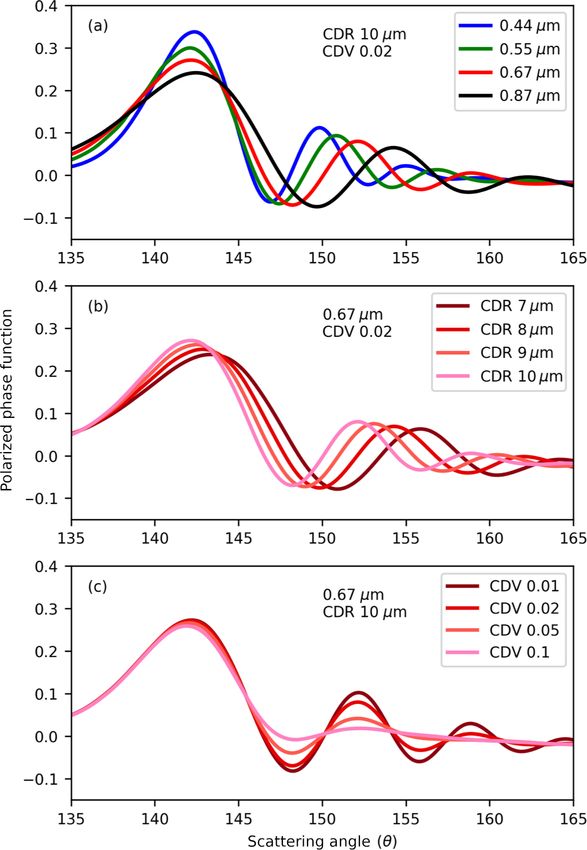
1780            B. A. McBride et al.: Spatial distribution of cloud droplet size properties from AirHARP measurements

step-and-stare mode. AirMSPI also samples in a continuous           is split by a Phillips prism toward three detectors. Before
sweep mode that trades co-located information for scattering        reaching each detector, this light passes through a polarizer
angle coverage (Diner et al., 2013). This mode gives full vi-       oriented at 0, 45, or 90◦ . The polarizers are oriented at 45◦
sual coverage on the cloudbow but limits the retrieval to a line    separations such that the I , Q, and U Stokes parameters of
cut of binned pixels along the solar principal plane. A study       the scene can be retrieved in a single co-aligned pixel from an
by Xu et al. (2018) extended the AirMSPI line-cut retrieval to      orthogonal basis set of polarization states (Fernandez-Borda
the entire continuous sweep image of the cloudbow with as-          et al., 2009). AirHARP images a ground scene with a ±57◦
sistance from image-specific empirical correlations between         (±47◦ ) along-track (cross-track) FOV, and a custom stripe
COT, CDR, and CDV. This line-cut polarimetric technique             filter over the detector assigns 120 along-track portions, or
requires a droplet size homogeneity assumption over the full        view sectors, of the FOV to four visible channels (band-
line cut of the cloudbow, which may blur heterogeneity that         widths): 440 (14), 550 (12), 670 (18), and 870 (37) nm. A
exists at the pixel level and steer the retrieval towards wider     view sector specifically defines a segment of the detector that
DSDs.                                                               corresponds to a unique average viewing angle at the front
   There is a strong interest in the Earth science community        lens. The hyper-angular 670 nm band samples at 60 view sec-
in a multi-angle polarimeter concept for aerosol and cloud re-      tors at an average 2◦ separation, and the other three channels
trievals with a wide swath for spatial context, high accuracy       sample at 20 each at an average 6◦ separation. In this way,
in polarization, high angular density for cloudbow retrieval,       the 60 670 nm view sectors can sample the cloudbow oscilla-
and narrow ground resolution (Remer et al., 2019; Dubovik           tions at high angular density without large-scale homogene-
et al., 2019). The Earth and Space Institute (ESI) at the Uni-      ity assumptions or degrading the measurement for scattering
versity of Maryland, Baltimore County (UMBC), designed,             angle coverage. The wide FOV also allows for broad scat-
developed, and deployed the Airborne Hyper-Angular Rain-            tering angle coverage from space during the daylit portion
bow Polarimeter (AirHARP), a next-generation wide-field-            of an orbit. The 20 view sectors in the other three chan-
of-view (FOV) imaging polarimeter specifically for this pur-        nels ensure multi-angle coverage on aerosols; several studies
pose. AirHARP is the aircraft demonstration of spaceborne           show that fewer than seven unique views in a single channel
technology that will fly on a stand-alone CubeSat platform          are appropriate for high-accuracy retrieval of aerosol optical
in 2019 in the orbit of the International Space Station and an      properties (Hasekamp and Landgraf, 2007; Hasekamp et al.,
enhanced HARP sensor for the NASA Plankton–Aerosol–                 2019), though the details are beyond the scope of this paper.
Cloud–ocean Ecosystem (PACE) mission, called HARP2, in              AirHARP is a push-broom imager, meaning that consecutive
the early 2020s.                                                    measurements from a single view sector can be stitched to-
   In this paper, we will first describe the HARP concept and       gether to form an image of a ground scene as observed only
frame the AirHARP instrument and its data as a proxy for            from that angle. These push brooms can have any along-track
upcoming HARP CubeSat and HARP2 space instruments                   length but a cross-track swath proportional to the flight al-
throughout the rest of the work. We then explain the cloud          titude multiplied by a factor of 2.14. This factor accounts
droplet retrieval framework in Sect. 3, followed by applica-        for the maximum AirHARP cross-track view angle, ±47◦ . A
tions of the retrieval on a stratocumulus cloud deck observed       unique push broom is made for each of the 120 view sectors,
by AirHARP during the NASA Lake Michigan Ozone Study                and post-processing registers all of them to a common grid.
field campaign in 2017 in Sect. 4. In Sect. 5, we make use              A target, either on the ground or in the atmosphere, will
of the fine spatial resolution of the retrieved DSD parameters      be viewed from a subset of the 120 view sectors with its re-
to explore the information content of the retrieval itself and      flected apparent I , Q, and U measured in each view sector
relate the spatial variability of the results to cloud processes.   and wavelength. From these measurements, the polarized re-
Section 6 discusses the uncertainties and current limitations       flectance as a function of scattering angle can be compared
of the procedure, and we conclude the paper in Sect. 7, look-       with theoretical Mie calculations, as in Fig. 1. The hyper-
ing ahead to HARP CubeSat and HARP2 deployment and                  angular capability of the 670 nm channel with its 2◦ viewing
data content.                                                       angle resolution can best measure the supernumerary loca-
                                                                    tion and amplitude of the cloudbow structure and is therefore
                                                                    best for retrieving the CDR and CDV of the target cloud.
2   Airborne Hyper-Angular Rainbow Polarimeter                      Note that because AirHARP is an imager, each pixel in the
                                                                    image is a potential target viewed by multiple angles. There-
The AirHARP concept, and the HARP family of polarime-               fore, each pixel in the image can produce its own polar-
ters in general, was developed with a wide swath, fine angular      ized reflectance and can be used to retrieve CDR and CDV,
resolution, and high polarization accuracy to address some          granted that the range of view angles spans a sufficient range
of the limitations of modern polarimeters. The three HARP           of scattering angles. Note that the scattering angle range is
instruments, shown in Fig. 2, are amplitude-splitting, wide-        dependent on both the view angle range (fixed by the instru-
FOV polarimetric cameras. Incident light enters through the         ment) and solar geometry (not fixed). If a large number of
wide-FOV front lens, passes through telecentric optics, and         pixels in the image are viewed at the correct geometry then a

Atmos. Meas. Tech., 13, 1777–1796, 2020                                               www.atmos-meas-tech.net/13/1777/2020/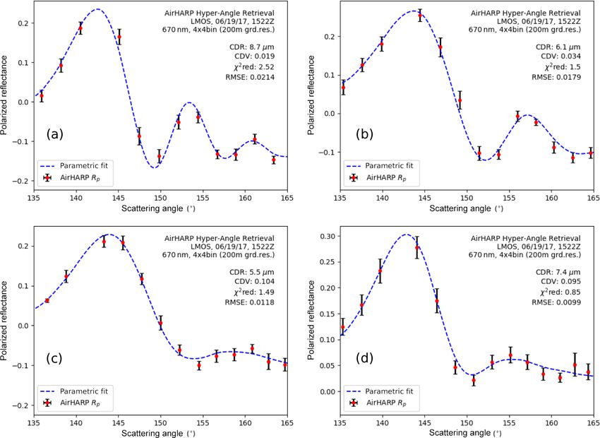
B. A. McBride et al.: Spatial distribution of cloud droplet size properties from AirHARP measurements 1781
Figure 2. Panels (a), (b), and (c) illustrate the current HARP VNIR polarimeter family consisting of the AirHARP airborne system (a),
HARP CubeSat (b), and HARP2 for the NASA PACE mission (c). The HARP concept comprises a wide-field-of-view imaging polarimeter
that images the same ground target from up to 60 distinct viewing angles at 0.67 µm (d) and up to 20 viewing angles at 440, 550, and 870 nm.
The wide cross-track swath (94◦ ) of HARP2 allows for global coverage from space within 2 d.
spatial map can be made of the DSD parameters across and 3 Retrieval framework
along the swath, wherever a cloud pixel is found. Depend-
ing on the observation altitude and binning scheme, ∼ 0.2 to A simple treatment of the parametric retrieval is described
6 km native retrieval resolutions are possible. Therefore, the below, with main components derived from Breon and
microphysics of individual fair-weather cumulus clouds can Goloub (1998), Alexandrov et al. (2015), and Diner et
be retrieved across a cloud field stretching tens to hundreds of al. (2013). The interaction between incident light and a liquid
kilometers. This capability is unprecedented for any existing water cloud droplet is described by a scattering matrix:
multi-angle polarimeter instrument.
In HARP’s current configuration, all of this retrieval po- I P11 P12 0 I
σsca
tential fits entirely inside a 10 × 10 × 15 cm enclosure. The
Q = P12 P22 0 Q , (1)
U 4π R 2 0 0 P U
flagship version of HARP is a spaceborne CubeSat, a stand- sca 33 inc
alone payload funded by NASA’s Earth Science Technology
Office (ESTO) In-space Validation of Earth Science Tech- where a Stokes column vector describes the incident beam
nologies (InVEST) and in collaboration with the Space Dy- (subscript “inc”), in total radiance (I ) and polarized radiance
namics Laboratory (SDL) in Logan, Utah, USA. The HARP (Q, U ), and the scattered beam by a similar vector with sub-
CubeSat satellite was launched on 2 November 2019 to the script “sca”. In general, 16 elements describe the scattering
International Space Station (ISS) (400 km, 51.6◦ inclined or- matrix, but since circular polarization in the atmosphere is
bit) and then dispatched from the station for an autonomous negligible (Cronin and Marshall, 2011) and not measured by
year-long mission in February 2020. Cloud retrievals on AirHARP, the fourth column and row are neglected. Cloud-
HARP CubeSat data will be possible at a minimum 4 km top liquid water droplets are spherical, randomly oriented,
superpixel, a capability demonstrated in this paper using and mirror symmetric: any matrix elements in Eq. (1) that de-
AirHARP, a near-identical copy of the CubeSat instrument scribe asymmetry are neglected and the others mirror across
for aircraft. A third HARP concept, HARP2, is currently un- the main diagonal (Hansen and Travis, 1974). The unitless
der development for the PACE mission to launch in the early Pmn matrix elements scale by the droplet scattering cross sec-
2020s. The HARP CubeSat will be the first satellite to per- tion (σsca ) weighted by the inverse of droplet surface area.
form wide-swath polarized cloud retrievals at sub-5 km co- Sunlight incident on the atmosphere is unpolarized
located resolution from space, and HARP2 will continue this (Qinc , Uinc = 0). For single-scattered photons, the scattered
capability forward and expand it to provide global coverage intensity (Isca ) is proportional to the first matrix element,
in 2 d. P11 and its polarization (Qsca ) to the second, P12 , called the
The remainder of this paper will discuss the information polarized phase function. Usca does not contain any struc-
content retrieved from complex cloud scenes observed by tural information in the scattering plane, though it may show
AirHARP. The study below refers specifically to AirHARP a weak linear slope in the presence of non-cloud scatterers
datasets, but the HARP term may be used when discussing (Alexandrov et al., 2012a). For this reason, Qsca in the scat-
general performance expected from any of the HARP instru- tering plane represents the entire polarized signal.
ments. At the top of the atmosphere (TOA), remote sensors do not
observe the scattering from individual droplets but the bulk
www.atmos-meas-tech.net/13/1777/2020/ Atmos. Meas. Tech., 13, 1777–1796, 2020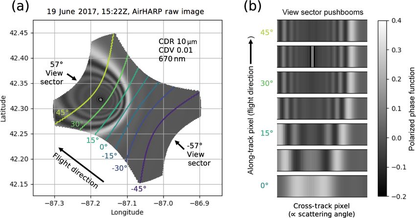
1782            B. A. McBride et al.: Spatial distribution of cloud droplet size properties from AirHARP measurements

behavior of the droplet distributions due to measurement res-          A prescribed lookup table (LUT) in CDR and CDV drives
olution and scale limitations. The bulk Mie polarized phase         the parametric fit, ranging between 5 and 20 µm in CDR
function, hP12 i, is a weighed sum of optical properties:           (1 = 0.5 µm), and CDV values of 0.004 to 0.3 at variable in-
                                                                    tervals, similar to Alexandrov et al. (2015), with 1 values in-
hP12 (λ, θ, CDR, CDV)i                                              dicating the step size. The LUT is dense for CDV < 0.1: the
                                                                    majority of supernumerary bow sensitivity exists below this
    P
       P12,i (λ, θ, CDR, CDV) ωi (λ) Cext,i (λ)
 =
     i
                 P                              ,            (2)    level and is considerably reduced for CDV > 0.1, as shown
                    ωi (λ) Cext,i (λ)                               in Fig. 1. Polarized reflectance measurements are corrected
                  i                                                 via Eq. (3) and fit in a nonlinear least-squares process to
where ω is the single-scattering albedo (SSA, 1 for water           Eq. (4), checking all possible combinations of CDR and CDV
droplets), and Cext is the scattering cross section, which itself   in the LUT. The root mean square error (RMSE) and reduced
                                                                                           2 of the least-squares process verify all
                                                                    chi-square statistic χred
is composed of the scattering efficiency and a size distribu-
tion weighted by droplet cross section. This study uses the         LUT comparisons:
same unimodal gamma size distribution function as Breon                        r
                                                                                 1 Xn                   2
and Goloub (1998). Polarized reflectance observed at TOA            RMSE =             i
                                                                                         Rfit,i − Robs,i ,                      (5)
from liquid water cloud droplets is proportional to P12 , after                  n
a correction for viewing geometry:                                  and
                                                                              1 Xn (Rfit,i − Robs,i )2

         4              −π Qsca                                      2
Robs = (µ0 + µ)                    ,                          (3)   χred =                             .                          (6)
        π                µ0 F0                                               n−5 i       σobs,i 2

where the cosines of the view zenith angle (µ0 ) and so-            The χred 2 verifies that the data are best described by the fit

lar zenith angle (µ) and the band-weighted extraterrestrial         in Eq. (4) with n − 5 degrees of freedom (for three fit pa-
solar irradiance (F0 ) rescale the polarized radiance (Qsca ).      rameters, CDR, and CDV), where n is the number of mea-
The bracketed term is the polarized reflectance (ρP ), and a        surements in the cloudbow scattering angle range for that
similar expression gives the total reflectance (ρ) using the        pixel. Like Alexandrov et al. (2015), a fine-scale interpola-
Stokes parameter Isca in place of −Qsca . Subsequent fig-           tion is performed on the LUT at 10 times the original resolu-
ures use L670 nm for Isca and LP,670 nm for Qsca radiances,         tion in CDR and CDV. Retrievals are accepted immediately
where applicable, and anytime the term intensity is used,           for χred2 values 0.5 to 1.5. In this range, our error estimate

it corresponds to a radiance measurement, not reflectance,                                                          2 is outside this
                                                                    is consistent with the minimized fit. If the χred
unless explicitly noted. Because we are only using a single                                                     2 < 0.5) or underfit
                                                                    range, our error may lead to an overfit (χred
wavelength in our retrieval, radiance and reflectance are in-           2 > 1.5). However, large χ 2 does not always mean the
                                                                    (χred                               red
terchangeable in terms of the information content shown in          fit is poor in our case: the physics of the cloud field may jus-
the figures. Corrections to Eq. (3) for Rayleigh scattering         tify solutions with χred 2 beyond 1.5. Therefore, we also check

at observation height are performed in prior studies (Breon         to see if the fit satisfies an RMSE threshold of 0.03. If not, the
and Goloub, 1998; Diner et al., 2013), but the necessity is         fit is rejected and the pixel is flagged. These diagnostics were
disputed (Alexandrov et al., 2015): this study accounts for         found by a sensitivity study on synthetic AirHARP cloudbow
Rayleigh effects in a weak cosine term described below.             retrievals and an estimation of the error in the actual data.
   The retrieval compares Eq. (3) to a parametric model and             There are several reasons for this two-factor authentica-
infers the CDR and CDV from the best-fitting P12 simula-            tion. First, we recognize that the signal-to-noise ratio of the
tions:                                                              superpixel is not the only error that contributes to the mea-
                                                                    surement. Optical etaloning (andor.oxorinst.com, 2020) that
Rfit (λ, ϑscat ) = αP12 (λ, ϑscat , CDR, CDV)                       remains in this AirHARP dataset will also add uncertainty.
              + βcos2 ϑscat + γ .                            (4)    This effect is weak compared to the signal and nearly ran-
                                                                    dom angle to angle, so we estimate an extra 1σ contribution
The parametric fit scales the theory, Eq. (4), to observa-          in each superpixel to account for it. Therefore, the superpixel
tions, Eq. (3), inside the polarized cloudbow scattering an-        uncertainty, σobs , used in Eq. (6) represents 2 times the stan-
gle range (135◦ < ϑscat > 165◦ ; Di Noia et al., 2019; Shang        dard deviation of the superpixel bin. Because the χred  2 value

et al., 2015) with three free parameters (α, β, γ ). Correc-        depends heavily on a correct error estimation, it is important
tive factors for aerosol above cloud, cirrus, sun glint, molecu-    that all artifacts in the data are well accounted for. Second,
lar scattering, and surface reflectance signals comprise weak       there is evidence in the literature that when multiple DSDs
functions of scattering angle (Diner et al., 2013; Alexandrov       exist inside the same superpixel, the polarized signal will not
et al., 2015). The parameter α is related to cloud fraction         agree completely with a signal that represents a single DSD
(Breon and Goloub, 1998) and is therefore accounted for by          (Shang et al., 2015). This retrieval will still attempt to find a
Eq. (4).                                                            representative DSD in the measurement, however. Here, the

Atmos. Meas. Tech., 13, 1777–1796, 2020                                                www.atmos-meas-tech.net/13/1777/2020/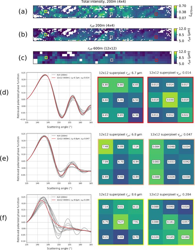
B. A. McBride et al.: Spatial distribution of cloud droplet size properties from AirHARP measurements 1783
2 may be higher than 1.5, but the RMSE threshold can
χred
still find a solution if the measurement residuals are not too
far from the best-fit curve. This may also occur for observa-
tions of multi-layer cloud fields. Because the χred 2 depends
strongly on the uncertainty of the individual measurements,
there is also a possibility that pixels that represent narrow
size distributions may give a valid retrieval, while producing
2 values beyond 1.5. Figure 6a is one such example. The
χred
cloudbow oscillations are well-defined and AirHARP data
2 is 2.52. While the
clearly capture the pattern, though the χred
error bar on several AirHARP data points does not touch the
best-fit polarized reflectance, the overall curve fit does repre-
sent the information content in the measurement. It is there-
fore important to include the RMSE as a two-factor authenti-
cation. Third, Breon and Goloub (1998) noted that secondary
and tertiary scattering events in the primary bow region (137–
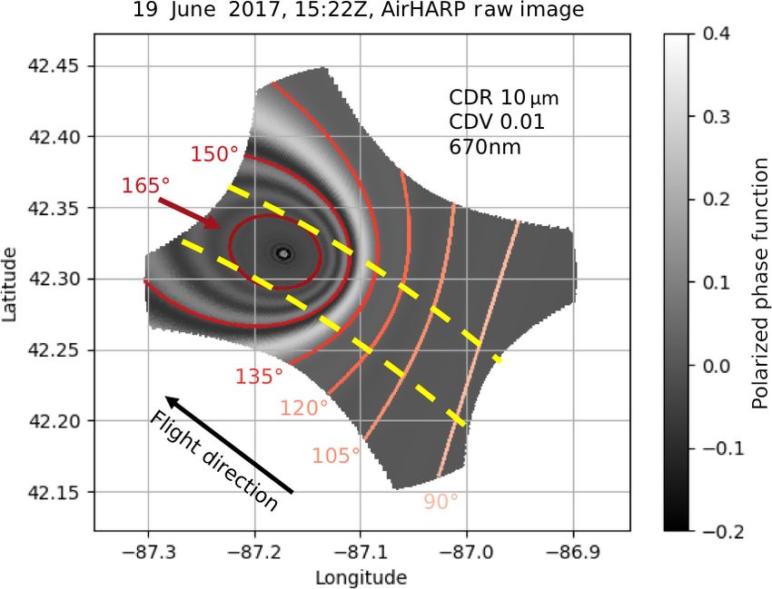
145◦ in scattering angle) can widen the polarized signal here Figure 3. The scattering angle coverage typical of an instantaneous
relative to Mie simulations. Here, the RMSE may preserve AirHARP wide-FOV observation, projected to simulate a scene
a strong fit in the supernumerary region, where the majority over Lake Michigan on 19 June 2017 at 15:22 Z (a). The cloudbow
of the DSD information content lies, even if the χred 2 is be- in this simulation represents a simulated cloudbow at 670 nm, with
yond our threshold. These diagnostics also account for any CDR 10um and CDV 0.01, with scattering angle isolines from 90
to 165◦ shown (solid lines). Note that the cloudbow pattern occurs
artifacts that arise from rotating our reference frame of polar-
within 135–165◦ in scattering angle, and the location of the cloud-
ization into the scattering plane and retrievals that converge
bow in the FOV depends on time of day, flight orientation, and solar
artificially to the edges of the LUT. When the uncertainty is geometry. Note that the only portion of the image that is eligible for
high relative to the measurement, both χred 2 and RMSE will
retrieval lies inside the region defined by along-track lines tangent
also be high and the retrieval will be rejected if both values to the 165◦ scattering angle isoline (yellow dotted lines).
exceed their expected ranges. More details on some of these
effects are discussed in Sect. 6.
The focus of this paper is on the application of AirHARP
cloud datasets and not the retrieval algorithm itself; therefore, 10 µm and CDV of 0.01, with the same solar and viewing
we use a simple treatment of the classic parametric model. geometry of the LMOS observation. Note that this is the
This retrieval will be extended to multi-modal DSDs and take scattering angle coverage for a single snapshot, and when
into account both multi-angle and multi-spectral sampling in AirHARP flies over a cloud deck, it is taking two snapshots
future studies. a second. This means a different portion of the detector is
imaging the same cloud target from image to image, which
also suggests that the scattering angle observed at the tar-
4 Hyper-angular polarized cloud retrievals from get changes image to image as well. From the perspective of
AirHARP the detector, the target travels from the front of the detector
to the back during a full angle observation, reflecting solar
Before we discuss how the retrieval is applied to the light at different scattering angles as the instrument flies over
AirHARP data, we will first walk through an AirHARP mea- it. Therefore, only along-track pixel columns inside the yel-
surement. As the AirHARP instrument images a scene for a low dotted lines in Fig. 3 contain pixels that are eligible for
particular solar geometry, each view sector captures a range a polarimetric DSD retrieval. This work does not perform a
of scattering angles unique to each of the 120 view sec- retrieval on any targets observed outside these lines. Outside
tors and wavelengths. Figure 3 shows an example of the these lines, the reduced scattering angle coverage at the up-
AirHARP instantaneous scattering angle coverage for a sim- per end of the cloudbow range begins to truncate the signal
ulated observation at 15:22 UTC over Lake Michigan on from the supernumerary bows. Because the majority of the
19 June 2017 during the NASA Lake Michigan Ozone Study size distribution information is encoded in the supernumer-
(LMOS) field campaign. This target was chosen because of ary bows (145–165◦ ), it is important that the full scattering
the cloud conditions present during the observation, and the angle range is preserved.
solar geometry allows for retrievals across the swath and Figure 4 shows the view sector isolines of AirHARP over
along the entire length of the observation. Figure 3 shows a the same snapshot from Fig. 3. The AirHARP wide FOV cov-
simulated cloudbow as it would appear in a single AirHARP ers view sectors from ±57◦ , but note that the cloudbow only
snapshot if the entire detector was capable of sampling at covers a subset of these. Push brooms are made from individ-
670 nm. This cloud field was simulated using a CDR of ual view sectors as the instrument flies over the cloud field.
www.atmos-meas-tech.net/13/1777/2020/ Atmos. Meas. Tech., 13, 1777–1796, 2020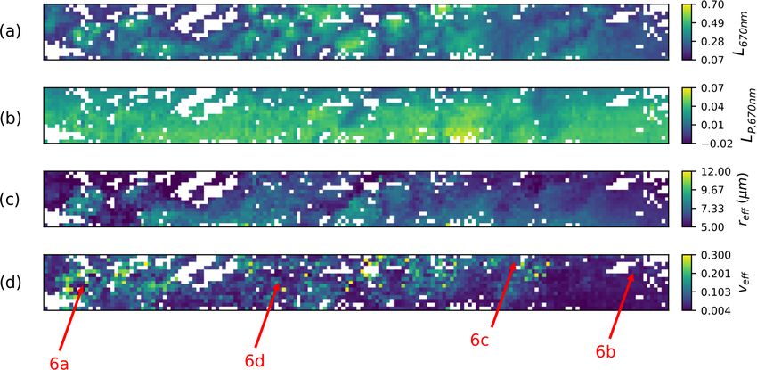
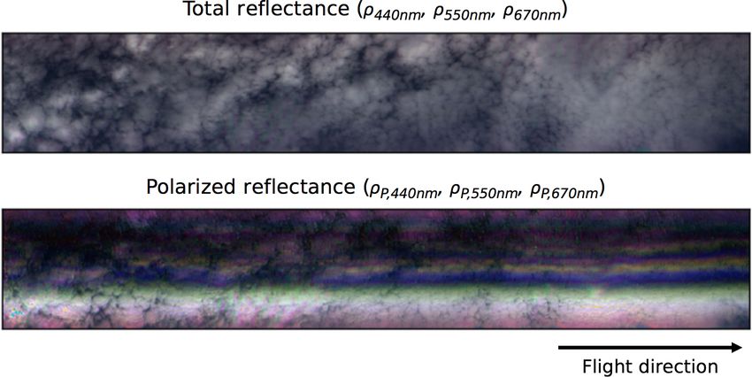
1784              B. A. McBride et al.: Spatial distribution of cloud droplet size properties from AirHARP measurements

Figure 4. The same simulation as Fig. 3, now with along-track view sector (zenith angle) isolines (a). A push broom is made when a view
sector images consecutive information along-track, shown for seven view sectors, separated by 7.5◦ each (b). Because cross-track pixels
represent a cross section of the cloudbow, they are also proxies for scattering angle. Note that the cloudbow distribution is different for each
view sector push broom. Since each push broom is projected on a common grid, any pixel or superpixel in common to all of the views
can generate a discrete polarized structure. This measurement can be compared to Mie simulations to retrieve CDR and CDV at the target
resolution.

Figure 4b shows examples of push brooms built from cloud-                 2 times the standard deviation of the polarized reflectance
bow content in Fig. 4a isolines. If AirHARP was to fly over               measured by the pixels inside the superpixel bin. Superpixels
this simulated field, the cloudbow would transition from a                are constructed from finer-resolution native pixels to increase
concentric space in the raw image to a linear one in the push             SNR and mitigate other potential artifacts in the data. These
brooms. This occurs because each view sector only observes                artifacts will be discussed in Sect. 6. Note that Fig. 6a and b
a specific cross section of the cloudbow at any one time, and             both represent narrow DSDs with low CDV values, though
the structure of the cross section is maintained due to the               the difference in CDR causes a shift in the location of the ob-
geometry of a single view sector. Figure 5 shows the actual               served supernumerary bows. Figure 6c and d are wider DSDs
AirHARP observation during LMOS, in total (top) and po-                   with higher CDV values, with eroded supernumeraries. As
larized reflectance (bottom), at view sectors near +38◦ dur-              the DSDs become wider and wider, this retrieval method be-
ing the time and day used to simulate Figs. 3 and 4. The                  comes less and less accurate at inferring CDV, as the super-
red–green–blue (RGB) composite image of the polarized re-                 numerary region becomes monotonic and linear. The CDR
flectance displays the cross-track cloudbow structure of the              values retrieved in Fig. 6 are typical of non-precipitating stra-
segment near +38◦ in the Fig. 4b simulation. The polarized                tocumulus cloud fields (Pawlowska et al., 2006), and CDV
reflectance image shows the wavelength dependence in the                  values are similar to those found by Alexandrov et al. (2015)
polarized cloudbow structure, which is absent from the total              using RSP measurements over marine stratocumulus.
reflectance image. Also, the appearance of the cloudbow in                   The hyper-angular retrieval requires data that are captured
this push broom is highly variable compared to the simula-                over a short time window as AirHARP flies over a cloud: it
tion in Figs. 3 and 4, which reflects the heterogeneity in the            takes time for the AirHARP backward angles to image the
cloud field seen in total reflectance.                                    same location on the ground as the forward angles. The dif-
   Since a single target moves across the detector in consec-             ferences in time depend on the instrument-level flight speed
utive snapshots, there will always be a location in each of the           and the difference in altitude between the instrument and tar-
120 push brooms that represents that target on the ground,                get. For the LMOS campaign, the difference between ±57◦
and any cloudbow target appearing in multiple sector views                observations was 112 s (∼ 2 min) for a nominal UC-12 flight
having sufficient scattering angle range can be used in a po-             speed of 133 m s−1 at 4.85 km of altitude above the cloud
larimetric cloud DSD retrieval. Figure 6 shows several ex-                deck. Note that the actual aboveground altitude was 8 km,
amples of an AirHARP 200 m superpixel retrieval of differ-                but the cloud deck was geolocated to be 3150 m on average.
ent regions of the LMOS cloud field shown in Fig. 5 using                 Therefore, the hyper-angular retrieval requires cloud con-
hyper-angular, co-located information. Error bars represent               stancy over this time interval. If we only include the angles

Atmos. Meas. Tech., 13, 1777–1796, 2020                                                       www.atmos-meas-tech.net/13/1777/2020/
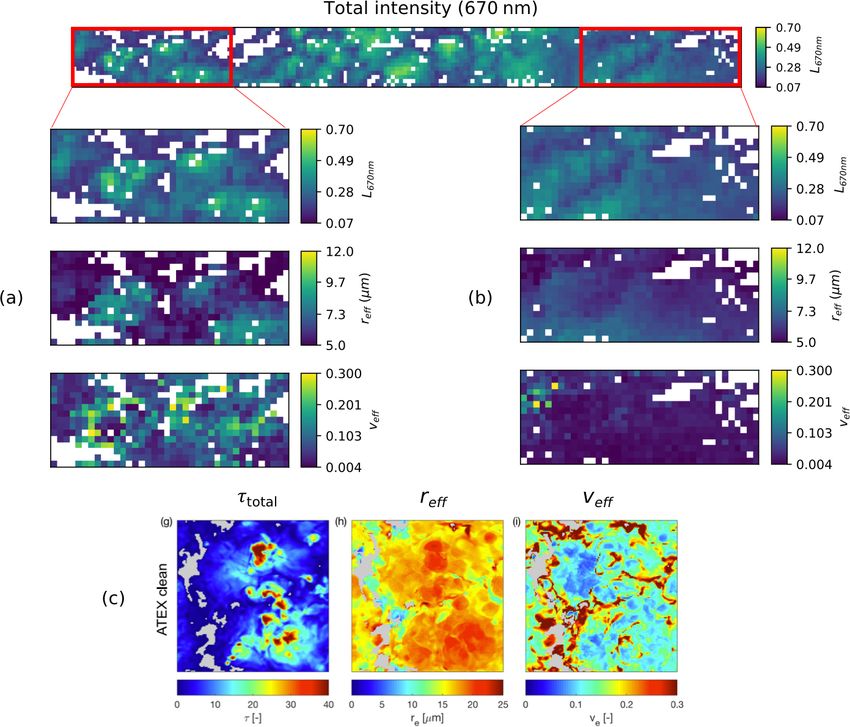
B. A. McBride et al.: Spatial distribution of cloud droplet size properties from AirHARP measurements                                  1785

Figure 5. AirHARP data taken at the same time, location, and geometry as Figs. 3 and 4 reveal a heterogenous cloud field in total re-
flectance (a) and a cloudbow in polarized reflectance (b). The linear distribution of cloudbow oscillations is heterogenous compared to the
Fig. 4b simulation and reflects the variability in the cloud field. Both images are RGB composites of push brooms from 440, 550, and 670 nm
view sectors near +38◦ , presented without axes for visual purposes only. A single gridded pixel in this image represents 50 m, and the scene
stretches approximately 37 km along-track by 5 km cross-track.

used in the cloudbow retrieval, the time interval between                olution (200 m), and the polarized radiances (LP,670 nm ) are
the views with the largest angular separation is reduced to              converted into polarized reflectances via Eq. (3) before en-
a minute. A study with the HARP CubeSat at an estimated                  tering the retrieval process. The portion of the image capable
400 km orbital altitude and 7.66 km s−1 ISS speed requires               of retrieval stretches 34 km along-track and 3 km cross-track.
∼ 160 s (∼ 2.5 min) for the same full-angular coverage over                 The distribution of CDR and CDV in AirHARP data is
the same cloud target. In this way, the HARP hyper-angular               consistent with prior studies and physical phenomena. Be-
retrieval still requires an assumption of homogeneity in a               cause the cloud case observed during LMOS was heteroge-
short time window over a narrow pixel.                                   nous, there are several examples of how cloud substructure
   With this in mind, any liquid water cloud pixel in the                can give different retrievals. Figure 8 takes a few areas from
AirHARP wide FOV that samples scattering angles be-                      Fig. 7 and zooms in on their retrieval results. Figure 8b shows
tween 135 and 165◦ can be used to retrieve CDR and CDV.                  a uniform sector of the cloud field, described this way be-
This constraint is used in several other polarimetric stud-              cause of its visual homogeneity in both intensity and CDR as
ies, though with a slight discrepancy on the start of the                well as the narrow and consistent CDV retrievals over many
lower bound (Di Noia et al., 2019; Alexandrov et al., 2015).             pixels. The results here suggest that the supernumerary bows
Shang et al. (2015) found that using a 137–165◦ scatter-                 are well-defined and the cloud pixels have narrow size dis-
ing angle range as opposed to the operational POLDER                     tributions. Figure 8a shows a region of the same leg that is
145–165◦ improved many of the CDR and CDV retrievals,                    heterogeneous in CDV, and the intensity and CDR distribu-
specifically for CDR > 15 µm (Shang et al., 2019). The up-               tion suggest that this area is a region of convection: larger
per bound of 165◦ is consistent between studies dating back              CDR in the cloud core, or central area of the cloud, and
to Breon and Goloub (1998): the bulk of the microphys-                   smaller CDR retrieved on the periphery, where the intensity
ical information lies in the supernumerary bows, and the                 is lower. We will look at this phenomenon in more detail in
assumption of a structureless Usca breaks down after this                the AirHARP data in the sections below. Here we point out
point (Alexandrov et al., 2012a). Figure 7 shows an exam-                that large-eddy simulations (LESs) of similar heterogenous
ple of how individual pixel retrievals generate a spatial dis-           clouds show similar spatial distributions of intensity, CDR,
tribution of CDR and CDV for those that access this cloud-               and CDV (Miller et al., 2018), with one representative case
bow scattering angle range. Each pixel is first conservatively           shown in Fig. 8c. Miller et al. (2018) simulate LES clouds
masked for non-clouds using the nadir 670 nm intensity push              using vertical weighting functions that take into account the
broom (−0.003◦ VZA) using a conservative threshold of                    distribution of reflectance at the edges of the cloud, echoing
0.06 W m−2 sr−1 nm−1 to avoid cloud holes and views of                   theoretical recommendations made by Platnick (2000).
Lake Michigan below. All pixels are aggregated to 4 × 4 res-

www.atmos-meas-tech.net/13/1777/2020/                                                       Atmos. Meas. Tech., 13, 1777–1796, 2020
1786 B. A. McBride et al.: Spatial distribution of cloud droplet size properties from AirHARP measurements
Figure 6. Several examples of the traditional parametric fit retrieval applied to AirHARP hyper-angular polarized reflectance measurements
for 200 m superpixels. Panels (a) and (b) signify narrow DSDs with small CDV values. In panels (c) and (d), the eroded supernumerary bows
2 in
suggest wider DSDs. Error bars represent the 2σ standard deviation of the measurements inside the superpixel. Note that while the χred
(a) is larger than our 1.5 threshold, the overall fit to measurement generates a valid RMSE.
While these simulations can assume any resolution, the 5 Spatial scale analysis
AirHARP retrievals are performed at 200 m in this study and
even coarser resolutions from space. The small-scale vari- Because the AirHARP retrievals of CDR and CDV are im-
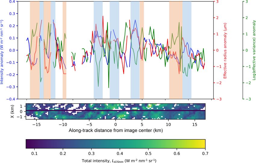
ability in the cloud field can also be missed by MODIS radio- ages, any sector of the cloud field can be analyzed by taking
metric analyses, for example, which assumes constant CDV a transect of pixels along- or cross-track. In Fig. 9, we take
in their droplet size retrieval. This is one of the strongest ben- a 34 km pixel transect of the cloud field (shown in the inset
efits of polarized cloud retrievals: a quantitative measurement intensity image with a black line) and compare the anomaly
of heterogeneity through CDV information, which is not pos- from the mean along the track for intensity, CDR, and CDV.
sible with traditional radiometric methods. This has serious The CDV is log-scaled to linearize its several orders of mag-
implications for climate in terms of quantifying cloud devel- nitude range. Positive CDR anomalies describe larger droplet
opment, brightness, and lifetime, aerosol–cloud interaction, sizes, and positive CDV anomalies correspond to wider dis-
and reducing the uncertainty in global radiative forcing due tributions. Any position along the transect of the cloud field
to clouds and aerosols. In the following section, we explore lines up exactly with three unique points in the plot, and
how we can extend the AirHARP spatial retrievals of CDR the correlation between the three curves suggests information
and CDV to study changes in size properties along the cloud about the nature of the cloud field. It is important to note that
field and the impact of resolution on the retrieval itself. we are using the cloud intensity as a proxy for COT, which
is orthogonal to CDR (Nakajima and King, 1990). In some
locations in the plot, intensity (COT) and CDR are correlated
with each other and anticorrelated with CDV. Blue blocks de-
Atmos. Meas. Tech., 13, 1777–1796, 2020 www.atmos-meas-tech.net/13/1777/2020/B. A. McBride et al.: Spatial distribution of cloud droplet size properties from AirHARP measurements 1787 Figure 7. Nadir push-broom images for 670 nm of total intensity (a) and polarized intensity (b), as well as for the retrieved CDR (c) and CDV (d) for 200 m (4 × 4) gridded superpixels with access to 135–165◦ in scattering angle using hyper-angular co-located data. Quality- flagged retrievals are screened out (white). Note that the polarized reflectance is smoother compared with the reflectance image, and both represent nadir (−0.003◦ ) view sector push brooms. The general locations of each retrieval from Fig. 6 are identified in red. The scene stretches 3 km cross-track and 34 km along-track. fine unambiguous locations in the cloud field where intensity collisional processes (de Lozar and Muessle, 2016). On the and CDR have positive anomalies while the CDV anomaly periphery, evaporation removes smaller droplets, and at the is negative, whereas orange blocks give the opposite: inten- same time, the entrainment of warm air and/or aerosol here sity and CDR are negative and CDV is positive. If we de- may enhance droplet growth. There are many competing the- fine cloud cores as the pixels brightest in intensity (blue) and ories as to the net effect of aerosol entrainment on droplet cloud peripheries as darkest in intensity (orange) then cloud growth (Small et al., 2009, and references therein), but these cell sizes appear to be of the order 1–4 km, both comparable two opposing effects may create a larger DSD variance on to and slightly larger than traditional MODIS cloud droplet the periphery. Alexandrov et al. (2015) and Platnick (2000) size retrieval products (1 km). Comparison to the traditional suggest that CDR changes occur vertically in the cloud pe- cloud product resolution is notable because, in some regards, riphery. Therefore, multi-angle polarimeters that can sample the 1 km resolution is adequate to resolve cloud microphysics deeper into the periphery could retrieve a larger CDV in these of the cloud cores. However, when cores and peripheries are areas. The above LES study of broken marine stratocumulus found in the same 1 km pixel, issues in separating DSDs will by Miller et al. (2018) also shows higher CDV (lower CDR) arise. Since AirHARP is an aircraft instrument and flies be- in the cloud periphery and lower CDV (higher CDR) in cloud neath 20 km, its resolution will be better than an equivalent cores, as shown in Fig. 8c. In the present study, all of these AirHARP instrument in space, so this fine-scale variability processes cannot be decoupled, but these promising results will likely not be captured by HARP CubeSat or HARP2. show that AirHARP retrievals are consistent with current re- Regardless, this result emphasizes the importance of small- search and theories of cloud microphysics. scale sub-kilometer sampling of cloud fields because cloud Furthermore, the AirHARP pixel resolution can be de- heterogeneity and microphysical processes may be lost in the graded and used to understand the effect of sub-pixel vari- large spatial resolutions of spaceborne instruments. ability on the DSD retrieval itself, as shown in Fig. 10. Fig- There are physical explanations for the relationships we ure 10a and b are repeated from Fig. 7a and b, and both rep- see between intensity, CDR, and CDV on the spatial scales resent the 200 m CDR retrieval, while Fig. 10c shows the of Fig. 9. Liquid water droplets that form at the base of adi- CDR product at 600 m resolution. To calculate the 600 m abatic clouds, such as cumulus and stratocumulus, see their product, the gridded polarized reflectance data at the original largest sizes at cloud top (Platnick, 2000) and further grow 50 m resolution are aggregated into 600 m superpixels. Next, by longwave radiative cooling, small-scale turbulence, and the superpixels pass through a screening process: this elimi- www.atmos-meas-tech.net/13/1777/2020/ Atmos. Meas. Tech., 13, 1777–1796, 2020
1788             B. A. McBride et al.: Spatial distribution of cloud droplet size properties from AirHARP measurements

Figure 8. A zoom of two sectors of the AirHARP polarized cloud retrieval for the LMOS cloud field. The intensity image (top) shows
both a heterogeneous (a) and a homogenous region (b), defined by the distribution of CDR and CDV, as well as visual cues from the total
reflectance. Large-eddy simulations of clean clouds (c), performed by Miller et al. (2018), show that high CDV (veff ) and low CDR (reff )
typify cloud periphery regions, and low CDV and higher CDR occur in the core of the clouds. Similar CDV–CDR relationships are seen in
the AirHARP retrievals (a) at 200 m resolution.

nates low-intensity superpixels that represent cloud holes and         represent the retrieved CDR (middle column) and CDV (right
marginal situations. Third, the superpixels enter the retrieval        column) for the colored superpixel boxes located in Fig. 10a–
process. Thus, Fig. 10c is not a resampling of Fig. 10b but a          c. The 600 m CDR or CDV result is given in the title above
new retrieval using a different resolution as input. This study        each box and represents the retrieval for the entire nine-box
does not examine the effect of cloud screening at the different        square underneath, whereas the 200 m CDR or CDV results
resolutions, only the effect of the degraded resolution using          are shown inside each colored sub-box.
pixels that have been properly identified as clouds at the finer          Figure 10d shows that the narrow DSD retrievals are ro-
resolution.                                                            bust against resolution degradation; if we take the 200 m re-
   The plots on the left-hand side of Fig. 10d–f are the re-           trievals as truth, the 600 m result agrees within community
trieved P12 curves, which emphasize how the nine 200 m re-             standards (10 % σCDR and 50 % σCDV ; Mishchenko et al.,
trievals, shown as gray lines, compare to the single 600 m             2004). The 600 m P12 resembles the 200 m P12 curves, both
retrieval, which is shown as a red line. The two boxes to the          in the location of supernumerary peaks and overall struc-
right of each of the retrieved P12 curve plots in Fig. 10d–f           ture. Figure 10e shows a retrieval that appears to represent

Atmos. Meas. Tech., 13, 1777–1796, 2020                                                   www.atmos-meas-tech.net/13/1777/2020/
B. A. McBride et al.: Spatial distribution of cloud droplet size properties from AirHARP measurements                                 1789

Figure 9. Analysis of intensity (blue), CDR (red), and log (CDV) (green) anomalies from the mean following the black transect along the
nadir intensity push broom for a segment of the cloud field measured by AirHARP (bottom). Using the spatial distribution of intensity
as a proxy for cloud optical thickness (COT), we can visually identify what appear to be cloud cores (blue blocks) and cloud periphery
(orange blocks) regions. CDV trends are opposite to intensity and CDR in both regions, but wider DSDs with smaller CDR appear at cloud
peripheries, while larger CDRs with narrow DSDs appear in cloud cores. The label X to the left of the intensity image is an abbreviation for
cross-track distance from the image center line.

the cloud periphery, as the intensity image shows the ap-               was performed with RSP single-pixel sampling, as it is here
pearance of a cloud cell near the superpixel. Here, the CDR             with AirHARP data. Figure 10f shows another retrieval done
retrieval gives higher values in the center of the structure            close to the cloud periphery, but this time, the retrieved 200 m
and smaller values on the sides, consistent with prior stud-            P12 curves show a wider spread of CDV values compared to
ies. Figure 10e shows two conflicting P12 regimes. Here,                the results shown in Fig. 10d–e.The retrieved 600 m fit gen-
200 m DSDs with CDR between 6.6 and 7.5 µm separate into                erates a curve that does not represent any of the sub-pixel re-
two modes: CDV > 0.08 and CDV between 0.048 and 0.028.                  sults. The consequence is a broad 600 m CDV that reflects the
While the primary bow around 143◦ is preserved between                  200 m variability but not the mean magnitude of the nine sub-
retrieval scales, the 600 m retrieval gives a CDV of 0.047, a           pixels, as the 600 m retrieved value for CDV is 0.284, while
value that appears to represent the mean of the nine pixels             the nine individual pixels return values 0.086 to 0.186. Here,
but satisfies neither regime. Shang et al. (2015) and Miller            the sub-pixel variability smears out the supernumerary bows.
et al. (2018) show similar results in theoretical and obser-            This result is a well-known consequence of mixed DSDs in a
vational mixed DSDs. Note that the combination of gamma                 large superpixel, but it does not provide any information as to
distributions inside a superpixel is not itself a gamma distri-         which parts of the cloud inside the superpixel contain narrow
bution, though retrievals that contain sub-pixel heterogeneity          vs. wider DSDs. The interpretation of CDR and CDV at large
in the DSD still attempt to infer gamma distribution proper-            pixel sizes is still widely debated, but fine-resolution spatial
ties from a signal that may not represent one (Shang et al.,            data provided by AirHARP and its retrievals can provide a
2015). The rainbow Fourier transform method (Alexandrov                 meaningful advancement in this direction.
et al., 2012b) may distinguish these two modes at the 600 m
scale, but the result could not be independently validated if it

www.atmos-meas-tech.net/13/1777/2020/                                                      Atmos. Meas. Tech., 13, 1777–1796, 2020
You can also read