Development of a MetUM (v 11.1) and NEMO (v 3.6) coupled operational forecast model for the Maritime Continent - Part 1: Evaluation of ocean ...
←
→
Page content transcription
If your browser does not render page correctly, please read the page content below
Geosci. Model Dev., 14, 1081–1100, 2021
https://doi.org/10.5194/gmd-14-1081-2021
© Author(s) 2021. This work is distributed under
the Creative Commons Attribution 4.0 License.

Development of a MetUM (v 11.1) and NEMO (v 3.6) coupled
operational forecast model for the Maritime Continent –
Part 1: Evaluation of ocean forecasts
Bijoy Thompson1 , Claudio Sanchez2,3 , Boon Chong Peter Heng3 , Rajesh Kumar3 , Jianyu Liu3 , Xiang-Yu Huang3 , and
Pavel Tkalich1
1 Tropical Marine Science Institute, National University of Singapore, Singapore 119222, Singapore
2 Met Office, Exeter, EX1 3PB, United Kingdom
3 Centre for Climate Research Singapore, Meteorological Service Singapore, Singapore 537054, Singapore

Correspondence: Bijoy Thompson (bijoymet@gmail.com)

Received: 29 September 2020 – Discussion started: 19 October 2020
Revised: 15 December 2020 – Accepted: 29 December 2020 – Published: 23 February 2021

Abstract. This article describes the development and ocean         1   Introduction
forecast evaluation of an atmosphere–ocean coupled predic-
tion system for the Maritime Continent (MC) domain, which          Dynamical processes and flux exchanges between Earth sys-
includes the eastern Indian and western Pacific oceans. The        tem components are better represented in coupled mod-
coupled system comprises regional configurations of the at-        elling systems rather than the single-component models (e.g.
mospheric model MetUM and ocean model NEMO at a uni-               Meehl, 1990). Hence, coupled models, particularly with dy-
form horizontal resolution of 4.5 km × 4.5 km, coupled us-         namically interactive atmosphere, ocean, land surface, and
ing the OASIS3-MCT libraries. The coupled model is run             sea ice models, are increasingly employed for climate re-
as a pre-operational forecast system from 1 to 31 Octo-            search as well as operational forecast applications (e.g.
ber 2019. Hindcast simulations performed for the period            Miller et al., 2017; Lewis et al., 2018, 2019a). The atmo-
1 January 2014 to 30 September 2019, using the stand-alone         sphere and ocean are two major components of the Earth’s
ocean configuration, provided the initial condition to the         climate system, and interactions between these two systems
coupled ocean model. This paper details the evaluations of         are key drivers of climate and weather. In the past, efforts to-
ocean-only model hindcast and 6 d coupled ocean forecast           ward the development of atmosphere–ocean coupled models
simulations. Direct comparison of sea surface temperature          were largely constrained by their high computational require-
(SST) and sea surface height (SSH) with analysis, as well as       ments, limited understanding of air-sea coupled processes,
in situ observations, is performed for the ocean-only hindcast     and lower computational efficiency (Meehl, 1990). During
evaluation. For the evaluation of coupled ocean model, com-        the last 3 decades, there have been significant advancements
parisons of ocean forecast for different forecast lead times       in the computational power of supercomputers and the com-
with SST analysis and in situ observations of SSH, temper-         putational efficiency of atmosphere–ocean circulation mod-
ature, and salinity have been performed. Overall, the model        els. Presently, global atmosphere–ocean–wave–land surface–
forecast deviation of SST, SSH, and subsurface temperature         sea ice coupled operational forecasts are available at spa-
and salinity fields relative to observation is within acceptable   tial resolutions of 0.1◦ in the Integrated Forecast Systems
error limits of operational forecast models. Typical runtimes      (IFS) developed by the European Centre for Medium Range
of the daily forecast simulations are found to be suitable for     Weather Forecasting (ECMWF) to 0.25◦ in the Global Fore-
the operational forecast applications.                             cast System (GFS) developed by the National Center for En-
                                                                   vironmental Prediction (NCEP). Moreover, the accessibility
                                                                   of high-performance computers (HPCs) to researchers has
                                                                   considerably increased in the last decade. Several regional

Published by Copernicus Publications on behalf of the European Geosciences Union.
1082                                                  B. Thompson et al.: Coupled forecast model for the Maritime Continent

                                                                      of atmospheric and ocean hindcast and forecast significantly
                                                                      improves when the simulations are performed using coupled
                                                                      models (Xue et al., 2014; Thompson et al., 2018; Lewis et
                                                                      al., 2019a). There have been a few coupled modelling stud-
                                                                      ies over the MC focusing on the climate and weather research
                                                                      or short-range atmosphere–ocean forecasting (e.g. Aldrian
                                                                      et al., 2005; Wei et al., 2014; Li et al., 2017; Thompson et
                                                                      al., 2018). Recently, Xue et al. (2020) presented a review of
                                                                      atmosphere–ocean coupled modelling studies over the MC
                                                                      region.
                                                                         Besides coupling, the model skill in simulating atmo-
                                                                      sphere and ocean state shows a strong relation to the grid
                                                                      resolution also (e.g. Li et al., 2017). Local mesoscale pro-
                                                                      cesses (e.g. land and sea breezes) also play an important role
                                                                      in the adequate simulation of upscale processes such as the
                                                                      MJO (Birch et al., 2016). Convection plays a fundamental
Figure 1. Bathymetry and orography (in metres) of the Maritime        role, either locally or embedded in bigger envelopes such as
Continent from GEBCO 2014 data: MC coupled model domain               the MJO, influencing the diurnal cycle of precipitation and
(black box), western Maritime Continent domain in Thompson et         moving squall lines (Love et al., 2011). Therefore, the simu-
al. (2018) (red box), and domain used for ocean forecast evaluation   lation of weather and climate processes over the MC requires
in present study (purple box).                                        sufficient resolution to resolve these scales and their inter-
                                                                      actions. Generally, a horizontal resolution of approx. 4 km,
                                                                      so-called convection permitting, has been effective in repre-
and global atmosphere–ocean coupled modelling systems                 senting fine-scale processes over the MC (Love et al., 2011;
have been developed worldwide during this period (see re-             Birch et al., 2014, 2016; Vincent and Lane, 2017). The first
views by Giorgi and Gutowsky, 2015, and Xue et al., 2020).            attempt towards the development of a convection-permitting
   The tropical region lying between the eastern Indian               atmosphere–ocean coupled model over the MC was under-
Ocean and western Pacific Ocean, encompassing the Malay               taken by Thompson et al. (2018, hereafter T18). T18 used a
Peninsula, Philippine Archipelago, Indonesian Archipelago,            regional version of the UK Met Office Unified Model (Me-
and surrounding oceanic and island region is generally re-            tUM) atmospheric model and Nucleus for European Mod-
ferred to as the Maritime Continent (MC). This region is              elling of the Ocean (NEMO) ocean model configured for
characterised by complex orography and shallow seas inter-            the western MC (WMC). For simplicity, the WMC coupled
connected by numerous straits (Fig. 1). The MC region is              model configuration used in T18 is referred to as WMCao
characterised by strong atmosphere–ocean coupled processes            hereafter. The atmosphere and ocean components of WMCao
across multiple timescales. The El Niño–Southern Oscilla-             were configured for the same domain and similar horizon-
tion (Bjerknes, 1969) and the Indian Ocean Dipole–Zonal               tal resolution of 4.5 km × 4.5 km (Fig. 1). The model reso-
Mode (Saji et al., 1999; Webster et al., 1999) represent two          lution is fine enough to represent the complex coastal geog-
dominant climate modes of variability that influence the MC           raphy, ocean bathymetry at shallow oceans and straits, and
on inter-annual timescales. Meanwhile, the monsoons and               orographic features, such as mountain ranges, with enormous
Madden Julian Oscillation (MJO, Madden and Julian, 1994)              influences in local weather (e.g. Bukit Barisan in Sumatra or
manifest the coupled processes over the MC in seasonal and            the Sierra Madre in Luzon).
intra-seasonal scales, respectively. Because of its geographi-           Work to develop and perform a first-hand evaluation of the
cal location in the middle of the Indo-Pacific warm pool and          WMCao , described in T18, was a preliminary step aimed to
in the ascending branch of global atmospheric Walker cir-             establish a high-resolution atmosphere–ocean coupled model
culation, the MC has been identified as an area of climatic           focusing on the Southeast Asian region for both operational
importance both in regional and global environments (Neale            forecasts and climate research applications. Since the over-
and Slingo, 2003; Qu et al., 2005).                                   all objective of the development was to simulate both atmo-
   The development of regional coupled models is mainly               spheric and oceanic variables, the coupling has provided a
driven by the idea that by resolving fine-scale orographic,           better consistency between the atmospheric conditions and
ocean circulation, and coastal ocean features, a more accurate        that of the ocean underneath rather than employing stand-
representation of atmosphere–ocean dynamics and coupled               alone models. The case studies conducted as part of the
processes can be achieved. The prediction of atmospheric              WMCao evaluation suggested that the zonal extent of the
and oceanic variables over the MC is challenging because of           domain might not be sufficient for an accurate prediction
its complex geography, strong air–sea coupling, and remote            of weather events such as cold surges or typhoons. For in-
ocean influences. Earlier studies suggested that the accuracy         stance, cyclogenesis inside the South China Sea (SCS) is

Geosci. Model Dev., 14, 1081–1100, 2021                                               https://doi.org/10.5194/gmd-14-1081-2021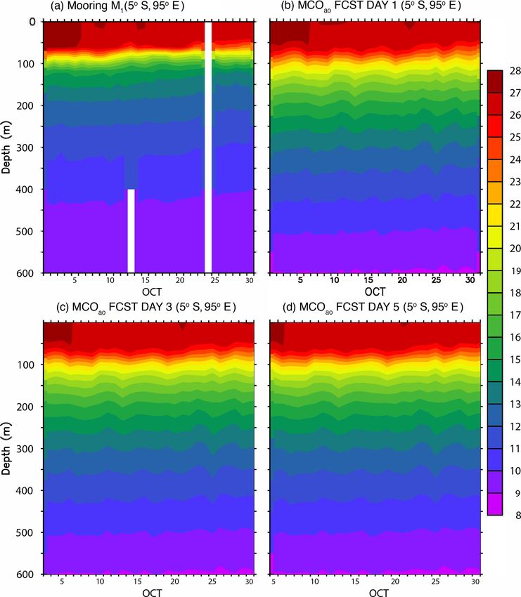
B. Thompson et al.: Coupled forecast model for the Maritime Continent                                                       1083

relatively low and most of the cyclones and typhoons that           sitioned roughly between 10◦ N, 140◦ E and 60◦ N, 150◦ E
appear over the SCS originated in the northwestern Pacific          (Gvirtzman and Stern, 2004). The model eastern boundary
Ocean (e.g. Ling et al., 2011). The northern Pacific Ocean          is limited to 141◦ E to avoid numerical instabilities that may
region between 100◦ E and 180◦ E/W is the most active trop-         arise due to steep bathymetric slopes such as the Mariana
ical cyclone basin on Earth and it accounts for about one-          Trench. Both the atmospheric and ocean components of the
third of the world’s tropical cyclones annually (e.g. Lee et al.,   coupled system are selected to have the same domain. The
2020). Hence, rather than internally coupled dynamics, the          horizontal resolution of the MC coupled model remained
predicted track and typhoon characteristics are dominantly          the same (4.5 km × 4.5 km) as that of the WMCao . The MC
driven by the lateral boundary conditions (LBCs) in WMCao .         atmosphere–ocean coupled model configuration is referred
Similarly, the simulation of MJO- and cold-surge-related            to as MCao in this paper.
weather parameters may also be heavily influenced by LBCs.
Hence, to address the issues encountered in T18 and incor-          2.2   Atmospheric model
porate the latest model scientific developments, the present
study aims to bring several key upgrades to the WMCao con-          The atmospheric component of T18 has been improved to
figuration, and test its feasibility in operational forecast ap-    employ the SINGV v5 science configuration described in
plication. The main updates to the coupled modelling system         Huang et al. (2019), which is similar to the Regional Atmo-
include extending the eastern boundary of the model domain          sphere and Land v1 in the Tropics (RAL1-T) configuration of
to the western Pacific Ocean, upgrading MetUM to the latest         MetUM (version 11.1) described in Bush et al. (2020). The
science configuration, and incorporating tide boundary forc-        model has been employed operationally by the Meteorolog-
ing into the NEMO.                                                  ical Service of Singapore since 2019 at a higher resolution
   This study presents details of the atmosphere–ocean cou-         (1.5 km) for the region 6◦ S to 8◦ N, 95◦ E to 109◦ E and is
pled prediction system developed for the MC and an evalu-           referenced in the literature as SINGV. The key differences of
ation of the ocean forecast from the system using a 6 d pre-        MCao atmospheric model component to T18 are as follows.
operational forecast for October 2019. Following the method           – Lateral boundary conditions are provided at 3-hourly
employed in many earlier coupled modelling studies (e.g. Li             frequency from the deterministic ECMWF forecasts in-
et al., 2014; Lewis et al., 2018), the evaluation of WMCao              stead of the MetUM global deterministic model. This
in T18 has been performed by using short case study simu-               change has led to a significant increase in precipitation
lations of selected weather events spanning over 5 d . In the           skill scores across all spatial scales and precipitation
present study, instead of case studies, we assess surface and           thresholds in SINGV (Huang et al., 2019).
subsurface oceanic variables predicted by the coupled system
across different forecast lead times.                                 – The model uses a prognostic cloud fraction and prog-
   The next section of this paper presents an overview of               nostic condensate scheme (PC2, Wilson et al., 2008) in-
the model setup, including a brief description of the model             stead of the diagnostic scheme of Smith (1990). This
domain, atmospheric, ocean, and coupled model configura-                change helped to reduce the occurrence of spurious con-
tions. A brief discussion of the pre-operational forecast sys-          vection with very high rainfall rates and resulted in a
tem setup is also presented. Section 3 provides the details of          better organisation of convection, as shown in Dipankar
datasets used for the atmosphere and ocean model forcing                et al. (2020).
and evaluation. Section 4 presents an assessment of the sea         The rest of the model formulations are similar to T18 and the
surface variables simulated by the stand-alone ocean model          SINGV configuration described in Huang et al. (2019). The
and both surface and subsurface ocean forecasts delivered by        main characteristics of the model are summarised below.
the MC coupled model. Finally, Sect. 5 summarises the re-
sults obtained from the study and suggests future develop-            – The dynamical core is the non-hydrostatic semi-
ments.                                                                  Lagrangian and semi-implicit Even Newer Dynamics
                                                                        for the General Atmospheric Modelling of the Envi-
                                                                        ronment (ENDGAME, Wood et al., 2014), with an
2     Model setup                                                       Arakawa-C staggered grid. The model time step is
                                                                        120 s.
2.1    Model domain                                                   – The model has a terrain-following vertical coordinate
                                                                        with a resolution of 80 levels and a top lid at 38.5 km.
The model domain extends from 18◦ S to 24◦ N and 92 to                  The vertical resolution is 5 m at the boundary layer and
141◦ E (Fig. 1) on a regular latitude–longitude grid that cov-          1.45 km below the model top, similar to the SINGV con-
ers most of the tropical regions of eastern Indian Ocean                figuration.
and western Pacific Ocean. The deepest oceanic trench on
Earth, known as the Mariana Trench, is located in the north-          – The boundary layer parameterisation is based on a
western Pacific Ocean. The crescent-shaped trench is po-                blending between the one-dimensional scheme of Lock

https://doi.org/10.5194/gmd-14-1081-2021                                              Geosci. Model Dev., 14, 1081–1100, 2021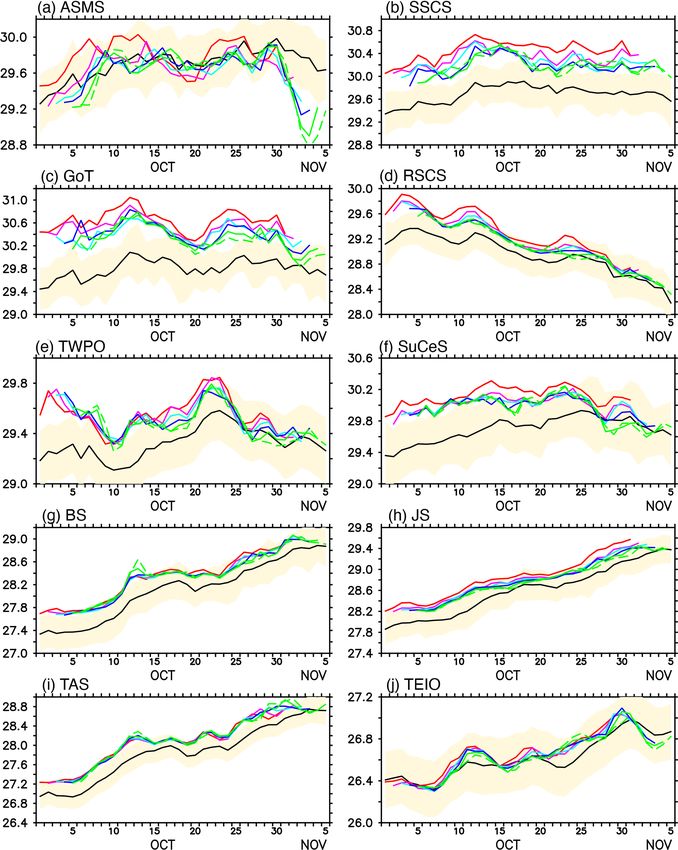
1084                                               B. Thompson et al.: Coupled forecast model for the Maritime Continent

      et al. (2001) and the three-dimensional Smagorinsky–        in MCao , whereas these coefficients were 1.2 × 10⁻⁴ and
      Lilly scheme (Lilly, 1962); this blending is described in   1.2 × 10⁻⁵ , respectively, in the WMCao . Additional vertical
      Boutle et al. (2014).                                       mixing resulting from internal tide breaking is parameterised
                                                                  in the model as proposed by St. Laurent et al. (2002). Both
  – The microphysics scheme is based on Wilson and Bal-           energy- and enstrophy-conserving schemes is used for the
    lard (1999) with prognostic rain formulation and im-          momentum advection. For lateral tracer diffusion, the Lapla-
    proved particle size distribution for rain as in Abel and     cian operator along geopotential levels with a coefficient of
    Boutle (2012).                                                20 m2 s−1 is used, while iso-level bi-Laplacian viscosity with
  – The radiation scheme is based on the Edwards and              a coefficient of −6 × 10⁷ m2 s−1 is applied for the momen-
    Slingo (1996) scheme, with six bands in the shortwave         tum mixing. An implicit form of non-linear parameterisation
    and nine bands in the longwave (Manners et al., 2011).        with a log layer formulation is used for the bottom drag coef-
                                                                  ficient computation. The minimum and maximum of the drag
  – The Joint UK Land Environment Simulator (JULES,               coefficient are set to 0.0001 and 0.15, respectively.
    Best et al., 2011) land surface scheme with 9 surface            At the lateral open-ocean boundaries, the flow relax-
    fraction types is also used.                                  ation scheme (FRS, Davies, 1976) is applied for the trac-
                                                                  ers and baroclinic velocities, while Flather boundary condi-
  – The moist conservation scheme is used as described in         tion (Flather, 1976) is used for the sea surface height (SSH)
    Aranami et al. (2015).                                        and barotropic velocities. One of the key updates to MCao
The Atmospheric component of the MCao employed in this            is the implementation of tide forcing at the lateral bound-
study is referred to as MCAao hereafter.                          aries and tide potential at the ocean surface. Due to certain
                                                                  numerical issues, the tide-related forcings are not included
2.3    Ocean model                                                in the WMCao . The tidal elevations and currents from finite-
                                                                  element solutions (FES2014b) data have been used for pro-
A regional version of Océan Parallélisé ocean engine within       viding the tidal harmonics at the lateral boundaries (Lyard et
the NEMO (version 3.6_stable, revision 6232, Madec et al.,        al., 2006). A total of 15 major tidal constituents (Q1, O1, P1,
2016) framework is employed as the oceanic component              S1, K1, 2N2, Mu2, Nu2, N2, M2, L2, T2, S2, K2, and M4)
of the MCao . NEMO is a primitive-equation, hydrostatic,          are included in the boundary forcing.
Boussinesq ocean model extensively used in climate and op-           Both coupled and uncoupled ocean model configurations
erational forecast applications. The MCao ocean configura-        are employed in the study. For uncoupled simulations, the
tion shares many features of its predecessor, WMCao . Hence,      air–sea heat fluxes are estimated using the Common Ocean-
only key features of the NEMO and main updates of MCao            ice Reference Experiment (CORE) bulk formulae (Large and
configuration are discussed here.                                 Yeager, 2004). However, a direct flux formulation is used in
   The model horizontal grid is in orthogonal curvilin-           the coupled ocean model. Monthly runoff climatology from
ear coordinates, with Arakawa-C grid staggering. The              Dai and Trenberth (2002) and chlorophyll monthly clima-
bathymetry of MCao is based on the General bathy-                 tology from SeaWiFS satellite observation are provided as
metric Chart of the Oceans (GEBCO2014) 30 arcsec                  runoff forcing and to compute light absorption coefficients,
data (https://www.gebco.net/data_and_products/historical_         respectively, in all ocean configurations. The red–blue–green
data_sets/#gebco_2014, last access: 9 December 2020). The         (RGB) scheme is used to calculate the penetration of short-
model has 51 vertical levels in terrain-following coordi-         wave radiation into the ocean (Lengaigne et al., 2007). Iden-
nate system and uses the stretching function by Siddorn           tical to WMCao , the fraction of solar radiation absorbed at
and Furner (2013). The stretching function maintains a near-      the surface layer is defined to be 56 % of the downward com-
uniform surface cell thickness (≤ 1 m) and hence ensures the      ponent. Mean sea level pressure (MSLP) forcing is included
consistent exchange of air–sea fluxes over the domain, which      in the surface boundary forcing to take account of the inverse
is critical in the atmosphere–ocean coupling. Non-linear free     barometric effect on SSH.
surface following the variable volume layer formulation by           The uncoupled and coupled ocean model configurations
Levier et al. (2007) is used for model free surface computa-      employed in this study are referred to as MCO and MCOao ,
tion. The ocean model configurations used in our study have       respectively.
baroclinic and barotropic time steps of 120 and 8 s, respec-
tively.                                                           2.4   Coupled configuration
   The generic length scale (GLS) turbulence model (Um-
lauf and Burchard, 2013) with K-ε turbulent closure scheme        The exchange of fluxes between the atmosphere and ocean
and the stability function from Canuto et al. (2001) are          models is achieved through the Ocean Atmosphere Sea Ice
used to compute the turbulent viscosities and diffusivi-          Soil coupler (version 3.3) interfaced with the Model Cou-
ties. Background vertical eddy viscosity and eddy diffu-          pling Toolkit (OASIS3-MCT) libraries (Valcke, 2013). The
sivity coefficients are set to a lower value of 1.2 × 10⁻⁶        Earth System Modelling Framework (ESMF) regrid tools are

Geosci. Model Dev., 14, 1081–1100, 2021                                           https://doi.org/10.5194/gmd-14-1081-2021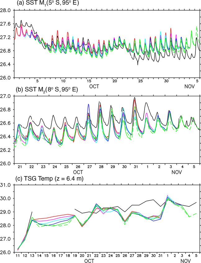
B. Thompson et al.: Coupled forecast model for the Maritime Continent 1085
used to generate the interpolation weights for the remapping
of exchange fields. The coupling occurs at hourly frequency,
and hourly mean fields are exchanged. Since a direct flux
formulation is implemented, the heat fluxes computed using
the Monin–Obukhov similarity theory is exchanged from the
atmosphere to the ocean model. The sea surface tempera-
ture (SST) and zonal and meridional surface current fields
are sent from the ocean to the atmosphere model. The vari-
ables exchanged from atmosphere to the ocean include non-
solar heat flux, net shortwave radiation, liquid precipitation,
net evaporation, and zonal and meridional wind stress. Due
to numerical issues, MSLP exchange from the atmosphere
is not enabled in the MCao . Instead, it is supplied from an
external data source to the ocean model. The MSLP from
ECMWF IFS data have been used in our coupled forecast
simulations.
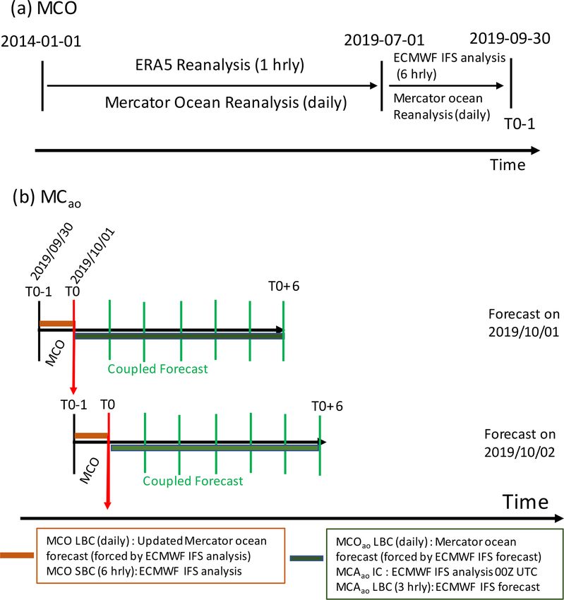
2.5 Model initialisation and forcing
To assess the performance of the ocean model and provide
initial condition to the MCOao , a 69-month hindcast simula-
tion is performed with MCO for the period 1 January 2014
to 30 September 2019. The MCO was initialised in 1 Jan-
Figure 2. Schematic of modelling systems used in the study: (a)
uary 2014 using temperature, salinity, zonal and meridional MC ocean-only model (MCO) hindcast and (b) MC atmosphere–
currents, and SSH derived from Mercator global ocean re- ocean coupled forecast model (MCao ). MCOao stands for the MC
analysis. The lateral boundary condition for the hindcast coupled ocean model, MCAao stand for the MC coupled atmo-
simulation is also obtained from the same ocean reanaly- spheric model, LBC stands for the lateral boundary condition, SBC
sis data. The daily mean of temperature, salinity, baroclinic stands for the surface boundary condition, IC stands for the initial
and barotropic velocities, and SSH are included in the lat- condition.
eral boundary forcing. Ocean surface is forced by ECMWF
Reanalysis 5 (ERA5) during the period from 1 January 2014
to 30 June 2019. Downward shortwave and longwave radi- MCOao , 3-hourly EMCWF IFS forecast data are supplied to
ation at the ocean surface; total precipitation; MSLP; and the model.
10 m wind velocities, air temperature, and specific humid-
ity fields are included in the forcing file. Since there was a 2.6 Pre-operational forecast setup
delay of about 2–3 months in the release of ERA5 data dur-
ing the time of model development, the MCO is forced by The atmosphere–ocean coupled forecast model ran as a pre-
the 6-hourly ECMWF IFS analysis fields from 1 July 2019 operational forecast system from 1 to 31 October 2019 at the
to the start of MCao pre-operational forecast run on 1 Octo- Cray XC-40 HPC located in the Center for Climate Research
ber 2019 (Fig. 2a). As the atmospheric adjustments are sub- Singapore (CCRS), Singapore. The forecast system includes
daily, no spin-up or hindcast simulations are performed for all necessary programs and scripts for the pre-processing of
the MCAao . atmospheric and oceanic variables to their respective model
A schematic of the atmosphere–ocean coupled system grids. The forecast system is scheduled to initialise the fore-
used in the pre-operational forecast is shown in Fig. 2b. In casts daily at 13:00 UTC, and simulations are completed by
the coupled prediction system, the MCAao is initialised daily ∼ 18:40 UTC. Summary of HPC resources usage and typi-
at 00:00 Z UTC from the ECMWF IFS analysis. MCO run for cal runtimes for daily forecast simulations are shown in Ta-
the previous day (T0 minus 1), forced by 6-hourly ECMWF ble 1. To minimise the output size, only basic oceanic and
IFS analysis at the surface and the daily mean of updated atmospheric variables are included in the output. The fore-
Mercator ocean forecast as the LBC, provides the initial con- cast from MCOao includes instantaneous SSH; hourly aver-
dition to MCOao . Since it is driven by analysed (or updated) aged sea surface temperature, sea surface salinity, and sur-
surface (lateral) boundary conditions, the MCO provides an face current velocities; and the daily mean of ocean temper-
updated initial condition to the MCOao daily. The MCao fore- ature, salinity, and ocean currents. Further, to test the fea-
cast run is driven by LBC from 3-hourly ECMWF IFS fore- sibility of the coupled forecast system for operational pur-
casts in the atmosphere and daily Mercator forecasts in the pose, we have conducted simulations with increased compu-
ocean. Since the MSLP from MCAao is not incorporated in tational resources. Test simulations showed that by increas-
https://doi.org/10.5194/gmd-14-1081-2021 Geosci. Model Dev., 14, 1081–1100, 2021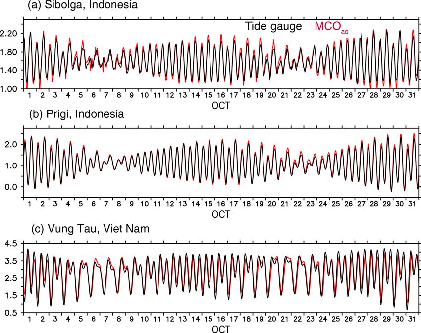
1086                                               B. Thompson et al.: Coupled forecast model for the Maritime Continent

ing the computational resources to 81 nodes (2916 cores), the     improved representer assimilation method. Tidal heights and
total runtime has been reduced to ∼ 140 min. This suggests        currents of 32 tidal constituents are available. The data are
a near-linear reduction in total runtime with an increase in      freely available through http://www.aviso.altimetry.fr/en/
computation nodes.                                                data/products/auxiliary-products/global-tide-fes.html (last
                                                                  access: 25 November 2020).

3     Data                                                        3.2    Model evaluation

                                                                  The CORIOLIS data service provides quality-controlled
A brief description of the reanalysis, forecast, and observa-
                                                                  in situ data in real-time and delayed modes over the
tional datasets used for the model initialisation, forcing, and
                                                                  global ocean. The data include temperature and salinity
evaluation is presented in this section.
                                                                  profiles and time series from profiling floats, expendable
3.1    Model initialisation and forcing                           bathythermographs (XBTs), thermo-salinographs (TSGs),
                                                                  and drifting buoys. The data are freely available from http:
ERA5 is a climate reanalysis produced by the ECMWF                //www.coriolis.eu.org/Data-Products/ (last access: 6 Novem-
providing hourly estimates of many atmospheric, land, and         ber 2020).
oceanic fields (Hersbach et al., 2020). Currently, it covers         The Operational Sea Surface Temperature and Sea Ice
the period from 1979 to within 5 d of the present, and its        Analysis (OSTIA) SST is produced daily on an operational
horizontal resolution is approx. 30 km. The reanalysis is pro-    basis at the UK Met Office using optimal interpolation on
duced using 4D-Var assimilation of the ECMWF Integrated           a global 0.054◦ × 0.054◦ grid. The product assimilates satel-
Forecast System (IFS). ERA5 combines vast amounts of his-         lite data including advanced Very-High Resolution Radiome-
torical observations into global estimates using advanced         ter, Spinning Enhanced Visible and Infrared imager, Geo-
modelling and data assimilation systems. The data are             stationary Operational Environmental Satellite Imager, In-
freely available through the data server https://cds.climate.     frared Atmospheric Sounding Interferometer, and Tropical
copernicus.eu/ (last access: 20 November 2020).                   Rainfall Measuring Mission Microwave imager data and in
   ECMWF IFS is a global weather prediction system com-           situ data from ships and drifting and moored buoys (Don-
prising a spectral atmospheric model, ocean wave model,           lon et al., 2012). SST data at every grid point are accompa-
ocean model, and land surface model coupled to a 4D-              nied by an uncertainty estimate, known as an analysis error,
Var data assimilation system. IFS medium-range weather            and an optimal interpolation approach is employed to pro-
forecasts are available up to 10 d at a horizontal resolu-        duce this estimate. The data are freely available from https:
tion of 0.1◦ . In addition, the atmospheric analysis fields       //marine.copernicus.eu/ (last access: 22 December 2020).
are provided four times daily for the forecast base times            The University of Hawaii Sea Level Center (UHSLC) of-
00:00, 06:00, 12:00, and 18:00 UTC. The data are available        fers quality-controlled tide gauge (TG) sea level observations
to registered users from https://www.ecmwf.int/en/forecasts/      over the global ocean as fast-delivery (FD, 1–2-month de-
datasets/ (last access: 20 November 2019).                        lay) and research-quality (RQ, 1–2-year delay) data at hourly
   Mercator global ocean reanalysis and forecast provides         and daily resolution (Caldwell et al., 2015). The data are
oceanic variables with 0.0833◦ horizontal resolution (Lel-        freely available from http://uhslc.soest.hawaii.edu/data/ (last
louche et al., 2018). The system uses NEMO v3.1 with 50           access: 23 November 2020).
vertical z levels ranging from zero to 5500 m and forced by
the ECMWF IFS meteorological variables. The assimilation          4     Results and discussion
and forecast product includes the daily mean of tempera-
ture, salinity, currents from top to bottom over the global       An evaluation of the MCO hindcast and MCOao forecast sim-
ocean, and SSH. The data are freely available from https:         ulations are presented in this section of the paper. Direct
//marine.copernicus.eu/ (last access: 20 December 2020).          comparison of model simulations with observation or anal-
   The tidal heights and currents computed from the global        ysis data has been performed. Based on the availability of
tide model finite-element solution (FES2014b) is used as          in situ or satellite observation at the time of data analysis,
the tidal forcing in the model. FES2014 is based on the           only a few variables are selected for assessing the model per-
resolution of the shallow water hydrodynamic equations            formance. In addition, to maintain consistency between the
(T-UGO model) in a spectral configuration and using a             evaluation of hindcast and forecast simulations, analyses of
global finite-element mesh with increasing resolution in          the same set of variables and observation data have been per-
coastal and shallow waters regions (Lyard et al., 2006).          formed where possible. Oceanic variables employed for the
The database is distributed on a global 0.0625◦ × 0.0625◦         evaluation are SST, SSH, and the subsurface temperature and
grid. Data are produced by assimilating long-term altimetry       salinity.
data (Topex, Poseidon, Jason-1, Jason-2, TPN-J1N, and
ERS-1, ERS-2, ENVISAT) and tidal gauges through an

Geosci. Model Dev., 14, 1081–1100, 2021                                            https://doi.org/10.5194/gmd-14-1081-2021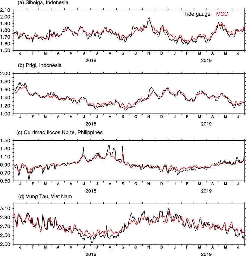
B. Thompson et al.: Coupled forecast model for the Maritime Continent 1087
Table 1. Summary of HPC resources usage and typical runtimes.
Configuration Uncoupled ocean Coupled atmosphere Coupled ocean
(MCO) (MCAao ) (MCOao )
Total nodes (cores) 16 (576) 24 (864) 4 (144)
Daily runtime 6.5 min 330 min
Core hours 3.9 198
Flume/IO (node) 1
4.1 Ocean hindcast
An overall assessment of the ocean model hindcast simu-
lation is carried out to understand the realism of the ocean
initial condition for the coupled forecasts, particularly at the
ocean surface where the exchange of fluxes between the at-
mosphere and ocean takes place. Though the hindcast sim-
ulations encompass from 1 January 2014 to 30 Septem-
ber 2019, we only evaluate ERA5-driven simulations dur-
ing the period from 1 January 2018 to 30 June 2019. The
first 4 years of the simulation data are considered the spin-
up stage of the model. Comparison of daily mean SST with
OSTIA analysis and moored buoys observations is presented,
while the daily mean SSH is compared with tide gauge obser-
Figure 3. Domain used for hindcast and forecast evaluation with
vations. Moored observation buoys in the eastern tropical In-
sub-regions defined in the study: (1) Andaman Sea–Malacca Strait
dian Ocean established as part of the Research Moored Array
(ASMS), (2) southern South China Sea (SSCS), (3) Gulf of Thai-
land (GoT), (4) the rest of the South China Sea (RSCS), (5) the for African–Asian–Australian Monsoon Analysis (RAMA,
tropical western Pacific Ocean (TWPO), (6) Sulu–Celebes seas McPhaden et al., 2009) at the locations 5◦ S, 95◦ E (M1 ) and
(SuCeS), (7) Banda Sea (BS), (8) Java Sea (JS), (9) Timor–Arafura 8◦ S, 95◦ E (M2 ) are used for the evaluation. Fast-delivery
seas (TAS), and (10) the tropical eastern Indian Ocean (TEIO). The (FD) data from UHSLC for 20 tide gauge stations are em-
Bay of Bengal region (north of 5◦ N, west of 92◦ E) is excluded ployed for the SSH comparison.
when analysis is performed for different sub-regions. The blue line
in the TAS indicates the TSG observation track. The locations of 4.1.1 Sea surface temperature
tide gauges are shown as black circles. Moored buoy locations M1
(5◦ S, 95◦ E) and M2 ( 8◦ S, 95◦ E) are also shown. Comparison of model-simulated daily mean SST with OS-
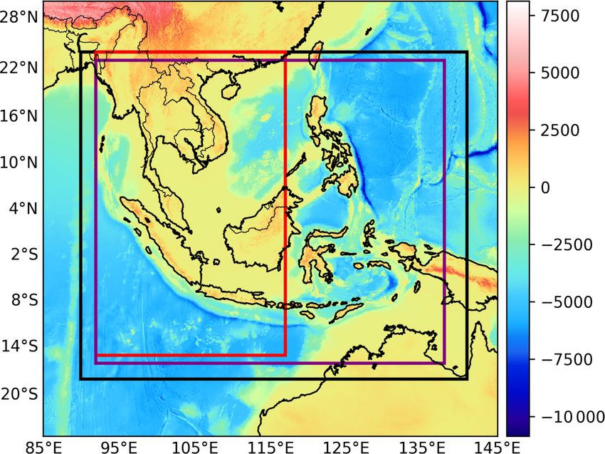
TIA analysis is shown in Fig. 4. Spatial distribution of model
SST bias (Fig. 4a), root-mean-square difference (RMSD)
Model hindcasts and forecasts over the region 16◦ S to (Fig. 4b), correlation coefficient (Fig. 4c) and the spatial av-
23◦ N and 92 to 138◦ E and defined as the analysis domain erage of SST difference over the analysis domain (Fig. 4d)
(Figs. 1 and 3), is further used for the analysis. The MC are given. Model performance in simulating SST over the
model domain includes oceanic basins with different geo- sub-regions is given in Table 2. SST Bias, RMSD, and
graphical and climatological characteristics. For the evalu- correlation coefficient statistics computed using modelled
ation purpose, we have divided the analysis-domain into 10 SST and OSTIA are shown in Table 2. The SST bias is
sub-regions based on their geographical distribution (Fig. 3). within ±0.2 ◦ C for about 76 % of the analysis domain and
These sub-regions are the (1) Andaman Sea–Malacca Strait within ±0.5 ◦ C for about 98 % of the analysis domain. The
(ASMS), (2) southern South China Sea (SSCS), (3) Gulf of largest SST cold bias is seen in the Andaman Sea region.
Thailand (GoT), (4) the rest of the South China Sea (RSCS), Meanwhile, most of the South China Sea (SCS), equato-
(5) the tropical western Pacific Ocean (TWPO), (6) Sulu– rial western Pacific Ocean, and the Australian coast of the
Celebes seas (SuCeS), (7) Banda Sea (BS), (8) Java Sea (JS), Timor Sea show a positive SST bias. Negative SST bias of
(9) Timor–Arafura seas (TAS), and (10) the tropical eastern about −0.25 ◦ C is observed in the ASMS region, while pos-
Indian Ocean (TEIO). itive bias over 0.25 ◦ C is confined to the SSCS and GoT
sub-regions. Rather than appearing as a basin-wide feature,
higher positive biases appear as small circular patches in the
northern SCS region that represent the likely existence of cy-
clonic eddies over this region.
https://doi.org/10.5194/gmd-14-1081-2021 Geosci. Model Dev., 14, 1081–1100, 2021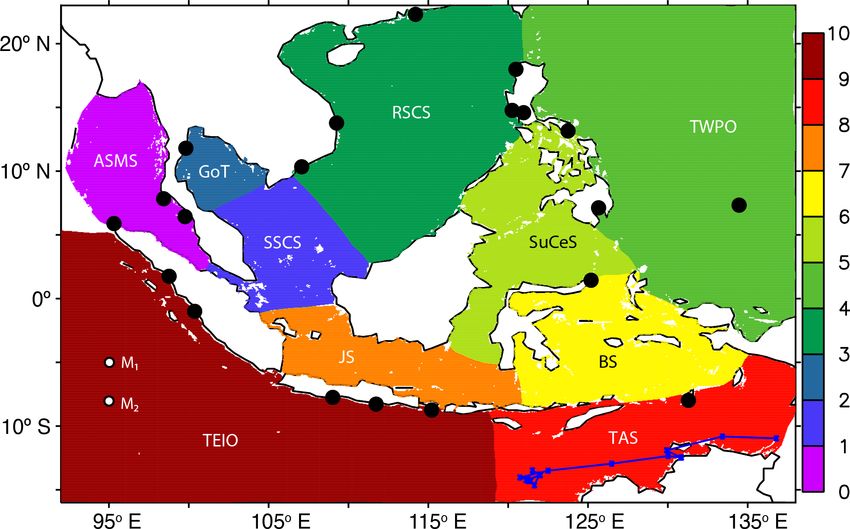
1088                                                   B. Thompson et al.: Coupled forecast model for the Maritime Continent

Figure 4. Spatial distribution of daily averaged (a) SST bias (◦ C), (b) RMSD (◦ C), and (c) correlation coefficient between the MCO hindcast
and OSTIA analysis. (d) Spatial average of SST difference between the model and OSTIA over the analysis domain (◦ C).

   The RMSD between the model and OSTIA is less than                     2019 and September–October in 2018 (figures not shown).
0.5 ◦ C for about 97 % of the analysis domain (Fig. 4b).                 Meanwhile, SST simulation over those sub-regions shows
Small patches of higher RMSD (> 0.7 ◦ C) are mostly seen                 improvement during June–July 2018. Higher negative SST
along the coastal regions. The RMSD minimum (0.25 ◦ C)                   bias over the ASMS region mainly contributes to the negative
and maximum (0.53 ◦ C) are observed over the BS and ASMS                 SST difference during the same period. Overall, the mean
sub-regions, respectively (Table 2). Correlation between the             SST bias, RMSD, and mean correlation over the analysis do-
model SST hindcast and OSTIA is above 99.9 % confi-                      main are 0.07 ◦ C, 0.34 ◦ C, and 0.90, respectively.
dence level over the analysis domain (Fig. 4c). Over 88 %                   The time series of daily mean SST from the RAMA
of the domain displays a correlation higher than 0.8. Rela-              moored observation buoys located in the southeastern trop-
tively low correlation is seen over the middle of the Malacca            ical Indian Ocean at 5◦ S, 95◦ E (M1 ) and 8◦ S, 95◦ E (M2 )
Strait, Makassar Strait, and equatorial Pacific Ocean regions.           is shown in Fig. 5. Model SST is bilinearly interpolated to
In sub-region spatial average, the lowest (0.8) and highest              the buoy locations. Temperature observations at 1 m depth
(0.96) correlations are seen over the SuCeS and RSCS re-                 are taken as SST from the moored buoys, while temperature
gions, respectively (Table 2). Time series of the spatially              averaged over the upper 1 m is indicated as the model SST
averaged SST difference between the model and OSTIA is                   at these locations. In general, a good agreement is found be-
shown in Fig. 4d. Consistent with our earlier analyses, rela-            tween the model and observations at both mooring locations.
tively low SST difference depicts a good agreement between               Both the seasonal and intra-seasonal SST variability are rea-
the MCO SST hindcast and OSTIA analysis. Further analysis                sonably well reproduced by the model. SST bias, RMSD, and
of SST in different sub-regions revealed that relatively higher          correlation between the model and observation are 0.17 ◦ C,
SST over the GoT, SSCS and SuCeS regions contribute to the               0.29 ◦ C, and 0.94, respectively, for M1 and 0.12 ◦ C, 0.41 ◦ C,
positive SST differences during February–April in 2018 and               and 0.92, respectively, for M2 . The standard deviation (SD)

Geosci. Model Dev., 14, 1081–1100, 2021                                                    https://doi.org/10.5194/gmd-14-1081-2021
B. Thompson et al.: Coupled forecast model for the Maritime Continent                                                            1089

Table 2. Summary of SST bias, RMSD, and correlation coefficient statistics between the model hindcast and OSTIA for the period 1 Jan-
uary 2018 to 30 June 2019. Daily mean SST from the model and OSTIA is used for the analysis.

                               No.    Region                                Bias    RMSD       Correlation
                                                                            (◦ C)    (◦ C)     Coefficient
                               1     Andaman Sea–Malacca Strait         −0.25         0.53           0.84
                               2     Southern SCS                        0.29         0.30           0.95
                               3     Gulf of Thailand                    0.26         0.30           0.94
                               4     Rest of SCS                         0.16         0.39           0.96
                               5     Tropical western Pacific Ocean      0.07         0.29           0.88
                               6     Sulu–Celebes seas                   0.12         0.31           0.80
                               7     Banda Sea                           0.00         0.25           0.84
                               8     Java Sea                            0.09         0.30           0.89
                               9     Timor–Arafura seas                  0.01         0.34           0.95
                               10    Tropical eastern Indian Ocean      −0.05         0.30           0.92
                               Mean value                                0.07         0.34           0.90

                                                                      bias, RMSD, and mean correlation between the model and
                                                                      observation are 0.01 m, 0.06 m, and 0.87, respectively.
                                                                         Time series of daily mean SSH from model and observa-
                                                                      tions for randomly selected stations are plotted in Fig. 6. The
                                                                      stations Sibolga and Prigi are located in the eastern tropical
                                                                      Indian Ocean, and Currimao Ilocos Norte and Vung Tau are
                                                                      located in the SCS. Generally, the model-simulated SSH fol-
                                                                      lows the observation and shows good agreement with it. A
                                                                      few sharp peaks in the tide gauge observation are found to
                                                                      be absent in the model simulation (e.g. Fig. 6c). Most of the
                                                                      tide gauge stations are located adjacent to the coast, and our
                                                                      current model resolution is not enough to resolve the coast-
Figure 5. Comparison of daily averaged SST from MCO hindcast
and RAMA moored buoys at (a) M1 and (b) M2 during the period          line at very fine scales. Since the model SSH is interpolated
1 January 2018 to 30 June 2019.                                       to the tide gauge location, local-scale SSH variations may
                                                                      not be captured in the model simulation. This may be one
                                                                      possible reason for the discrepancy between the model and
                                                                      observations.
of SST at M1 and M2 are 0.94 ◦ C and 0.99 ◦ C, respectively,             Comparison of model-simulated SST and SSH fields
and the RMSD is smaller than the SD at both locations.                shows good agreement with observation and analysis data.
                                                                      The RMSD and bias statistics of SST and SSH relative to the
4.1.2   Sea surface height                                            observation are within the acceptable error limits of ocean
                                                                      hindcast simulations (e.g. Yang et al., 2016). Statistically sig-
Daily mean SSH observation from 20 tide-gauge stations dis-           nificant correlation with observation suggests that both the
tributed across the domain and MCO simulated SSH interpo-             spatial and temporal patterns of variability are reasonably
lated to the location of these observations have been used            well reproduced by the model.
for the hindcast evaluation. SSH bias, RMSD and correlation
coefficient statistics between model and SSH observations             4.2     Ocean forecasts
are given in Table 3. Highest SSH bias (0.12 m) and RMSD
(0.15 m) are seen at the Malakal, Palau, tide gauge station.          Results from the analysis of MCOao forecast simulations for
The SSH bias is within ±0.05 m for 17 of the total 20 sta-            October 2020 are presented here. Since the system delivers
tions analysed. The model accuracy is higher than 0.10 m for          a 6 d forecast, the analysis period extends from 1 October to
18 stations, while 14 of the total 20 stations have an accuracy       5 November 2020. Daily files are produced at different fore-
greater than 0.05 m. The SSH correlation between the model            cast lead times, T +0 to T +24 (fcst_day1), T +24 to T +48
and observations is above 99.9 % confidence level for all tide        (fcst_day2), T +48 to T +72 (fcst_day3), T +72 to T +96
gauge stations employed in the analysis. The correlation is           (fcst_day4), T +96 to T +120 (fcst_day5), and T +120 to
above 0.80 for 16 tide gauge stations. Lowest correlation of          T +144 (fcst_day6) for the following analyses. Comparisons
0.60 is observed at the Malakal tide gauge station. Mean SSH          of coupled ocean forecasts for different forecast lead times

https://doi.org/10.5194/gmd-14-1081-2021                                                     Geosci. Model Dev., 14, 1081–1100, 2021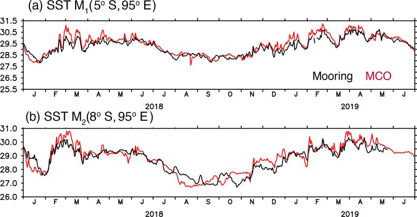
1090                                                B. Thompson et al.: Coupled forecast model for the Maritime Continent

Table 3. Summary of SSH bias, RMSD, and correlation coefficient statistics between MCO hindcast and tide gauge stations for the period
1 January 2018 to 30 June 2019. Daily mean SSH from model and tide gauge is used for the analysis.

                 No     Station name and                    Latitude,                  Bias    RMSD      Correlation
                        country                             longitude                  (m)       (m)      coefficient
                 1    Sabang, Indonesia                     5.888◦ N, 95.317◦ E       0.00       0.04           0.85
                 2    Sibolga, Indonesia                    1.75◦ N, 98.767◦ E        0.01       0.03           0.90
                 3    Padang, Indonesia                     1.0◦ S, 100.367◦ E       −0.05       0.06           0.89
                 4    Cilicap, Indonesia                    7.752◦ S, 109.017◦ E      0.00       0.04           0.93
                 5    Prigi, Indonesia                      8.28◦ S, 111.73◦ E        0.00       0.05           0.96
                 6    Benoa, Indonesia                      8.745◦ S, 115.21◦ E       0.00       0.04           0.94
                 7    Saumlaki, Indonesia                   7.982◦ S, 131.29◦ E       0.02       0.05           0.81
                 8    Bitung, Indonesia                     1.44◦ N, 125.193◦ E       0.06       0.07           0.73
                 9    Malakal, Palau                        7.33◦ N, 134.463◦ E       0.12       0.15           0.60
                 10   Davao Gulf, Philippines               7.122◦ N, 125.663◦ E      0.00       0.03           0.88
                 11   Subic Bay, Philippines                14.765◦ N, 120.252◦ E     0.04       0.05           0.94
                 12   Manila, Philippines                   14.585◦ N, 120.968◦ E    −0.01       0.04           0.95
                 13   Legaspi, Philippines                  13.15◦ N, 123.75◦ E       0.00       0.03           0.83
                 14   Currimao Ilocos Norte, Philippines    17.988◦ N, 120.488◦ E     0.00       0.05           0.96
                 15   Hong Kong, China                      22.3◦ N, 114.2◦ E        −0.02       0.09           0.75
                 16   Qui Nhon, Viet Nam                    13.775◦ N, 109.255◦ E     0.01       0.05           0.90
                 17   Vung Tau, Viet Nam                    10.34◦ N, 107.072◦ E      0.01       0.07           0.90
                 18   Ko Lak, Thailand                      11.795◦ N, 99.817◦ E     −0.01       0.06           0.95
                 19   Ko Taphao Noi, Thailand               7.832◦ N, 98.425◦ E       0.00       0.04           0.91
                 20   Pulau Langkawi, Malaysia              6.432◦ N, 99.765◦ E      −0.03       0.14           0.72
                 Mean values                                                          0.01       0.06           0.87

with OSTIA SST and in situ observations have been per-               series considerably decreases with higher forecast lead times
formed, such as temperature from RAMA moored buoys,                  (Table 4).
TSG, and XBT profiles; temperature and salinity from con-               SST correlation is above the 95 % confidence level
ductivity temperature depth (CTD) profiles; and SSH from             (r > 0.365) over the entire analysis domain during fcst_day1.
tide gauges.                                                         In general, SST correlation is higher than 99 % confi-
                                                                     dence level (r > 0.46) over 60 % of the sub-regions during
4.2.1   Sea surface temperature                                      higher forecast lead times as well. The sub-regions includ-
                                                                     ing ASMS, GoT, TWPO, and SuCeS are noted by lower cor-
Time series of daily mean SST averaged over the sub-regions          relation significance level with an increase in forecast lead
from OSTIA analysis and different forecast lead times are            time. Overall, the SST correlation over the analysis domain
plotted in Fig. 7. Statistics of SST bias, RMSD, and corre-          is above the 99 % confidence level across all forecast lead
lation coefficient between the model and OSTIA for the Oc-           times, while bias and RMSD are less than 0.19 and 0.35 ◦ C,
tober forecast run are listed in Table 4. The forecasted SST         respectively.
over most of the sub-regions is within the error standard de-           Figure 8 shows the time series of hourly averaged SST at
viation of the OSTIA analysis, which is indicated by shad-           M1 (Fig. 8a) and M2 (Fig. 8b) mooring locations from ob-
ing in Fig. 7. Excluding the ASMS, all other sub-regions             servation and model forecasts. It should be noted that the
exhibit a warm SST bias, with the largest values over the            observation at M2 is available for a relatively short period
SSCS and GoT. The RMSD is less than 0.5 ◦ C over most of             from 21 October to 5 November 2020. Statistics of the SST
the sub-regions during the analysis period. Over the ASMS            bias, RMSD, and correlation coefficient between the model
sub-region, both the cold bias and RMSD increase with the            forecast and the observations are listed in Table 5. The diur-
forecast lead time, and it shows the highest RMSD (0.49 ◦ C)         nal variability of SST at both locations is reasonably well
on fsct_day6. The largest SST RMSD (0.56 ◦ C) and bias               reproduced by the model in all forecast lead times. How-
(0.49 ◦ C) over all sub-regions is observed over the GoT with        ever, the model forecasts have overestimated the SST diurnal
a 1 d forecast lead time. Generally, the forecasted SST tends        variations from 23 October 2019. SST cooling during late
to be cooler, with an increase in forecast lead time denoting        October–early August 2020 at the location M1 is underesti-
a lower warm bias and RMSD relative to fcst_day1. Inter-             mated in the model forecast. SST bias and RMSD at M1 are
estingly, inconsistent with the improvements in SST bias and         less than 0.07 and 0.20 ◦ C, respectively, and remain fairly
RMSD, the correlation between forecasted and OSTIA time              constant across all forecast lead times. Despite this, the cor-

Geosci. Model Dev., 14, 1081–1100, 2021                                               https://doi.org/10.5194/gmd-14-1081-2021
B. Thompson et al.: Coupled forecast model for the Maritime Continent 1091
Figure 6. Time series of daily mean SSH (in metres) from tide gauge observations (black line) and MCO hindcasts (red line) at randomly
selected stations, (a) Sibolga (1.75◦ N, 98.76◦ E), (b) Prigi (8.28◦ S, 111.73◦ N), (c) Currimao Ilocos Norte (17.988◦ N, 120.488◦ E), and
(d) Vung Tau (10.34◦ N, 107.072◦ E), from 1 January 2018 to 30 June 2019.
relation between model forecasts and observations depicts a cast system produces only daily averaged subsurface vari-
considerable decrease at higher forecast lead times. A cold ables. Hence, the instantaneous TSG temperature observa-
SST bias of about −0.14 to −0.17 ◦ C is noted at location tions at 12:00 UTC are compared with the daily averaged
M2 . The RMSD at M2 is relatively low, with a maximum of model temperature. Time series of TSG temperature obser-
0.18 ◦ C across all forecast lead times while compared to M1 . vations and model forecasts for different forecast lead times
The SST correlation at M2 is above the 95 % confidence level are shown in Fig. 8c. Though the model temperature shows a
(r > 0.61, df ≥ 9) during all forecast lead times. negative bias, daily temperature variation is reasonably well
predicted by the model. This is supported by the high corre-
4.2.2 Temperature and salinity lation, above the 99.9 % confidence level, between the model
forecast and observation (Table 5, item 3). The largest tem-
Temperature and salinity data available from the CORIO- perature bias and RMSD are −0.47 ◦ C and 0.68 ◦ C, respec-
LIS data portal are employed for the MCOao forecast eval- tively, and significant variations in bias, RMSD, and correla-
uation of subsurface fields. Argo and XBT profiles, moored tion statistics are not noticeable.
buoys, and TSG observations are used for the analysis. We The moored buoy observations provide a unique oppor-
only consider mooring and TSG observations with a min- tunity to assess the model simulations both in the surface
imum of 10 d for the analysis. TSG observation selected and subsurface of the ocean. Since the variables of interest
for the analysis is located in the Timor and Arafura seas, in the present study are temperature and salinity, we have
and the track has a direction of motion towards the west tried to compare the model forecast of temperature and salin-
(Fig. 3). Continuous observations available at 6.4 m depth ity with buoy observation available at the locations M1 and
are compared with the model forecasts. Currently, the fore-
https://doi.org/10.5194/gmd-14-1081-2021 Geosci. Model Dev., 14, 1081–1100, 20211092 B. Thompson et al.: Coupled forecast model for the Maritime Continent
Table 4. Summary of SST bias and RMSD (a) and correlation coefficient (b) statistics between coupled ocean forecasts and OSTIA over the
sub-regions shown in Fig. 3 from 1 to 31 October 2019. Daily mean SST from model and OSTIA is used for the analysis.
(a) No. Bias (◦ C) RMSD (◦ C)
Forecast lead time (d) Forecast lead time (d)
1 2 3 4 5 6 1 2 3 4 5 6
1 Andaman Sea–Malacca Strait −0.01 −0.11 −0.13 −0.14 −0.15 −0.17 0.40 0.41 0.41 0.43 0.46 0.49
2 Southern SCS 0.43 0.32 0.27 0.20 0.20 0.20 0.50 0.41 0.36 0.30 0.30 0.30
3 Gulf of Thailand 0.49 0.38 0.29 0.28 0.25 0.23 0.56 0.47 0.37 0.38 0.34 0.33
4 Rest of SCS 0.16 0.10 0.08 0.07 0.05 0.05 0.30 0.24 0.22 0.21 0.20 0.21
5 Tropical western Pacific Ocean 0.11 0.11 0.10 0.09 0.08 0.07 0.21 0.22 0.21 0.20 0.20 0.21
6 Sulu–Celebes seas 0.21 0.14 0.13 0.11 0.10 0.10 0.33 0.27 0.27 0.26 0.26 0.26
7 Banda Sea 0.13 0.10 0.10 0.10 0.10 0.11 0.21 0.19 0.19 0.19 0.21 0.23
8 Java Sea 0.15 0.10 0.09 0.07 0.06 0.05 0.25 0.21 0.21 0.20 0.19 0.19
9 Timor–Arafura seas 0.18 0.17 0.17 0.17 0.17 0.17 0.34 0.34 0.34 0.34 0.35 0.37
10 Tropical eastern Indian Ocean 0.02 0.02 0.02 0.02 0.01 0.01 0.25 0.23 0.22 0.22 0.22 0.22
Mean values 0.19 0.13 0.11 0.10 0.09 0.08 0.35 0.31 0.29 0.28 0.29 0.29
0.12 0.30
(b) No. Correlation coefficient
Forecast lead time (d)
1 2 3 4 5 6
1 Andaman Sea–Malacca Strait 0.37 0.37 0.31 0.23 0.16 0.15
2 Southern SCS 0.63 0.50 0.52 0.53 0.51 0.49
3 Gulf of Thailand 0.48 0.41 0.38 0.33 0.30 0.37
4 Rest of SCS 0.65 0.63 0.62 0.63 0.62 0.61
5 Tropical western Pacific Ocean 0.58 0.49 0.45 0.39 0.34 0.30
6 Sulu–Celebes seas 0.40 0.35 0.30 0.27 0.25 0.24
7 Banda Sea 0.84 0.82 0.83 0.80 0.77 0.72
8 Java Sea 0.88 0.88 0.87 0.87 0.86 0.85
9 Timor–Arafura seas 0.83 0.84 0.84 0.82 0.79 0.76
10 Tropical eastern Indian Ocean 0.53 0.54 0.53 0.52 0.50 0.47
Mean value 0.62 0.58 0.57 0.54 0.51 0.50
0.55
Table 5. Items (1) and (2) are a summary of SST bias and RMSD (a) and correlation coefficient (b) statistics between coupled ocean forecasts
and observations at the mooring locations M1 (5◦ S, 95◦ E) and M2 (8◦ S, 95◦ E) during October 2019. Hourly averaged temperature from
the model and observations is used for the analysis. Item (3) is the same as items (1) and (2) but for temperatures at 6.4 m depth along the
track shown in Fig. 3. Daily averaged temperature from model and instantaneous temperature at 12:00 UTC from observation is used for the
analysis. Item (4) is the same as items (1) and (2) but for temperatures within 0 to 600 m depth at the mooring location M1 . Daily averaged
temperature model and observations used in the analysis.
(a) No. Bias (◦ C) RMSD (◦ C)
Forecast lead time (d) Forecast lead time (d)
1 2 3 4 5 6 1 2 3 4 5 6
(1) SST M1 (5◦ S, 95◦ E) 0.07 0.06 0.06 0.06 0.06 0.06 0.19 0.19 0.19 0.18 0.20 0.20
(2) SST M2 (8◦ S, 95◦ E) −0.14 −0.17 −0.17 −0.15 −0.15 −0.16 0.15 0.18 0.18 0.17 0.17 0.18
(3) Temp (TSG, z = 6.4 m) −0.47 −0.43 −0.43 −0.43 −0.41 −0.46 −0.65 0.65 0.66 0.68 0.64 0.64
(4) Temp M1 (z = 0–600 m, 5◦ S, 95◦ E) 1.87 1.87 1.88 1.91 1.91 1.95 2.83 2.82 2.83 2.88 2.89 2.96
(b) No. Correlation coefficient
Forecast lead time (d)
1 2 3 4 5 6
(1) SST M1 (5◦ S, 95◦ E) 0.77 0.74 0.61 0.54 0.34 0.24
(2) SST M2 (8◦ S, 95◦ E) 0.94 0.91 0.83 0.79 0.78 0.68
(3) Temp (TSG, z = 6.4 m) 0.87 0.86 0.85 0.83 0.84 0.86
(4) Temp M1 (z = 0–600 m, 5◦ S, 95◦ E) 0.60 0.61 0.58 0.55 0.52 0.56
Geosci. Model Dev., 14, 1081–1100, 2021 https://doi.org/10.5194/gmd-14-1081-2021B. Thompson et al.: Coupled forecast model for the Maritime Continent 1093 Figure 7. Time series of daily mean SST from model forecast and OSTIA averaged over the sub-regions: OSTIA (black line), fcst_day1 (red line), fcst_day2 (purple line), fcst_day3 (light blue line), fcst_day4 (blue line), fcst_day5 (green line), and fcst_day6 (dashed green line). Shading represents the estimated error standard deviation of analysed SST in OSTIA. (a) ASMS stands for Andaman Sea–Malacca Strait, (b) SSCS stands for southern SCS, (c) GoT stands for Gulf of Thailand, (d) RSCS represents the rest of the SCS, (e) TWPO stands for tropical western Pacific Ocean, (f) SuCeS stands for the Sulu–Celebes seas, (g) BS stands for the Banda Sea, (h) JS stands for the Java Sea, (i) TAS stands for the Timor–Arafura seas, (j) TEIO stands for tropical eastern Indian Ocean. The y axes are differ between the plots. M2 . However, due to data gaps and shorter time series, salin- shoaling in late October are well simulated by the model. ity observation from both moorings and temperature from A significant difference between the model forecast and ob- M2 mooring are not included in the analysis. Depth–time servations is seen in the region below the mixed layer. The plots of temperature from the model for forecast lead times model simulation is unable to reproduce the sharp temper- 1 d (fcst_day1), 3 d (fcst_day3), and 5 d (fcst_day5) and the ature stratification and cooling in the thermocline regions, moored observation (M1 ) are shown in Fig. 9. Statistics of while this feature is clearly evident in the observations. This temperature bias, RMSD, and correlation coefficient between leads to a relatively large discrepancy between the model and the model forecast and observations are given in Table 5. The observation in the subsurface region roughly between 100 depth of the upper ocean isothermal and mixed layer and its to 250 m depths. The usage of daily averaged temperature https://doi.org/10.5194/gmd-14-1081-2021 Geosci. Model Dev., 14, 1081–1100, 2021
1094                                                        B. Thompson et al.: Coupled forecast model for the Maritime Continent

Table 6. Summary of temperature and salinity RMSD statistics between coupled ocean forecasts and in situ (Argo profile and XBT) obser-
vations from 1 October to 5 November 2019. Daily averaged temperature from the model and instantaneous temperature or salinity from
observations are used for the analysis. Numbers in bold indicate the number of profiles analysed for each variable and lead forecast time.

                                                                                           RMSD
                                                                      Forecast lead time (d)                       All forecasts
                                                            1         2        3           4          5        6
                                  Temperature (◦ C)     1.40        1.41    1.40     1.41        1.41     1.41              1.41
                                  278                    255        251      250      246        245       245
                                  Salinity (psu)        0.14        0.14    0.14     0.14        0.15     0.14              0.14
                                  244                    226         223     222      217         216      216

Table 7. Summary of SSH RMSD and bias statistics between coupled ocean forecasts and tide gauge observations during October 2019.
Hourly instantaneous SSH from the model and observations is used for the analysis.

 No.   Station name &               Latitude,                                 RMSD                                                   Bias
       country                      longitude                                  (m)                                                   (m)
                                                                      Forecast lead time (days)                            Forecast lead time (days)
                                                                1      2       3       4         5        6        1       2        3         4        5       6
 1     Sabang, Indonesia            5.888◦ N, 95.317◦ E     0.06     0.06   0.06    0.06       0.06   0.07      0.01    0.01    0.01      0.01     0.02     0.02
 2     Sibolga, Indonesia           1.75◦ N, 98.767◦ E      0.07     0.06   0.06    0.07       0.07   0.08      0.01    0.02    0.03      0.04     0.04     0.05
 3     Padang, Indonesia            1.0◦ S, 100.367◦ E      0.05     0.05   0.05    0.05       0.05   0.05      0.00    0.00    0.00      0.00     0.00     0.00
 4     Cilicap, Indonesia           7.752◦ S, 109.017◦ E    0.09     0.08   0.08    0.08       0.08   0.08      0.04    0.04    0.04      0.04     0.04     0.04
 5     Prigi, Indonesia             8.28◦ S, 111.73◦ E      0.10     0.10   0.11    0.11       0.11   0.11      0.05    0.05    0.06      0.06     0.06     0.07
 6     Benoa, Indonesia             8.745◦ S, 115.21◦ E     0.11     0.10   0.10    0.10       0.10   0.10     −0.03   −0.03   −0.02     −0.02    −0.02    −0.02
 7     Saumlaki, Indonesia          7.982◦ S, 131.29◦ E     0.10     0.10   0.10    0.10       0.11   0.11      0.05    0.05    0.05      0.06     0.06     0.06
 8     Bitung, Indonesia            1.44◦ N, 125.193◦ E     0.10     0.10   0.10    0.10       0.10   0.10      0.08    0.08    0.08      0.08     0.08     0.08
 9     Malakal, Palau               7.33◦ N, 134.463◦ E     0.07     0.07   0.07    0.07       0.07   0.07      0.01    0.01    0.01      0.01     0.01     0.01
 10    Davao Gulf, Philippines      7.122◦ N, 125.663◦ E    0.08     0.09   0.09    0.09       0.09   0.09     −0.03   −0.03   −0.02     −0.02    −0.02    −0.01
 11    Subic Bay, Philippines       14.765◦ N, 120.252◦ E   0.04     0.04   0.04    0.03       0.03   0.03      0.00    0.00    0.00      0.00     0.00     0.00
 12    Manila, Philippines          14.585◦ N, 120.968◦ E   0.08     0.08   0.07    0.07       0.07   0.07     −0.04   −0.04   −0.04     −0.04    −0.04    −0.04
 13    Legaspi, Philippines         13.15◦ N, 123.75◦ E     0.06     0.06   0.06    0.06       0.06   0.06      0.01    0.01    0.01      0.01     0.01     0.01
 14    Hong Kong, China             22.3◦ N, 114.2◦ E       0.18     0.18   0.18    0.18       0.18   0.18     −0.08   −0.09   −0.09     −0.09    −0.10    −0.10
 15    Qui Nhon, Viet Nam           13.775◦ N, 109.255◦ E   0.08     0.08   0.08    0.08       0.08   0.08     −0.02   −0.02   −0.02     −0.03    −0.03    −0.03
 16    Vung Tau, Viet Nam           10.34◦ N, 107.072◦ E    0.33     0.33   0.32    0.33       0.32   0.32      0.00    0.00   −0.01     −0.01    −0.02    −0.02
 17    Ko Lak, Thailand             11.795◦ N, 99.817◦ E    0.17     0.16   0.16    0.19       0.18   0.19     −0.03   −0.02   −0.04     −0.07    −0.07    −0.08
 18    Ko Taphao Noi, Thailand      7.832◦ N, 98.425◦ E     0.17     0.17   0.17    0.17       0.17   0.17      0.00    0.00    0.00      0.00     0.00     0.01
 19    Pulau Langkawi, Malaysia     6.432◦ N, 99.765◦ E     0.29     0.27   0.27    0.26       0.26   0.25     −0.05   −0.04   −0.03     −0.03    −0.03    −0.02
 Mean values                                                0.14     0.14   0.14    0.14       0.14   0.14      0.00    0.00    0.00      0.00     0.00     0.00

rather than instantaneous profile or higher vertical mixing in                     November 2020), the analysis mainly demonstrates the
the model may be one of the possible reasons for this dis-                         model performance in the domain excluding the SCS region.
crepancy. Larger temperature differences at the thermocline                        As observed in the M1 mooring location, warm biases with
region have led to a warm temperature bias in the model                            varying magnitude are seen in the thermocline region across
forecast (Table 5). Maximum temperature bias and RMSD                              the analysis domain (figures not shown). Considering the
are 1.95 and 2.96 ◦ C, respectively. Meanwhile, the correla-                       depth range where this bias exists, the vertical mixing param-
tion between the model forecast and observation is above                           eterisation may have a stronger influence in modifying the
the 99 % confidence level (r > 0.47) across all forecast lead                      thermal stratification than the penetrative shortwave forcing.
times.                                                                             Statistics of RMSD for ocean temperature and salinity rela-
   Argo and XBT profiles available for the period 1 Oc-                            tive to all profile observations are given in Table 6. RMSD of
tober to 5 November 2019 are compared with the model                               individual profiles are first computed and then a root-mean-
forecast to derive the RMSD statistics for temperature                             square (rms) value of the computed RMSD is derived. RMSD
and salinity. Since no temperature or salinity profiles                            across all forecast lead times and with the number of pro-
are available in the SCS (figure not shown, data dis-                              files analysed are listed. For both temperature and salinity,
tribution can be viewed from http://www.coriolis.eu.org/                           the RMSD remains fairly similar during the entire analysis
Data-Products/Data-Delivery/Data-selection, last access: 6                         period. Over the analysis domain and across all forecast lead

Geosci. Model Dev., 14, 1081–1100, 2021                                                                       https://doi.org/10.5194/gmd-14-1081-2021
You can also read