Estimation of the non-exceedance probability of extreme storm surges in South Korea using tidal-gauge data
←
→
Page content transcription
If your browser does not render page correctly, please read the page content below
Nat. Hazards Earth Syst. Sci., 2121, 2611–2631, 20212021
https://doi.org/10.5194/nhess-2121-2611-20212021
© Author(s) 2021. This work is distributed under
the Creative Commons Attribution 4.0 License.

Estimation of the non-exceedance probability of extreme
storm surges in South Korea using tidal-gauge data
Sang-Guk Yum1 , Hsi-Hsien Wei2 , and Sung-Hwan Jang3,4
1 Department of Civil Engineering, Gangneung-Wonju National University, Gangneung, Gangwon-do 25457, South Korea
2 Department of Building and Real Estate, The Hong Kong Polytechnic University, Kowloon, Hong Kong, PR China
3 Department of Civil and Environmental Engineering, Hanyang University ERICA, Ansan, Gyeonggi-do 15588, South Korea
4 Department of Smart City Engineering, Hanyang University ERICA, Ansan, Gyeonggi-do 15588, South Korea

Correspondence: Sung-Hwan Jang (sj2527@hanyang.ac.kr)

Received: 18 November 2020 – Discussion started: 21 November 2020
Revised: 22 July 2021 – Accepted: 30 July 2021 – Published: 26 August 2021

Abstract. Global warming, one of the most serious aspects        elling Typhoon Maemi’s peak total water level. Although this
of climate change, can be expected to cause rising sea lev-      research was limited to one city on the Korean Peninsula and
els. These have in turn been linked to unprecedentedly large     one extreme weather event, its approach could be used to re-
typhoons that can cause flooding of low-lying land, coastal      liably estimate non-exceedance probabilities in other regions
invasion, seawater flows into rivers and groundwater, ris-       where tidal-gauge data are available. In practical terms, the
ing river levels, and aberrant tides. To prevent typhoon-        findings of this study and future ones adopting its methodol-
related loss of life and property damage, it is crucial to ac-   ogy will provide a useful reference for designers of coastal
curately estimate storm-surge risk. This study therefore de-     infrastructure.
velops a statistical model for estimating such surges’ prob-
ability based on surge data pertaining to Typhoon Maemi,
which struck South Korea in 2003. Specifically, estimation
of non-exceedance probability models of the typhoon-related      1     Introduction
storm surge was achieved via clustered separated peaks-
over-threshold simulation, while various distribution models     1.1    Climate change and global warming
were fitted to the empirical data for investigating the risk
of storm surges reaching particular heights. To explore the      Climate change, which can directly affect the atmosphere,
non-exceedance probability of extreme storm surges caused        oceans, and other planetary features via a variety of pathways
by typhoons, a threshold algorithm with clustering method-       and mechanisms, notably including global warming, also has
ology was applied. To enhance the accuracy of such non-          secondary consequences for nature and for human society. In
exceedance probability, the surge data were separated into       the specific case of global warming, one of the most pro-
three different components: predicted water level, observed      foundly negative of these secondary effects is sea-level rise,
water level, and surge. Sea-level data from when Typhoon         which can cause flooding of low-lying land, coastal invasion,
Maemi struck were collected from a tidal-gauge station in the    seawater flows into rivers and groundwater, river-level rise,
city of Busan, which is vulnerable to typhoon-related disas-     and tidal aberrations.
ters due to its geographical characteristics. Fréchet, gamma,       Recent research has also reported that, under the influ-
log-normal, generalized Pareto, and Weibull distributions        ence of global warming, the intensities and frequencies of ty-
were fitted to the empirical surge data, and the researchers     phoons and hurricanes are continuously changing, increasing
compared each one’s performance at explaining the non-           these hazards’ potential to negatively affect water resources,
exceedance probability. This established that Weibull distri-    transport facilities, and other infrastructure, as well as natural
bution was better than any of the other distributions for mod-   systems (Noshadravan et al., 2017). Ke et al. (2018) studied
                                                                 these new frequencies of storm-induced flooding, with the

Published by Copernicus Publications on behalf of the European Geosciences Union.
2612             S.-G. Yum et al.: Estimation of the non-exceedance probability of extreme storm surges in South Korea

aim of formulating new safety guidelines for flood defence         Table 1. Largest typhoons to have struck the Korean Peninsula.
systems in Shanghai, China. They proposed a methodol-
ogy for estimating new flooding frequencies, which involved         Name       Date                Amount of               Max. wind
analysing annual water-level data obtained from water-gauge                                        damage (USD)               speed
                                                                                                                          (10 min. avg.,
stations along a river near Shanghai. The authors reported                                                                   m s−1 )
that a generalized extreme value (GEV) probability distribu-
                                                                    Rusa       30 Aug–1 Sep 2002   4.3 billion (first)         41
tion model was the best fit to the empirical data, and this led     Maemi      12–13 Sep 2003      3.5 billion (second)        54
them to advocate changes in the recommended height of the           Bolaven    25–30 Aug 2012      0.9 billion (third)         53
city’s flood wall. However, Ke at al. (2018) only considered
annual maximum water levels when analysing flooding fre-
quencies, which could have led to inaccurate estimation of         MSL was relatively small along South Korea’s western coast
the exceedance probability of extreme natural hazards such         (averaging 1.3 mm yr−1 ) but large on the southern and east-
as mega-typhoons, which may bring unexpectedly or even             ern coasts (3.2 and 2.0 mm yr−1 , respectively) and very large
unprecedentedly high water levels. In such circumstances,          around Jeju Island (5.6 mm yr−1 , i.e. more than 3 times the
the protection of human society calls for highly accurate          global average).
forecasting systems, especially as inaccurate estimation of           According to AR4, the rate of sea-level rise may accel-
the risk probability of these hazards can lead to the construc-    erate after the 21st century, and this should be taken into
tion of facilities in inappropriate locations, thus wasting time   consideration when designing coastal structures if disasters
and money and endangering life. Moreover, the combined             are to be avoided. Therefore, places most likely to be af-
effect of sea-level rise and tropical storms is potentially even   fected by current and future climate change need more accu-
more catastrophic than either of these hazards by itself.          rate predictions of sea-level variation and surge heights, with
                                                                   a “surge” being defined as the difference between observed
1.1.1   Sea-level rise                                             and predicted sea level. In the present work, Busan, a major
                                                                   metropolitan area on the southeastern coast of South Korea,
According to the Intergovernmental Panel on Climate                has been used as a case study. According to the calculations
Change (IPCC, 2007), average global temperature increased          of Yoon and Kim (2012) , the sea level around Busan rose by
by approximately 0.74 ◦ C (i.e. at least 0.56 ◦ C and up           an average 1.8 mm yr−1 from 1960 to 2010, i.e. roughly the
to 0.92 ◦ C) between 1906 and 2005 (Hwang, 2013). The              same as the global trend over the same period.
IPCC (2007) Fourth Assessment Report (AR4) noted that
since 1961, world mean sea level (MSL) has increased by            1.2     Problem statement
around 1.8 mm (i.e. 1.3–2.3 mm) per year; when melting po-
lar ice is taken into account, this figure increases to 3.1 mm     1.2.1    Typhoon trends in South Korea
(2.4–3.8 mm). Moreover, the overall area of Arctic ice has
decreased by an average of 2.7 % annually since 1978, and          The Korean Peninsula is bounded by three distinct sea sys-
the amount of snow on mountains has also declined (Kim             tems, generally known in English as the Yellow Sea, the Ko-
and Cho, 2013). These observations have sparked growing            rea Strait, and the East Sea or Sea of Japan. This character-
interest in how much sea levels will increase, including re-       istic has often led to severe damage to its coastal regions.
search into how changes in the climate can best be coped           According to the Korea Ocean Observing and Forecasting
with (Radic and Hock, 2011; Schaeffer et al., 2012). Most in-      System (KOOFS), Typhoon Maemi in September 2003 had
dustrial facilities on the Korean Peninsula, including plants,     a maximum wind speed of 54 m s−1 (metres per second),
ports, roads, and shipyards, are located near the shore – as       and these strong gusts caused an unexpected storm surge.
indeed are most residential buildings. These topographical         This event caused USD 3.5 billion in property damage, as
characteristics make the cities of South Korea especially vul-     shown in Table 1. All three of the highest peaks ever recorded
nerable to damage caused by sea-level rise and the associated      by South Korea’s tidal-gauge stations also occurred in that
large socioeconomic losses.                                        month.
                                                                      The most typhoon-heavy month in South Korea is Au-
1.1.2   Sea-level rise potentially affecting the city of           gust, followed by July and September, with two-thirds of
        Busan, South Korea                                         all typhoons occurring in July and August. Tables 2 and 3
                                                                   present statistics about typhoons in South Korea over peri-
Yoon and Kim (2012) investigated 51 years’ worth of sea-           ods of 68 and 10 years ending in 2019, respectively, and
level changes using data from tidal gauges at 17 stations lo-      Fig. 1 shows the track of Typhoon Maemi from 4–16 Septem-
cated around the Korean Peninsula. They utilized regression        ber 2003. As can be seen from Fig. 1, Typhoon Maemi passed
analysis to calculate the general trend in MSL for 1960–2010       into Busan from the southeast, causing direct damage upon
at each station and found that around South Korea MSL rose         landfall, after which its maximum 10 min sustained wind
more quickly than it did globally. The linear rising trend of      speed was 54 m s−1 . Typhoon Maemi prompted the insurance

Nat. Hazards Earth Syst. Sci., 2121, 2611–2631, 20212021                    https://doi.org/10.5194/nhess-2121-2611-20212021
S.-G. Yum et al.: Estimation of the non-exceedance probability of extreme storm surges in South Korea 2613
Figure 1. Track and wind speed of Maemi, 2003. The track of Typhoon Maemi was created by the authors using the base map provided by
ArcGIS.
Table 2. Incidence of typhoons and typhoon landfall in South Korea, 1952–2019, by month.
Jan Feb Mar Apr May Jun Jul Aug Sep Oct Nov Dec Total
Typhoons, n 29 15 15 45 67 115 245 351 322 238 152 73 1678
Typhoons, avg. 0.54 0.28 0.46 0.83 1.24 2.13 4.54 6.52 5.96 4.41 2.81 1.35 31.07
Landfalls, n 0 0 0 0 1 18 65 70 45 5 0 0 206
Landfalls, avg. 0.0 0.0 0.0 0.0 0.02 0.33 1.2 1.3 0.87 0.09 0.0 0.0 3.81
Table 3. Incidence of typhoons and typhoon landfall in South Korea, 2010–2019, by month.
Jan Feb Mar Apr May Jun Jul Aug Sep Oct Nov Dec Total
Typhoons, n 4 3 4 5 12 18 33 43 56 34 16 7 235
Typhoons, avg. 0.4 0.3 0.4 0.5 1.2 1.8 3.3 4.3 5.6 3.4 1.6 0.7 23.5
Landfalls, n 0 0 0 0 0 0 3 11 7 5 2 0 28
Landfalls, avg. 0 0 0 0 0 0 0.3 1.1 0.7 0.5 0.2 0 2.8
industry, the South Korean government, and many academic height. When Typhoon Maemi struck the Korean Peninsula
researchers to recognize the importance of advance planning in 2003, South Korea was operating 17 tidal-gauge stations,
and preparations for such storms, as well as for other types of which 8 had been collecting data for 30 years or more.
of natural disasters. They were located on the western (n = 5), southern (n = 10),
and eastern coasts (n = 2).
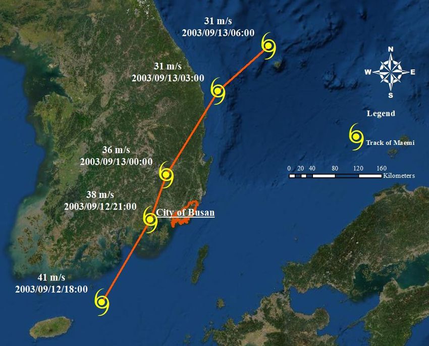
1.2.2 Tidal-gauge stations in South Korea This study focuses on the 15 tidal-gauge stations located
on the southern and western coasts (Fig. 2). The reason for
Effective measures for reducing the damage caused by future excluding the remaining two stations is that the majority of
typhoons, especially the design and re-design of waterfront typhoons do not arrive from the east or make landfall on
infrastructure, will require accurate prediction of storm-surge that coast. The hourly tidal data for this study have been
https://doi.org/10.5194/nhess-2121-2611-20212021 Nat. Hazards Earth Syst. Sci., 2121, 2611–2631, 20212021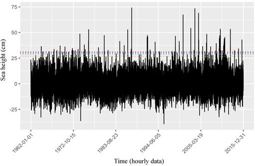
2614              S.-G. Yum et al.: Estimation of the non-exceedance probability of extreme storm surges in South Korea

Figure 2. Locations of the 15 tidal-gauge stations on the western and southern coasts of South Korea as of 2003. The locations of tidal-gauge
stations were created by the authors using the base map provided by ArcGIS.

provided by the Korea Hydrographic and Oceanographic                     Table 4. The three highest water levels recorded at each tidal-gauge
Agency (KHOA, 2019) and are used with that agency’s per-                 station on South Korea’s west coast.
mission.
                                                                              Location      Years     Top     Dates and times of peaks
                                                                                           of data   three    (GMT+9)
1.2.3   Highest recorded water levels
                                                                                                     peaks
                                                                                                     (cm)
The western tidal-gauge stations are located at Incheon,
Gyeongin, Changwon, Gunsan, and Mokpo. These five sta-                                                987     24 Jul 2013, 10:00
tions have operated for different lengths of time, ranging                    Incheon          18     981     8 Sep 2002, 06:00
from 2 to 61 years. Collection of the sea levels observed                                             980     27 Oct 2003, 18:00
hourly by each station throughout their respective periods                                            993     30 Sep 2015, 19:00
of operation revealed the top three sea-level heights at each.                Gyeonin           2     987     29 Sep 2015, 18:00
These heights, which are shown in Table 4, are clearly corre-                                         986     29 Oct 2015, 18:00
lated with the dates of arrival of typhoons.                                                          798     30 Sep 2015, 17:00
   The same approach was applied to the data from the                         Janghang         14     796     11 Oct 2014, 17:00
10 tidal-gauge stations on the south coast, as shown in Ta-                                           794     29 Sep 2015, 16:00
bles 5 and 6.
                                                                                                      805     19 Aug 1997, 04:00
                                                                              Gunsan           37     799     21 Aug 1997, 05:00
1.2.4   Tidal-gauge station at the city of Busan in South
                                                                                                      797     31 Aug 2000, 05:00
        Korea
                                                                                                      544     4 Jul 2004, 04:00
One of the focal tidal-gauge stations has observation records                 Mokpo            61     544     6 Jul 2004, 05:00
covering more than half a century. It is located on the south                                         538     16 Nov 2012, 16:00
coast at Busan, South Korea’s second-largest city. Thanks
to its location near the sea, Busan’s international trade has

Nat. Hazards Earth Syst. Sci., 2121, 2611–2631, 20212021                         https://doi.org/10.5194/nhess-2121-2611-20212021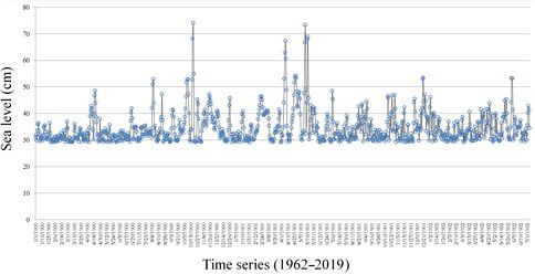
S.-G. Yum et al.: Estimation of the non-exceedance probability of extreme storm surges in South Korea                                         2615

Table 5. The three highest water levels recorded at 9 of the 10 tidal-
gauge stations on South Korea’s south coast.

    Location              Years of     Top    Dates/times of peaks
                             data     three   (GMT+9)
                                      peaks
                                      (cm)
                                      221     18 Sep 2012, 10:00
    Port of New Busan           5     219     17 Sep 2012, 09:00
                                      219     11 Aug 2014, 21:00
                                      252     17 Sep 2012, 10:00
    Gadeok                     40     246     17 Sep 2012, 09:00
                                      246     16 Jul 1987, 00:00
                                                                         Figure 3. Mean sea-level fluctuations in Busan, South Korea, 1962–
                                      265     17 Sep 2012, 10:00         2019 (KHOA, 2019).
    Masan                      37     264     17 Sep 2012, 11:00
                                      244     29 Aug 2004, 21:00
                                      133     19 Aug 2004, 08:00         Table 7. Kolmogorov–Smirnov normality test of sea-level fluctua-
    Ulsan                      55     120     12 Sep 2003, 21:00         tion data from the Busan tidal-gauge station.
                                      129     17 Sep 2012, 20:00
                                      426     12 Sep 2003, 21:00                                  Statistic    Degrees of    Significance    Pearson
                                                                                                              freedom (df)                  correlation
    Tongyeong                  41     357     12 Sep 2012, 10:00
                                      356     12 Sep 2003, 20:00          Sea-level fluctuation    0.084        473 352         0.200          0.96
                                      352     30 Aug 2015, 22:00
    Samcheonpo                  2     350     28 Oct 2015, 09:00
                                      350     27 Nov 2015, 10:00
                                                                         ble 6. As this table indicates, all of the top three water heights
                                      270     17 Sep 2012, 09:00
                                                                         recorded in the long history of this station occurred during
    Geoje                      11     259     17 Sep 2012, 10:00
                                      255     4 Jan 2006, 09:00          Typhoon Maemi’s passage through the area.
                                                                            KHOA makes hourly observations of water height at the
                                      479     17 Sep 2012, 10:00
                                                                         Busan tidal-gauge station, and the annual means presented in
    Gwangyang                   6     443     17 Sep 2012, 11:00
                                      441     1 Aug 2014, 22:00          this paper have been calculated from that hourly data. As can
                                                                         be seen in Fig. 3, plotting MSL for each year confirms that
                                      440     18 Aug 1966, 23:00
                                                                         short-term water-level variation merely masks the long-term
    Yeosu                      52     430     14 Sep 1966, 21:00
                                      129     17 Aug 1966, 22:00         trend of sea-level increase. Therefore, on the assumption that
                                                                         MSL variation was a function of time, a linear regression was
                                                                         performed, with the resulting coefficient of slope indicating
Table 6. The three highest water levels recorded at the tidal-gauge      the rate of increase (Yoon and Kim, 2012). The data utilized
station in Busan, South Korea.                                           to estimate MSL for the tidal-gauge station in Busan were
                                                                         provided by KHOA, which performed quality control on the
                    Years      Top      Dates/times of peaks             data before releasing it to us. Additionally, however, a nor-
                   of data    three               (GMT+9)                mality test was performed, and the results (as shown in Ta-
                              peaks
                                                                         ble 7) indicated that the hourly sea-level data followed a nor-
                              (cm)
                                                                         mal distribution at a significance > 0.05. The Kolmogorov–
                               211       12 Sep 2003, 21:00              Smirnov normality test was adopted as it is well suited to
         Busan       54        190       12 Sep 2003, 20:00              datasets containing more than 30 items.
                               188       12 Sep 2003, 12:00                 As can be seen in Fig. 3, the average rate of increase in
                                                                         MSL at Busan’s tidal-gauge station from 1962 to 2019 was
                                                                         2.4 mm yr−1 , yielding a difference of 16.31 cm between the
boomed, and as a consequence it now boasts the largest port              beginning and the end of that period. This finding is broadly
in South Korea. The Nakdong, the longest and widest river                in line with the Yoon and Kim (2012) finding that the rate
in South Korea, also passes through it. Due to these geo-                of MSL increase around the Korean Peninsula as a whole
graphical characteristics, Busan has been very vulnerable to             between 1960 and 2010 was about 2.9 mm yr−1 . In addi-
natural disasters, and the importance of accurately predicting           tion, linear-regression analysis of the sea-level fluctuation
the characteristics of future storms is increasingly recognized          data for 1965–2019 was utilized to discern the MSL trend.
by its government and other stakeholders. The top three sea-             The significance level of 0.000 (< 0.05) obtained via analy-
level heights at the tidal-gauge station there are shown in Ta-          sis of variance (ANOVA; Table 8) indicates that the regres-

https://doi.org/10.5194/nhess-2121-2611-20212021                         Nat. Hazards Earth Syst. Sci., 2121, 2611–2631, 20212021
2616              S.-G. Yum et al.: Estimation of the non-exceedance probability of extreme storm surges in South Korea

Table 8. Linear-regression coefficients and sea-level fluctuations at the Busan tidal-gauge station.

                                                Non-standardized coefficients     Standardized           t     Significance
                                                Coefficients         Standard         beta                     probability
                                                          B              error                                  (p value)
                     (Constant)                    −422.23             35.022        0.887        −12.06          0.00
                     Sea-level fluctuations          0.246              0.018                      13.97          0.00

Table 9. Summary of the analysis of variance results and sea-level fluctuations at the Busan tidal-gauge station.

                   Model                      Sum of           df           Mean        F         Significance      Adjusted
                                              squares                     squares                 level (Sig.)        R2
                   Regression       830 446 354.04           41     20 254 789.12    32 109.38         0.000          0.74
                   Residual         298 566 787.86      473 310            630.81
                   Total          1 129 013 141.90      473 351

sion model of sea-level fluctuations was significant. Its cor-            2      Literature review
relation coefficient (0.96) also indicated a strong positive re-
lationship between sea-level rise and recentness. The coef-               2.1     Prior studies of Typhoon Maemi
ficient of determination (R 2 ) was utilized to describe how
well the model explained the collected data. The closer R 2               Most previous studies devoted to avoiding or reducing nat-
is to 1, the better the model can predict the linear trend: here          ural disaster damage in South Korea have focused on storm
it was 0.74, as shown in Table 9. This means that the linear-             characteristics, such as storm track, rainfall, radius, and wind
regression model explained 74 % of the sea-level variation.               field data. Their typical approach has been to create synthetic
While this result suggests that the linear-regression analysis            storms that can be utilized to predict real storm paths and es-
for sea-level fluctuation at the tidal-gauge station in Busan is          timate the extent of the damage they would cause.
reliable, such results may not be generalizable because varia-               Kang (2005) investigated the inundation and overflow
tion in the data could have been due to several factors, includ-          caused by Typhoon Maemi at one location near the coast,
ing geological variation and modification of gauge points.                using a site survey and interviews with residents, and found
                                                                          that the storm surge increased water levels by 80 %. Using
1.2.5   Relationship between sea level and typhoons                       a numerical model, Hur et al. (2006) estimated storm surges
                                                                          at several points in the Busan area caused by the most se-
When a storm occurs, surge height tends to increase, and                  rious typhoons, including Sarah, Thelma, and Maemi. Hav-
these larger surges can cause natural disasters such as floods.           ing established that Maemi was accompanied by the highest
In this study, before calculating the height of a surge, we took          storm surge, they then simulated storm surges as a means
account of the dates and times when the three greatest sea-               of investigating the tidal characteristics of Busan’s coast and
level heights were observed, as well the dates and times when             created virtual typhoons to compare against the actual tracks
typhoons occurred. These data are presented side by side in               of Sarah, Thelma, and Maemi. When these virtual typhoons
Table 10.                                                                 followed the track of Typhoon Maemi, their simulated storm
   As Table 10 indicates, the top three recorded sea levels at            surges were higher than the ones produced by those that fol-
each south coast tidal-gauge station corresponded with the                lowed the other two tracks.
occurrence of typhoons in 20 out of 30 cases. Moreover, the                  Lee et al. (2008), using atmospheric-pressure and wind
dates and times of the three highest sea levels observed dur-             profiles of Typhoon Maemi, introduced a multi-nesting grid
ing all 57 years’ worth of data from Busan all coincided with             model to simulate storm surges. To check its performance,
Typhoon Maemi passing out of the area.                                    they used numerical methods for tidal calibration and to as-
   As well as USD 3.5 billion in property damage, Typhoon                 sess the influence of open-boundary conditions and typhoon
Maemi caused 135 casualties in Busan and nearby cities (Na-               paths. This yielded two key findings. First, the location of a
tional Typhoon Center, 2011). However, other typhoons –                   typhoon’s centre was the most critical factor when calculat-
notably including Thelma, Samba, and Megi – also caused                   ing storm surges. Second, the track of the typhoon was a sec-
considerable damage, as shown in Table 1.                                 ondary, but still important, factor in storm-surge prediction.
                                                                          However, the research of Lee et al. (2008) was limited by the
                                                                          fact that only recorded storm tracks were used, meaning that

Nat. Hazards Earth Syst. Sci., 2121, 2611–2631, 20212021                            https://doi.org/10.5194/nhess-2121-2611-20212021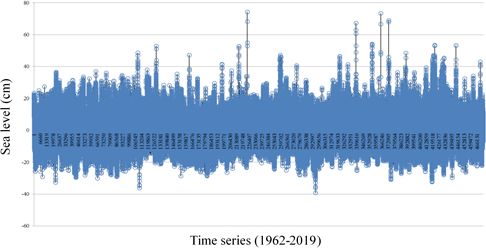
S.-G. Yum et al.: Estimation of the non-exceedance probability of extreme storm surges in South Korea                                  2617

Table 10. Relationship between sea level and typhoons on the south           the exceedance probabilities of storm surges. For instance,
coast of South Korea.                                                        Kim and Suh (2018) did not perform surge modelling or fre-
                                                                             quency analysis in the time domain, and although the numer-
 Location                      Years   Peak   Date                 Typhoon
                                                                             ical models of Chun et al. (2008) provided valuable predic-
                                       (cm)   (GMT+9)
                                                                             tions of inundation area and depth, they did not take account
                                       211    12 Sep 2003, 21:00   Maemi     of tidal fluctuation, which if combined with increased water
 Busan                           54    190    12 Sep 2003, 20:00   Maemi
                                       188    12 Sep 2003, 12:00   Maemi
                                                                             levels would have yielded different results.
                                                                                Using insurance data from when Typhoon Maemi made
                                       221    18 Sep 2012, 10:00   Sanba
                                                                             landfall on the Korean Peninsula, Yum et al. (2021) presented
 Port of New Busan                5    219    17 Sep 2012, 09:00   Sanba
                                       215    18 Sep 2012, 22:00   Sanba     vulnerability functions linked to typhoon-induced high wind
                                                                             speeds. Specifically, the authors used insurance data to calcu-
                                       252    17 Sep 2012, 10:00   Sanba
 Gadeok                          40    246    17 Sep 2012, 09:00   Sanba
                                                                             late separate damage ratios for residential, commercial, and
                                       246    16 Jul 1987, 00:00   Thelma    industrial buildings and four damage states adopted from an
                                                                             insurance company and a government agency to construct
                                       265    17 Sep 2012, 10:00   Sanba
 Masan                           37    264    17 Sep 2012, 11:00   NA        vulnerability curves. The mean-squared error and maximum-
                                       244    29 Aug 2004, 21:00   NA        likelihood estimation (MLE) were used to ascertain which
                                       133    19 Aug 2004, 08:00   Megi      curves most reliably explained the exceedance probability of
 Ulsan                           55    120    12 Sep 2003, 21:00   Maemi     the damage linked to particular wind speeds. Making novel
                                       129    17 Sep 2012, 20:00   Sanba     use of a binomial method based on MLE, which is usually
                                       426    12 Sep 2003, 21:00   Maemi     used to determine the extent of earthquake damage, the same
 Tongyeong                       41    357    12 Sep 2012, 10:00   Sanba     study found that such an approach explained the extent of the
                                       356    12 Sep 2003, 20:00   Maemi     damage caused by high winds on the Korean Peninsula more
                                       352    30 Aug 2015, 22:00   NA        reliably than other existing methods, such as the theoretical
 Samcheonpo                       2    350    28 Oct 2015, 09:00   NA        probability method.
                                       350    27 Nov 2015, 10:00   NA
                                       270    17 Sep 2012, 09:00   Sanba     2.2   Return period estimates for Hurricane Sandy
 Geoje                           11    259    17 Sep 2012, 10:00   Sanba
                                       255    4 Jan 2006, 09:00    NA
                                                                             While no prior research has estimated return periods for ty-
                                       479    17 Sep 2012, 10:00   Sanba     phoons, some studies have done so for hurricanes. For ex-
 Gwangyang                        6    443    17 Sep 2012, 11:00   Sanba     ample, Talke et al. (2014) used tidal-gauge data to study the
                                       441    1 Aug 2014, 22:00    NA
                                                                             storm-surge hazard in New York Harbor over a 37-year pe-
                                       440    18 Aug 1966, 23:00   NA        riod and found that its pattern underwent long-term changes
 Yeosu                           52    430    14 Sep 1966, 21:00   NA
                                                                             due to sea-level rise caused in part by climate change. How-
                                       129    17 Aug 1966, 22:00   NA
                                                                             ever, Talke et al. (2014) did not estimate a specific return
NA stands for not available.
                                                                             period for Hurricane Sandy, which struck the United States
                                                                             in 2012.
                                                                                Lin et al. (2010), on the other hand, did estimate the return
their simulations could not calculate storm surges from any                  periods of storm surges related to tropical cyclones in the
other possible tracks. Similarly, Chun et al. (2008) simulated               New York City area, with that for Sandy in Lower Manhat-
the storm surge of Typhoon Maemi using a numerical model,                    tan being 500 years within a 95 % CI (confidence interval),
combined with moving boundary conditions to explain wave                     i.e. approximately 400–700 years. Lin et al. (2012) later con-
run-up, but using data from the coastal area of Masan: a city                ducted a similar analysis using computational fluid dynamics
near Busan that was also damaged by the storm. The inun-                     Monte Carlo simulations that took account of the random-
dation area and depth predicted by the model of Chun et                      ness of the tidal-phase angle. This approach yielded a return
al. (2008) were reasonably well correlated with the actual                   period of 1000 years with a 90 % CI (750–1050 years). The
area and depth arrived at via a site survey. Lastly, Kim and                 former study can be considered the less accurate of the two
Suh (2018) created 25 000 random storms by modifying an                      because it did not consider different surge height possibilities
automatic storm-generation tool, the Tropical Cyclone Risk                   at different time windows within the tidal cycle.
Model, and then simulated surge elevations for each of them.                    Hall and Sobel (2013) developed an alternative method
The tracks of these simulated storms had similar patterns to                 to estimate Sandy return periods, based on the insight that
those of actual typhoons in South Korea.                                     this storm’s track could have been the primary reason for the
   However, while past research on Typhoon Maemi has used                    damage it caused in Lower Manhattan and other parts of the
such input data as tidal-gauge data, atmospheric pressure,                   city. Specifically, they argued that Sandy’s perpendicular im-
wind fields, typhoon radius, storm speed, latitude, and lon-                 pact angle with respect to the shore as it passed to the south
gitude, tidal-gauge data has not been used for estimating                    of Manhattan’s port was of critical importance, based on an

https://doi.org/10.5194/nhess-2121-2611-20212021                             Nat. Hazards Earth Syst. Sci., 2121, 2611–2631, 20212021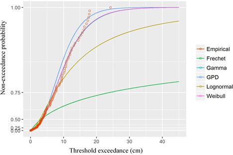
2618              S.-G. Yum et al.: Estimation of the non-exceedance probability of extreme storm surges in South Korea

analysis of the tracks of other hurricanes of similar intensity.     relation between extreme events and flood drivers. They also
They estimated the return period for Sandy’s water level to          adopted ordinary least-squares regression analysis to con-
be 714 years within a 95 % CI (435–1429 years).                      struct a 10 000-year time series and computed water levels’
    Zervas (2013) estimated the return periods for extreme           exceedance probabilities for comparison. However, the pos-
events using monthly mean water-level data from the                  sibility of river discharges, sea-wave trends, and tidal fluctu-
US National Oceanographic and Atmospheric Administra-                ations were not considered in their study.
tion, recorded at the tidal-gauge station in Battery Park,              The wrecking of wind farms by extreme windstorms is
New York. Using GEV distribution and MLE, Zervas cal-                of considerable concern in the North Sea region, which is
culated that the return period for Sandy’s peak water level          home to 38 such farms belonging to five different coun-
was 3500 years, but sensitivity analysis suggested that the          tries. According to the Monte Carlo simulation-based risk-
estimated results were probably inaccurate, given the GEV            management study of Buchana and McSharry (2019), the to-
fit’s sensitivity to the range of years used. Once Sandy was         tal asset value of these wind farms is EUR 35 billion. It used
excluded, the return period was 60 000 years. This difference        a log-logistic damage function and Weibull probability distri-
in results suggests that GEV distribution of the yearly maxi-        bution to assess the risks posed to wind farms in that region
mum water level is not a realistic method for estimating ex-         by extreme strong wind and exceedance probability to pre-
treme events in the New York Harbor area.                            dict the extent of financial loss from such damage in terms
    Building on her own past research, Lopeman (2015) – the          of solvency capital requirement (SCR). The same study also
first researcher to estimate Sandy’s return period using tidal-      simulated the results of various climate change scenarios,
gauge data – proposed that a clustered separated peaks-over-         and the results confirmed that higher wind speed and higher
threshold (POT) method (CSPS) should be used and that tide           storm frequency were correlated with rises in SCR: a finding
fluctuation, surge, and sea-level rise should all be dealt with      that could be expected to help emergency planners, investors,
separately because out of these three phenomena only surge           and insurers reduce their asset losses.
is truly random. This approach led Lopeman to calculate the             According to a study by Catalano et al. (2019) of high-
return period as 103 years with a 95 % CI (38–452 years).            impact extratropical cyclones (ETCs) on the northeastern
    Zhu et al. (2017) explored recovery plans pertaining to          coast of the Unites States, limited data caused by these
two New York City disasters, Hurricane Irene and Hurricane           storms’ rarity made it difficult to predict the damage they
Sandy, using data-driven city-wide spatial modelling. They           would cause or analyse their frequency. To overcome this,
used resilience quantification and logistic modelling to de-         they utilized 1505 years’ worth of simulations derived from
lineate neighbourhood tabulation areas, which were smaller           a long coupled model, GFDL FLOR, to estimate these ex-
units than other researchers had previously used and enabled         treme events’ exceedance probabilities and compared the re-
the collection of more highly detailed data. They also intro-        sults against those of short-term time series estimation. This
duced the concept of “loss of resilience” to reveal patterns         not only revealed that the former was more useful for sta-
of recovery from these two hurricanes, again based on their          tistical analysis of ETCs’ key characteristics – which they
smaller spatial units. Moran’s I was utilized to confirm that        defined as maximum wind speed, lowest pressure, and surge
loss of resilience was strongly correlated not only with spa-        height – but also that the use of a short time series risked
tial characteristics but also with socioeconomic characteris-        biassing estimates of ETCs’ return levels upwards (i.e. un-
tics and factors like the location of transport systems. How-        derestimating their actual frequency). While these results re-
ever, given the particularity of such factors, the results of Zhu    garding return levels and time series were valuable, Catalano
et al. (2017) might not be generalizable beyond New York             et al. (2019) did not distinguish between the cold season and
City, and they made no attempt to predict future extreme             the warm season of each year, which could also have led to
events’ severity or frequency.                                       biased results.
    The sharp differences in the results of the past studies cited      A joint-probability methodology was used to analyse ex-
above are due to wide variations in both the data they used          treme water heights and surges on China’s coast by Chen
and their assumptions. The present study therefore applies all       et al. (2019). They obtained the sea-level data from nine
of the methods used in previous studies of Hurricane Sandy’s         gauge stations, and utilized 35 years’ worth of simulation
return period to estimate that of Typhoon Maemi and in the           data with a Gumbell distribution and a Gumbell–Hougaard
process establishes a new model.                                     copula. The three major sampling methods proposed in the
                                                                     study were structural-response, wave-dominated, and surge-
2.3     Extreme value statistics                                     dominated sampling. The first was utilized to assess struc-
                                                                     tures’ performance in response to waves and surges. Joint-
2.3.1    Prior studies of extreme natural hazards                    probability analysis revealed that such performances were
                                                                     correlated with extreme weather events in the target region
Bermúdez et al. (2019) studied flood drivers in coastal and          and that such correlations became closer when wave motion
riverine areas as part of their approach to quantifying flood        was stronger. In addition, based on their finding that joint
hazards, using 2D shallow-water models to compute the cor-           exceedance probability tended to overestimate return periods

Nat. Hazards Earth Syst. Sci., 2121, 2611–2631, 20212021                    https://doi.org/10.5194/nhess-2121-2611-20212021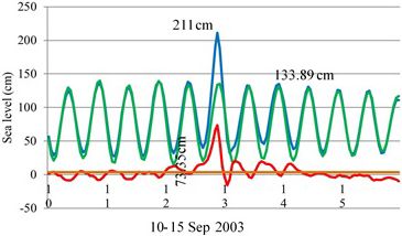
S.-G. Yum et al.: Estimation of the non-exceedance probability of extreme storm surges in South Korea                      2619

for certain water levels, Chen et al. (2019) recommended that    lated typhoons as a means of predicting the cost of the dam-
offshore defence facility designers use joint-probability den-   age they would cause in Tokyo Bay, which is very vulnera-
sity to estimate return levels of extreme wave heights. How-     ble to such events due to its geographic and socio-economic
ever, while their study provided a useful methodology, partic-   characteristics. Using stochastic approaches, they modelled
ularly with regard to sampling methods and probability mod-      future typhoons over a 10 000-year period and calculated
elling of return periods and structural performance, they only   flooding using a numerical surge model based on the prob-
looked at China’s coast, and therefore their findings are un-    ability of historical typhoons. These flooding calculations, in
likely to be generalizable to the Korean Peninsula.              turn, were utilized to create a storm-surge inundation map,
   Davies et al. (2017) proposed a framework for probabil-       representing exceedance probabilities derived from stochas-
ity modelling of coastal storm surges, especially during non-    tic hazard calculations pertaining to 1000 typhoons. Next, the
stationary extreme storms and tested it using the El Niño–       completed map was overlaid on government-provided values
Southern Oscillation (ENSO) on the east coast of Aus-            of Tokyo Bay’s buildings and other infrastructural elements
tralia. Importantly, they applied their framework to ENSO        to assess the spatial extent and distribution of the likely dam-
and seasonality separately. This is because while ENSO af-       age. The results showed that Chiba and Kanagawa would be
fects storm-wave direction, mean sea level, and storm fre-       the most damaged areas and would suffer financial losses of
quency, seasonality is mostly related to storm-surge height,     JPY 158.4 billion and 91.5 billion, respectively, with an ex-
storm-surge duration, and total water height. This separation    ceedance probability of 0.005 (as commonly used to estimate
has the advantage of allowing all storm variables of non-        damage in the insurance industry). However, the real estate
stationary events to be modelled, regardless of their marginal   values they used were 2 decades out of date at the time their
distribution. Specifically, Davies et al. (2017) applied non-    study was conducted, meaning that further validation of their
parametric distribution to storm-wave direction and steep-       approach will be needed.
ness and parametric distribution to duration and surge using        Another effort to estimate return periods was made by
mixture-generalized extreme value probability modelling,         McInnes et al. (2016), who created a stochastic dataset on all
which they argued was more useful than standard models           cyclones that occurred near Samoa from 1969 to 2009. That
like generalized Pareto distribution (GPD). They said this       dataset was utilized to model storm tides using an analytic
was because the statistical threshold in an extreme mixture      cyclone model and a hydrodynamic model, which also took
model can be integrated into the analysis, whereas a GPD         into account prevailing climate phenomena such as La Niña
model should be given an unbiased threshold: if it is low,       and El Niño when estimating return periods. The authors
too many normal data may be included. Accordingly, they          found that tropical cyclones’ tracks could be affected by
utilized bootstrapping for the confidence interval to show       La Niña and El Niño and, more specifically, that the fre-
the uncertainty of the non-stationary aspects of the extreme     quency of cyclones and storm tides during El Niño was con-
events. They also added a Bayesian method to provide wider       sistent across all seasons, whereas La Niña conditions make
confidence intervals with less bias. Their findings are mainly   their frequency considerably lower in the La Niña season.
beneficial to overcoming the challenges of GPD threshold         Additionally, McInnes et al. (2016) proposed that sea-level
selection; however, robust testing of their approach will re-    rise had a more significant influence on storm tides than fu-
quire that it be applied to a wider range of abnormal climate    ture tropical cyclones did, based on their finding that future
phenomena.                                                       cyclones’ frequency would be reduced as the intensity of fu-
   Similar research was conducted by Fawcett and Wal-            ture cyclones increased. Lastly, they found that the likelihood
shaw (2016), who developed a methodology for estimat-            of a storm tide exceeding a 1 % annual exceedance proba-
ing the return levels of extreme events such as sea surges       bility (i.e. a once a century tide) was 6 % along the entire
and high winds of particular speeds, with the wider aim of       coastline of Samoa. However, other effects such as sea-level
informing practical applications such as design codes for        fluctuations and meteorological factors were not included in
coastal structures. They reported that two of the most pop-      their calculations.
ular existing methods for doing so, block maxima (BM) and           Silva-González et al. (2017) studied threshold estimation
POT, both have shortcomings and concluded that a Bayesian        for analysis of extreme wave heights in the Gulf of Mex-
approach would be more accurate. Specifically, they argued       ico and argued that appropriate thresholds for this purpose
that BM and POT methods tend to waste valuable data and          should consider exceedances. They applied the Hill estimator
that considering all exceedance via accurate estimation of the   method, an automated threshold-selection method, and the
extremal index (reflecting uncertainty’s natural behaviour)      square-error method for threshold estimation in hydrolog-
could compensate for this disadvantage. They further pro-        ical, coastal engineering, and financial scenarios with very
posed that the seasonal variations should be taken into con-     limited data and found that the square-error method had the
sideration with the all exceedance data, where possible.         most advantages because it did not consider any prior pa-
   In response to Japanese government interest in unexpected     rameters that could affect thresholds. The authors went on to
flooding caused by extreme storm surges during typhoons          propose improvements to that method, i.e. the addition of dif-
and other high-wind events, Hisamatsu et al. (2020) simu-        ferences between quantiles of the observed samples and me-

https://doi.org/10.5194/nhess-2121-2611-20212021                 Nat. Hazards Earth Syst. Sci., 2121, 2611–2631, 20212021
2620              S.-G. Yum et al.: Estimation of the non-exceedance probability of extreme storm surges in South Korea

dian quantiles from GPD-aided simulation. When GPD was                identified as extreme and converge to a GPD. The following
utilized to estimate observed samples, it effectively prevented       two subsections discuss the BM and POT methods as illus-
convergence problems with the maximum-likelihood method               trations of these two groups, respectively (Coles, 2001).
when only small amounts of data were available. The key
advantage of the approach of Silva-González et al. (2017) is          Block maxima method
that the choice of a threshold can be made without reliance
on any subjective criteria. Additionally, no particular choice        The BM approach relies on the distribution of the maximum
of marginal probability distribution is required to estimate          extreme values in the following equation,
a threshold. However, to be of practical value, their method          Mn = max {X1 , . . ., Xn } ,                                (1)
will need to incorporate more meteorological factors.
   Lastly, the Wahl et al. (2015) study of the exceedance             where the Xn series, comprising independent and identically
probabilities of a large number of synthetic and a small              random variables, occurs in order of maximum extreme val-
number of actual storm-surge scenarios utilized four steps:           ues, n is the number of observations in a year, and Mn is the
parameterizing the observed data, fitting different distribu-         annual maximum.
tion models to the time series, Monte Carlo simulation, and              Data is divided into blocks of specific time periods, with
recreating synthetic storm-surge scenarios. Specifically, pro-        the highest values within each block collectively serving as
jected 40 and 80 cm sea-level rises were used as the basis            a sample of extreme values. One limitation of this method
for investigating the effects of climate change on flooding           is the possibility of losing important extreme value data be-
in northern Germany. Realistic joint exceedance probabili-            cause only the single largest value in each block is accounted
ties were used for all parameters with copula models, and             for, and thus the second-largest datum in one block could be
the exceedance probabilities of storm surges were obtained            larger than the highest datum in another.
from the bivariate exceedance probability method with two
parameters, i.e. the highest total water level with the tidal         Peaks-over-threshold method
fluctuations and intensity. The findings of Wahl et al. (2015)
indicated that extremely high water levels would cause sub-           The POT method can address the above-mentioned limita-
stantial damage over a short time period, whereas relatively          tions of BM, insofar as it can gather all the data points that
small storm surges could inflict similar levels of damage but         exceed a certain prescribed threshold and use limited data
over a much longer period. However, like various other stud-          more efficiently because it relies on relatively large or high
ies cited above, Wahl et al. (2015) did not take seasonal vari-       values instead of the largest or highest ones. All values above
ation into account.                                                   the threshold – known as exceedances – can be explained by
                                                                      the differentiated tail data distribution. The basic function of
2.3.2   Generalized extreme value distribution                        this threshold is to assort the larger or higher values from
                                                                      all data, and the set of exceedances constitutes the sample
Extreme events are hard to predict because data points are            of extreme values. This means that although POT can cap-
so few, and predicting their probability is particularly diffi-       ture potentially important extreme values even when they oc-
cult due to their asymptotic nature. Extreme value probabil-          cur close to each other, selecting a threshold that will yield
ity theory deals with how to find outlier information, such           the best description of the extreme data can be challenging
as maximum or minimum data values, during extreme situa-              (Bommier, 2014); i.e. if it is set too high, key extreme val-
tions. Examining the tail events in a probability distribution        ues might be lost, but if it is set too low, values that are not
is very challenging. However, it is considered very important         really extreme may be included unnecessarily. Determining
by civil engineers and insurers due to their need to cope with        appropriate threshold values thus tends to require significant
low-probability, high-consequence events. For example, the            trial and error, and various studies have proposed methods
designs and insurance policies of bridges, breakwaters, dams,         for optimizing such values (Lopeman et al., 2015; Pickands,
and industrial plants located near shorelines or other flood-         1975; Scarrott and Macdonald, 2012). Pickands (1975), for
prone areas should account for the probability, however low,          instance, suggested that independent time series that exceed
of major flooding. Various probability models for the study           high enough thresholds would follow GPD asymptotically,
of extreme events could potentially be used in the present re-        thus avoiding the inherent drawbacks of BM. The distribu-
search, given that its main topic is the extreme high water           tion function F of exceedance can be computed as
levels caused by typhoons. Extreme value theories can be di-
                                                                      Fθ (x) = P {X − θ ≤ x|X > θ } , x ≥ 0,                      (2)
vided into two groups, according to how they are defined. In
the first, the entire interval of interest is divided into a number   where θ is the threshold and X is a random variable.
of subintervals. The maximum value from each subinterval is             Fu , meanwhile, can be defined by conditional probabilities
identified as the extreme value, and following this the entirety                F (θ+x)−F (θ)
of these extreme values converge into a GEV distribution. In                         1−F (θ)     if x ≥ 0
                                                                      Fθ (x) =                             .                    (3)
the second group, values that exceed a certain threshold are                      0              else

Nat. Hazards Earth Syst. Sci., 2121, 2611–2631, 20212021                      https://doi.org/10.5194/nhess-2121-2611-20212021
S.-G. Yum et al.: Estimation of the non-exceedance probability of extreme storm surges in South Korea 2621
According to Bommier (2014), the distribution of ex-
ceedances (Y1 , . . . , Ynθ ) can be generalized by GPD with
the following assumption: when Y = X − θ for X > θ , and
X1 , . . . , Xn , Yj = Xi − θ can be described with i, which is
the j th exceedance, i = 1, . . . , nθ .
The GPD can be expressed as
1 − 1 + ξ (x−θ) 1/ξ ξ 6 = 0
σ
Gx (x; ξ, σ, θ ) = (4)
1 − exp − (x−θ) ξ = 0,
σ
with x being independent and identically random variables,
σ the scale, ξ the shape, and θ the threshold. All values above
θ are considered tail data (extreme values). The probabil-
ity of exceedance over a threshold when calculating a return
level that is exceeded once every N years (N -year return pe-
riods xN ) is calculated as follows:
Figure 4. General approach and workflow.
x − θ −1/ξ
P {X > x|X > θ } = 1 + ξ . (5)
σ
If the exceedances above the threshold are rare events λ (as are therefore expected to provide a viable method of pre-
measured by number of observations per year), we can ex- dicting economic losses associated with typhoons and corre-
pect P (X > θ ) to follow Poisson distribution. The mean of sponding models for managing emergency situations arising
exceedance per unit of time (γ̂ ) describes that distribution. from natural disasters that can be used by South Korea’s gov-
ernment agencies, insurance companies, and construction in-
γ dustry. Although this study focuses on a specific city-region,
P (X > θ ) = (6)
λ its proposed probabilistic methodologies should also be ap-
In other words, γ can be estimated by dividing the number plicable to other coastal regions in South Korea and around
of exceedances by the number of years in the observation the world.
period. To explore the non-exceedance probability of storm
Combining the POT and Poisson processes with GPD al- surges, this study utilized tidal-gauge data from the city of
lows us to describe the conditional probability of the extreme Busan, collected when Typhoon Maemi struck it in 2003.
values that exceed the designated threshold, as per Eq. (7) As shown in Fig. 4, we proceeded according to several
(Lopeman et al., 2015): steps. First, the observed tidal-gauge data were utilized to
calculate the predicted water level through harmonic anal-
P (A ∩ B) ysis and then the storm surge height, which is the differ-
P (A|B) = . (7)
P (B) ence between observed and predicted water height. Second,
threshold and clustering techniques were applied to select
In addition, when Bayes’ theorem is applied to the role of data meaningful to the non-exceedance probabilities of ex-
GPD in conditional probability, we can rewrite Eq. (7) as fol- treme storm surges. Third, the extreme values were sepa-
lows: rated into cold-season and warm-season categories to boost
P (θ < X < x) the reliability of our probability distribution model. Fourth,
GX (x) = . (8) the maximum-likelihood method was used to estimate non-
P (X > θ )
exceedance probability. Finally, various probability models
were built, and the one that best fit the empirical data was
3 Research methods identified.
The objective of this study is to estimate the probability of
3.1 Data processing
the risk, for each year, of typhoon-induced high water lev-
els in Busan. To that end, it adapts Lopeman et al.’s (2015)
CSPS, which provides statistical analysis of extreme values 3.1.1 Storm-surge data collection method
in long time series of natural phenomena. As such, CSPS can
provide useful guidance to those tasked with preparing for To determine the height of surges from publicly available
natural disasters on the Korean Peninsula and perhaps on its KHOA data, it was first necessary to predict sea levels. Equa-
southern coast in particular. The findings from this research tion (9) explains the interrelationship of observed water level,
https://doi.org/10.5194/nhess-2121-2611-20212021 Nat. Hazards Earth Syst. Sci., 2121, 2611–2631, 202120212622 S.-G. Yum et al.: Estimation of the non-exceedance probability of extreme storm surges in South Korea
predicted water level, tidal-fluctuation height, and residual
(surge) at time ti ,
Yi = Xi + Si , (9)
where i = 1, 2, . . . , n, n is the time series of the input dataset,
Xi is the predicted water height at ti , Yi is the observed water
height at ti , and Si is the surge height.
3.1.2 Separation of tidal-gauge data via harmonic
analysis
A standard harmonic analysis was performed to calculate
predicted sea-level height based on hourly tidal-gauge data.
Figure 5. Observed (green), predicted (blue), and residual (red) wa-
First, this technique was used to estimate the tidal compo- ter levels at Busan during Typhoon Maemi.
nents of all seawater-level data, allowing residuals to be iso-
lated so that surge data could be calculated once sea-level
rise had been estimated. Second, the estimated constituents where βm,1 = Hm cos(gm ) and βm,2 = Hm sin(gm ). What is
were used to predict tidal fluctuations in the years simulated gained from this new representation is a linear function with
via Monte Carlo. Then, the TideHarmonics package in R respect to the parameters βm,1 and βm,2 that need to be es-
(Stephenson, 2017) was used to estimate tidal components, timated, and hence linear regression can be used. Given the
as detailed below. large time span covered by the data, M = 60 harmonic tidal
Given a time series Y (t) of total water levels, with t de- constituents were estimated, and a constant mean sea level Z
noting time in hours, the tidal component with M harmonic was assumed across all years of available data.
constituents is computed as
M
3.1.3 Observed, predicted, and residual water levels
X π
Ŷ (t) = Z + Am cos (ωm t − ψm ) , (10)
180 Because observed sea level usually differs from predicted sea
m=1
level, Fig. 5 depicts the former (as calculated through har-
where ωm is the angular frequency of the mth component monic analysis) in blue. Predicted sea levels are shown in
in degrees per hour. The 2M + 1 parameters to be estimated green, and surge height is shown in red. As the figure indi-
are the amplitudes Am , the phase lag ψm in degrees, and the cates, the highest overall water level coincided with the high-
MSL Z. est surge during Typhoon Maemi, i.e. at 21:00 GMT+9 on
To account for long astronomical cycles (LACs), nodal- 12 September 2003. Given a total water height of 211 cm, the
correction functions for both the amplitude and phase are surge height was calculated as 73.35 cm. The unexpectedly
used. With these corrections, the tidal component takes the large height of the surge induced by Typhoon Maemi caused
following form: USD 3.5 billion in property damage and many causalities in
M
Busan, as mentioned in Table 1.
X π
ŶLAC (t) = Z + Hm fm (t) cos (ωm t − gm
180 3.2 Data analysis
m=1
+um (t) + Vm )) , (11) 3.2.1 Threshold and target-rate selection
where fm (t) and um (t) represent the nodal corrections for At a given annual target rate – i.e. number of storms per
the amplitude and phase, respectively. In this new formula- year – the algorithm proposed by Lopeman et al. (2015)
tion, the amplitude and phase parameters to be estimated are (Fig. 6) computes the threshold such that this rate approxi-
denoted by Hm and gm (in degrees). Finally, Vm is the refer- mates the resulting yearly number of “exceedance clusters”,
ence signal, by which the phase lag gm is calculated and set i.e. consecutive surge observations that lie above the thresh-
to refer to the origin t = 0. old. Hence, rather than choosing an “ideal” threshold accord-
The summation term in ŶLAC (t) can alternatively be writ- ing to some other criterion, the algorithm simply finds the
ten as follows: threshold that forces a chosen target rate to occur. Accord-
M
X π ingly, a study of this kind could set its target rate as the av-
βm,1 fm (t) · cos (ωm t + um (t) + Vm ) erage rate observed over a given period or as a value that
180
m=1 the researchers find reasonable in light of their knowledge of
M
X π historical data for their focal area.
+ βm,2 fm (t) · sin (ωm t + um (t) + Vm ) , (12)
m=1
180
Nat. Hazards Earth Syst. Sci., 2121, 2611–2631, 20212021 https://doi.org/10.5194/nhess-2121-2611-20212021S.-G. Yum et al.: Estimation of the non-exceedance probability of extreme storm surges in South Korea 2623
Figure 6. Threshold-selection flowchart.
Next, the algorithm iteratively updates the threshold to 3. If the annual storm rate arrived at in step (1) is not close
allow a computationally intensive (but not exhaustive) ex- to the chosen target, the following steps are taken.
ploration of possible threshold values between its minimum
value (i.e. here the minimum observed surge height) and a. If it is smaller than the target rate, then the threshold
its maximum value (i.e. maximum observed surge height). from the previous iteration is the final result, and the
Specifically, it first sets the threshold to 0 cm and then itera- algorithm is stopped.
tively overwrites it according to the following steps. b. If it is larger than the target rate, then a vector col-
lecting the maximum height of the clusters is built
1. The exceedance clusters produced at a given iteration and sorted in descending order. The threshold is
and given threshold are identified, and the resulting an- then updated by setting it as equal to the Cth el-
nual storm rate computed. ement of this vector, where C is the integer clos-
2. If the annual storm rate arrived at in step (1) is equal est to 54 (i.e. the number of years covered by the
to (or about equal to) the chosen target, the threshold dataset) multiplied by the target rate. This updated
from the previous iteration is the final result, and the threshold is used in the next iteration of the algo-
algorithm is stopped. rithm, and steps (1) through (3) are repeated.
https://doi.org/10.5194/nhess-2121-2611-20212021 Nat. Hazards Earth Syst. Sci., 2121, 2611–2631, 202120212624 S.-G. Yum et al.: Estimation of the non-exceedance probability of extreme storm surges in South Korea
Figure 9. Iterative process of threshold selection (3 of 3).
Figure 7. Iterative process of threshold selection (1 of 3).
Figure 10. Various thresholds considered.
Figure 8. Iterative process of threshold selection (2 of 3).
3.2.2 Clustering of the storm-surge data:
interrelationship of target rate, threshold, and
As shown in Figs. 7–9, the threshold algorithm (Fig. 6) clusters
achieved convergence relatively quickly for all three target
rates selected, with the number of iterations required for con- Figures 7–9 show that, as expected, when the target rate
vergence ranging from three (with a target rate of 3.0) to five increases, the threshold decreases, and as the threshold de-
(with a target rate of 10). creases, the number of clusters (i.e. storm events) increases.
Figure 10 displays six possible thresholds. The first, Conversely, the lower the target rate, the lower the num-
31.2 cm, was based on a target rate of 3.5 and 189 clusters ber of clusters and the higher the threshold. Thus, if the
and is shown in red. The dark blue line represents the second desired number of storms is three per year, the algorithm
threshold of 30.54 cm, (target rate = 4.0; clusters = 217), the will converge in three iterations and set the threshold level
purple line shows a threshold of 29.56 cm (target rate = 4.5; to 32.01 cm; this results in a total of 164 storm events over
clusters = 246), the green line shows a threshold of 29.15 cm the time span covered by our data. Conversely, if the de-
(target rate = 5.0; clusters = 274), the sky blue line shows sired target rate is 10 storms per year, the threshold is signifi-
a threshold of 28.33 cm (target rate = 6.0; clusters = 324), cantly lower (25.43 cm), and the total number of storm events
and the orange line shows a threshold of 26.53 cm (target more than trebles to 539 clusters (Fig. 10). As can be seen
rate = 8.0; clusters = 431). in Fig. 11, we chose only one maximum value to represent
each cluster. Figures 12–14 show the stages of the clustering
of surges when the target rate is set to 5.0, the threshold is
29.15 cm, and the number of clusters is 274 (though it should
be noted that Fig. 12 indicates only the number of surges, due
to the difficulty of visually representing all surge dates and
Nat. Hazards Earth Syst. Sci., 2121, 2611–2631, 20212021 https://doi.org/10.5194/nhess-2121-2611-20212021You can also read