Communication algorithms and principles for a prototype of a wireless mesh network
←
→
Page content transcription
If your browser does not render page correctly, please read the page content below
Zachodniopomorski Uniwersytet Technologiczny
                w Szczecinie

          WYDZIAŁ INFORMATYKI

               Sergiusz Urbaniak
                Kierunek informatyka

Communication algorithms and principles for
  a prototype of a wireless mesh network

                      Praca dyplomowa magisterska
                      napisana pod kierunkiem
                      dr inż. Remigiusza Olejnika
                      w Katedrze Architektury Komputerów
                      i Telekomunikacji

                  Szczecin, 2011
Oświadczenie
Oświadczam, że przedkładaną pracę magisterską kończącą studia napisałem samodziel-
nie. Oznacza to, że przy pisaniu pracy poza niezbędnymi konsultacjami, nie korzys-
tałem z pomocy innych osób, a w szczególności nie zlecałem opracowania rozprawy
lub jej części innym osobom, ani nie odpisywałem rozprawy lub jej części od innych
osób. Potwierdzam też zgodność wersji papierowej i elektronicznej złożonej pracy.
Mam świadomość, że poświadczenie nieprawdy będzie w tym przypadku skutkowało
cofnięciem decyzji o wydaniu dyplomu.

                                                     Sergiusz Urbaniak

                                        1
Abstract
This thesis covers the theoretical research and practical implementation of the
HopeMesh project. The HopeMesh project has the goal to implement a fail-safe wireless
mesh network prototype using embedded technologies. The hardware implementation
uses a custom schematic and printed circuit board design using an ATmega 162 CPU
and a HopeRF RFM12B radio module. The software implementation is composed of a
protothread based implementation for the main loop and a 5-tier network stack. A the-
oretical concurrency model is proposed as well as a petri-net based radio module driver.
The routing algorithm is based on the B.A.T.M.A.N. algorithm. Finally a PC based
simulator is being developed and the performance of the final design evaluated.
2Contents
1. Introduction 8
1.1. Wireless mesh networks . . . . . . . . . . . . . . . . . . . . . . . . . . 8
1.2. Thesis goals . . . . . . . . . . . . . . . . . . . . . . . . . . . . . . . . . 10
1.3. Thesis overview . . . . . . . . . . . . . . . . . . . . . . . . . . . . . . . 11
2. Hardware Design 13
2.1. Hardware Modules . . . . . . . . . . . . . . . . . . . . . . . . . . . . . 13
2.1.1. CPU . . . . . . . . . . . . . . . . . . . . . . . . . . . . . . . . . 13
2.1.2. RAM . . . . . . . . . . . . . . . . . . . . . . . . . . . . . . . . . 14
2.2. Schematic . . . . . . . . . . . . . . . . . . . . . . . . . . . . . . . . . . 15
2.3. Printed Circuit Board . . . . . . . . . . . . . . . . . . . . . . . . . . . 17
3. Software modules and algorithms 20
3.1. Module architecture . . . . . . . . . . . . . . . . . . . . . . . . . . . . . 20
3.2. Module orchestration . . . . . . . . . . . . . . . . . . . . . . . . . . . . 22
3.2.1. Sequential execution . . . . . . . . . . . . . . . . . . . . . . . . 23
3.2.2. Concurrent execution . . . . . . . . . . . . . . . . . . . . . . . . 28
3.2.3. Conclusion . . . . . . . . . . . . . . . . . . . . . . . . . . . . . . 31
3.3. Ring Buffers . . . . . . . . . . . . . . . . . . . . . . . . . . . . . . . . . 34
3.4. Half-Duplex Radio Access . . . . . . . . . . . . . . . . . . . . . . . . . 37
3.4.1. Problem definition . . . . . . . . . . . . . . . . . . . . . . . . . 37
3.4.2. Petri net model . . . . . . . . . . . . . . . . . . . . . . . . . . . 40
3.4.3. RFM12 driver petri net model . . . . . . . . . . . . . . . . . . . 44
33.4.4. Conclusion . . . . . . . . . . . . . . . . . . . . . . . . . . . . . . 52
4. Network Stack 53
4.1. Reference model and implementation . . . . . . . . . . . . . . . . . . . 53
4.2. Layer 1: Physical . . . . . . . . . . . . . . . . . . . . . . . . . . . . . . 54
4.3. Layer 2a: MAC Layer . . . . . . . . . . . . . . . . . . . . . . . . . . . 55
4.4. Layer 2b: Logical Link Control . . . . . . . . . . . . . . . . . . . . . . 57
4.4.1. Error correction and detection . . . . . . . . . . . . . . . . . . . 58
4.4.2. Packet format . . . . . . . . . . . . . . . . . . . . . . . . . . . . 61
4.5. Layer 3: B.A.T.M.A.N. Routing . . . . . . . . . . . . . . . . . . . . . . 62
4.5.1. Route propagation . . . . . . . . . . . . . . . . . . . . . . . . . 63
4.5.2. Unicast messages . . . . . . . . . . . . . . . . . . . . . . . . . . 66
4.5.3. Route determination . . . . . . . . . . . . . . . . . . . . . . . . 67
4.6. Layer 4: Transport . . . . . . . . . . . . . . . . . . . . . . . . . . . . . 68
4.7. Layer 5: Application . . . . . . . . . . . . . . . . . . . . . . . . . . . . 69
5. Research 70
5.1. Simulations . . . . . . . . . . . . . . . . . . . . . . . . . . . . . . . . . 70
5.1.1. Shell . . . . . . . . . . . . . . . . . . . . . . . . . . . . . . . . . 72
5.1.2. Routing . . . . . . . . . . . . . . . . . . . . . . . . . . . . . . . 76
5.2. Performance measurements . . . . . . . . . . . . . . . . . . . . . . . . . 86
6. Conclusion 88
A. CD Content 90
Bibliography 91
4List of Figures
1.1 Client wireless mesh node architecture . . . . . . . . . . . . . . . . . . 9
1.2 HopeMesh project mind map . . . . . . . . . . . . . . . . . . . . . . . 10
2.1 RAM configuration . . . . . . . . . . . . . . . . . . . . . . . . . . . . . 14
2.2 HopeMesh schematic . . . . . . . . . . . . . . . . . . . . . . . . . . . . 16
2.3 HopeMesh level shifter schematic . . . . . . . . . . . . . . . . . . . . . 16
2.4 2nd revision PCB layout . . . . . . . . . . . . . . . . . . . . . . . . . . 17
2.5 2nd revision PCB areas . . . . . . . . . . . . . . . . . . . . . . . . . . . 19
3.1 Software modules . . . . . . . . . . . . . . . . . . . . . . . . . . . . . . 20
3.2 Sequential execution model . . . . . . . . . . . . . . . . . . . . . . . . . 22
3.3 Concurrent execution model . . . . . . . . . . . . . . . . . . . . . . . . 23
3.4 State Machine for a module . . . . . . . . . . . . . . . . . . . . . . . . 24
3.5 Illustration of an Interrupt Service Routine . . . . . . . . . . . . . . . . 31
3.6 Illustration of a ring buffer . . . . . . . . . . . . . . . . . . . . . . . . . 35
3.7 Petri net symbols . . . . . . . . . . . . . . . . . . . . . . . . . . . . . . 43
3.8 Mutual exclusion Peterson petri net model . . . . . . . . . . . . . . . . 44
3.9 Half duplex algorithm modeled as a petri net . . . . . . . . . . . . . . . 44
3.10 nIRQ triggers reception . . . . . . . . . . . . . . . . . . . . . . . . . . . 46
3.11 Next byte reception . . . . . . . . . . . . . . . . . . . . . . . . . . . . . 47
3.12 Final byte reception . . . . . . . . . . . . . . . . . . . . . . . . . . . . 48
3.13 Sender thread triggers transmission . . . . . . . . . . . . . . . . . . . . 49
3.14 Next byte transmission . . . . . . . . . . . . . . . . . . . . . . . . . . . 50
3.15 Final byte transmission . . . . . . . . . . . . . . . . . . . . . . . . . . . 51
54.1 Tanenbaum hybrid reference model . . . . . . . . . . . . . . . . . . . . 53
4.2 MAC frame format . . . . . . . . . . . . . . . . . . . . . . . . . . . . . 56
4.3 Input data word format . . . . . . . . . . . . . . . . . . . . . . . . . . 59
4.4 Classical Hamming 8,4 code word format . . . . . . . . . . . . . . . . . 59
4.5 ETS specified 8,4 hamming coding word . . . . . . . . . . . . . . . . . 60
4.6 LLC packet format . . . . . . . . . . . . . . . . . . . . . . . . . . . . . 62
4.7 OGM packet format . . . . . . . . . . . . . . . . . . . . . . . . . . . . 64
4.8 OGM packet reception algorithm . . . . . . . . . . . . . . . . . . . . . 65
4.9 Unicast packet format . . . . . . . . . . . . . . . . . . . . . . . . . . . 66
4.10 Unicast packet reception algorithm . . . . . . . . . . . . . . . . . . . . 67
4.11 Transport frame format . . . . . . . . . . . . . . . . . . . . . . . . . . 69
5.1 test-shell: The UART output screen . . . . . . . . . . . . . . . . . . . . 73
5.2 test-shell: The SPI output screen . . . . . . . . . . . . . . . . . . . . . 74
5.3 Route simulation test #0 . . . . . . . . . . . . . . . . . . . . . . . . . . 77
5.4 Route simulation test #1 . . . . . . . . . . . . . . . . . . . . . . . . . . 78
5.5 Route simulation test #2 . . . . . . . . . . . . . . . . . . . . . . . . . . 79
5.6 Route simulation test #3 . . . . . . . . . . . . . . . . . . . . . . . . . . 80
5.7 Route simulation test #4 . . . . . . . . . . . . . . . . . . . . . . . . . . 81
5.8 Route simulation test #5 . . . . . . . . . . . . . . . . . . . . . . . . . . 82
5.9 Route simulation test #6-#9 . . . . . . . . . . . . . . . . . . . . . . . 83
5.10 Route simulation test #9 . . . . . . . . . . . . . . . . . . . . . . . . . . 84
5.11 Final route simulation topology . . . . . . . . . . . . . . . . . . . . . . 85
6List of Tables
4.1 Difference between the classical and ETS hamming code . . . . . . . . 60
5.1 Raw SPI byte stream . . . . . . . . . . . . . . . . . . . . . . . . . . . . 75
5.2 Hamming decoded LLC byte stream . . . . . . . . . . . . . . . . . . . 76
5.3 OGM packet reception statistics . . . . . . . . . . . . . . . . . . . . . . 86
7Chapter 1
Introduction
1.1. Wireless mesh networks
Wireless mesh networks (WMN) play an important role in current research and stan-
dardizations of mobile computer networking. According to Akyildiz et al [1] "a WMN
consists of mesh routers and clients where mesh routers have minimal mobility and
form a mesh of self-configuring, self-healing links among themselves" where the net-
work architecture can be classified into the following three types:
• Infrastructure/Backbone WMNs: Using this infrastructure mesh routers
form the central access to mesh clients.
• Client WMNs: This network architecture provides a peer-to-peer network
among all connected clients. According to Akyildiz et al [1] this architecture
is the most challenging one because network clients have to perform all functions
of the network like routing and self-configuration.
• Hybrid WMNs: This infrastructure forms a hybrid between the two above
mentioned architectures.
8n1
n2 n5
n6
n3
n4
n8
n7
Figure 1.1. Client wireless mesh node architecture
Many if not most publications concentrate one hand on the issues of connecting existing
internet based topologies to a wireless mesh node structure using end-user hardware
and software on laptops or desktops. On the other hand WMN topologies are also very
frequently discussed in many publications regarding sensor networks where hardware
resources are very limited.
Nevertheless the author did find only few publications (and mostly only open source
projects) based on client WMN architectures using general-purpose embedded hard-
ware. The author of this thesis was especially interested in the most challenging "Client
WMN" architecture where general-purpose embedded hardware mesh clients form a
peer-to-peer network. Figure 1.1 shows a client WMN sample topology where red ar-
rows indicate packets traveling from node "n1" to node "n8". The algorithmic, archi-
tectural and network challenges for the realization of this scenario on general-purpose
embedded hardware will be discussed throughout this thesis.
91.2. Thesis goals
Radio RAM
CPU Hardware ...
UART
SPI
Modules
...
HopeMesh
Software Core
Concurrency
algo-
rithms Ring
buffers
...
Simulations
Radio
Network Access
Routing
MAC
Shell
LLC
...
Figure 1.2. HopeMesh project mind map
This thesis has the goal to implement an advanced and refined version of a fail-safe
mesh network prototype using embedded technologies. The project name "HopeMesh"
reflects the major goal to implement a mesh routing algorithm based on cheap HopeRF
radio modules. This goal can be split in the following aspects according to the mind
map as seen in figure 1.2:
• Hardware: The goal is to explore alternative, enhanced and reusable hardware
solutions for an embedded implementation.
10• Modules: The goal is to find the necessary software modules from an abstract
architectural point of view.
• Algorithms: The goal is to explore and elaborate on concrete algorithms and
data structures for the implementation of the software modules.
• Network: The goal is to implement a network stack which not only provides
a mesh routing based on the B.A.T.M.A.N. algorithm but also provides a real
network stack.
• Simulation : The goal is to provide the basis for a simulation environment for
the provided algorithms that can execute on regular PCs.
The author wants to prove that an implementation of a robust and scalable mesh
network using embedded devices despite its hardware constraints is quite possible.
He wants to explore algorithms and software architectures usually hidden behind the
curtain of operating systems. The desired end result is not only to have a working
mesh network prototype but also an algorithmic framework for further development.
Therefore the author also wanted to provide a framework which allows to try and
research future algorithms on a regular PC. Finally the author wanted to provide a
reproducible hardware design in order to able to equip a complete laboratory of mesh
nodes for further research and investigation.
1.3. Thesis overview
The thesis is structured in the same order as the above mentioned goals. The first
part analyzes the existing prototype hardware. An enhanced version is proposed by
providing an alternative CPU and the connection of external RAM. Level shifters are
introduced for the connection of the RFM12B radio module and the existing UART
connection is being enhanced by an USB interface. Finally connectors for an external
keyboard and an external LCD module are introduced.
The second part elaborates on the envisioned software architecture. It identifies the
11necessary software modules which have to be implemented in order to provide a robust
design. It defines modules for the human interaction and for the internal state control.
The network stack module and the RFM12B driver module are identified for the mesh
network access.
The third part explores the algorithmic foundations and data structures which are
being used for the implementation. Different concurrency models are being analyzed
and a threading framework for the software modules is proposed. An algorithm for the
seamless integration of the UART module is being proposed and finally the complex
concurrency behavior of the RFM12B driver module analyzed. The fourth part is solely
dedicated to the network stack. The implemented network layers and packet structures
are described as well the used transmission encoding.
The last part elaborates on the implemented simulations in order to verify the modeled
algorithms, data structures and network stacks on a regular PC.
12Chapter 2
Hardware Design
2.1. Hardware Modules
2.1.1. CPU
The implementation as outlined in [2] uses an Atmel ATmega16 RISC microprocessor
implementing the harvard architecture. The author decided to analyze whether this
CPU is still adequate for the new implementation. The author set up the following
requirements for the new hardware architecture:
• GCC tool chain: The author wanted to use an open source development envi-
ronment using the C language. The existing GCC tool chain is known to most
programmers and the compiler can be used cross-platform on Windows, the Ma-
cOS and Linux operating systems.
• Extensibility: The author wanted to use a CPU which has the possibility to be
extended with external hardware. Especially the author wanted to use a CPU
which allowed to be extended with external RAM.
The result was a different CPU being used in this thesis, namely the ATmega162 and
not the ATmega16. The ATmega162 does not have ADC capabilities but is rather
specialized on digital peripheral hardware. It has an external memory interface called
13XMEM which allows the connection of an external SRAM module. Furthermore it has
more digital I/O pins available than the ATmega16.
2.1.2. RAM
The CPU was connected with an external 62256 SRAM [3] chip using a register latch.
It offers 32k external RAM. The configured RAM configuration is shown in figure 2.1.
Since the CPU implements the harvard architecture no program space is available in
the RAM.
32 Registers 0x0000
64 I/O Registers ...
160 Ext I/O Registers 0x00FF
Internal SRAM 0x0100
Stack section ...
0x04FF
External SRAM 0x0500
Data section ...
...
Heap section 0x0B07
...
0x84FF
Figure 2.1. RAM configuration
The following memory data sections were configured:
• Register Memory space (256 Bytes): This memory space is constant. It
contains internal registers.
• Stack in internal SRAM (1024 Bytes): This memory space is solely used
for the stack.
• Data section in external SRAM (1544 Bytes): This newly available mem-
ory space is used for static data. This data section was measured by listing the
symbols of the final binary using the "avr-nm" program and differs depending on
the usage of static variables in the program.
14• Heap section in external SRAM (31223 Bytes): This newly available mem-
ory space is used for the heap. It depends on the size of the data section.
One can see that the external RAM configuration was desperately needed. The new
thesis implementation uses more than 1K of static variable space which already exceeds
the available native CPU memory. With the usage of external RAM a total of nearly
32K heap RAM is available not including static variables. Furthermore the complete
(and efficient) internal RAM is used solely for the runtime stack.
One entry in the network routing table (see chapter 4.5.3.) needs of a total 11 bytes.
With the current RAM configuration therefore a maximum number of 2838 nodes can
be addressed if no other data is stored on the heap.
2.2. Schematic
The implementation as described in [2] connected the RFM12B radio module directly
to the CPU. The consequence is an operating voltage of 5V for the radio module which
is out of specification. The maximum operating voltage for the radio module is 3.3V.
Therefore the author connected the radio module using level shifters [4].
Furthermore the nowadays nearly deprecated RS-232 connection was replaced with an
USB connection. The USB driver was migrated from the AVR-CDC [5] project. It uses
an AVR Attiny2323 processor in order to simulate a low-speed USB stack. The CDC
protocol has native support in Linux (using a kernel version >2.6.31) but a Windows
driver is available on the project site [5].
Finally the author placed PS/2 keyboard and HD4780 LCD connectors for future
enhancements. The complete schematic of the HopeMesh hardware is shown in figures
2.2 and 2.3.
15Figure 2.2. HopeMesh schematic
Figure 2.3. HopeMesh level shifter schematic
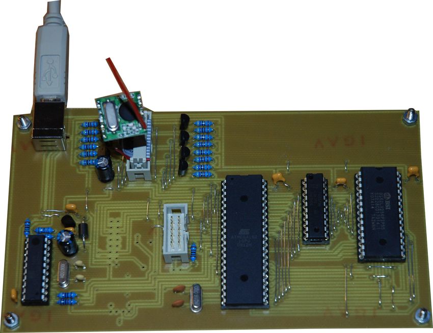
162.3. Printed Circuit Board
Figure 2.4. 2nd revision PCB layout
In order to able to set up future mesh nodes a reproducible hardware design had to
designed. The goal was to be able to produce many mesh nodes and to be able to equip
a whole laboratory. One possibility is to manually wire each mesh node. Due to the
complexity of the schematic this solution was not acceptable. The author decided to
design a printed circuit board (PCB) in order to be able to produce new mesh nodes
quickly. The following design requirements were established by the author:
• One sided PCB: The PCB was aimed to be manufactured in an uncomplicated
environment. Two-sided PCBs allow minimizing the physical size of the device
but for research this is not an important requirement. On the other hand two-
sided PCBs require additional effort. Through-holes have to be manufactured and
eventually the upper side of the PCB has to be laminated in order to prevent
shorts.
• Non-SMD parts: The author explicitly avoided SMD parts. The goal was to
17be able to solder the parts manually with commonly available electronic parts.
The actual design of the PCB (Printed Circuit Board) was performed in three iterative
phases:
• Manually wired prototype : In order to have a proof of concept a first working
prototype was constructed by the author manually. This board was not used for
the final realization but was used in order to test the external RAM as well as
the UART-USB connection.
• 1st revision PCB : A first revision of the PCB was designed and manufactured.
Despite a function node a few design improvements were identified. The trace
count and surface mounting the existing resistors were identified as a further
improvement.
• 2nd revision PCB : The final revision of the PCB was designed in smaller
dimensions and the design flaws from the first revision were corrected.
The final version of the PCB was carefully designed to have a logical and effective
layout of components. Figure 2.5 shows the zones which include the different hardware
modules. The following zones were designed:
18RFM12B radio & Level shifters
USB Power LCD & ISP CPU, Latch & SRAM
Supply PS/2
Keyboard
Figure 2.5. 2nd revision PCB areas
• USB: The USB parts and connectors are being placed in this zone. In order to
have a comfortable connection to the cable the USB connector was placed in the
left upper corner.
• Power supply: Right next to the USB zone the PSU parts are placed.
• RFM12B: The radio modules as well as the level shifters were placed next to
each other.
• ISP: The In-System-Programmer connector was placed next to the CPU in
order to reduce scattering effects.
• CPU, Latch & SRAM: These chips were placed next to each other in order
to reduce the bus trace lengths as much as possible.
19Chapter 3
Software modules and algorithms
3.1. Module architecture
Shell UART Receiver
«userspace» «driver» «userspace»
Network RFM12
«library» «driver»
Watchdog Timer SPI
«daemon» «driver» «driver»
Clock
«daemon»
Figure 3.1. Software modules
The author chose a top-down design approach for the software part of the thesis im-
plementation. This approach consists the following steps:
1. Design a general architecture and identify the necessary software parts (modules)
which need to be connected together.
202. Research the necessary abstractions how the plumbing and inner interoperability
actually should work.
3. Research the necessary algorithms for the final implementation.
The following chapters reflect the above described approach. Figure 3.1 shows the
general module architecture of the thesis implementation. First the following module
stereotypes were identified for the complete software stack:
• Userspace modules: Act like regular "programs". They interact with the user,
retrieve user input and generate user output.
• Driver modules: Provide the necessary abstractions and APIs to external or
CPU internal hardware.
• Daemon modules: These modules are similar to userspace modules but run in
the background only. They do not interact with the user.
• Library modules: Implement APIs and provide those to userspace or daemon
modules.
Afterwards the following concrete modules were identified and implemented by the
author:
1. UART «driver»: This driver module is responsible for the UART interface. It
implements an optimized UART access using ring buffers.
2. SPI «driver»: This driver provides the API to access the serial peripheral
interface.
3. RFM12 «driver»: Implements the API to access the RFM12 hardware module.
It uses the SPI driver module.
4. Timer «driver»: This driver provides the API and callbacks for timer services.
5. Network «library»: This libray module provides the complete network stack
API to userspace modules.
6. Watchdog «daemon»: This daemon updates the watchdog timer of the CPU.
21Furthermore it provides an API in order to reset the CPU manually and add an
error stack information stored in the EEPROM.
7. Clock «daemon»: This daemon is responsible to measure the current time. It
uses the timer driver module.
8. Shell «userspace»: This userspace module is responsible for receiving com-
mands from the serial UART driver, executing commands and printing the result
back.
9. Receiver «userspace»: This userspace module prints out received messages
using the UART driver module.
3.2. Module orchestration
Designing a software system that executes on embedded micro-controllers implies a lot
of challenges when many software modules are involved and complexity grows. The
conceptually defined modules must be somehow implemented. If the micro-controller
lacks an operating system then there is no possibility of using provided abstractions and
APIs for module orchestration and execution. Another challenge are limited hardware
resources which prevent the deployment of many existing operating system kernels.
Basically there are two types of execution models which can be implemented in micro-
controllers:
Module 1
Module 2
Module n
Figure 3.2. Sequential execution model
221. Sequential execution model: This type sequentially executes all modules
inside an infinite main loop starting from the first module until the last one.
Once the last module ends the execution starts again from the first module.
Module 1 Module 2 Module n
Figure 3.3. Concurrent execution model
2. Concurrent execution model: This type executes modules concurrently. In-
stead of having an infinite main loop that iterates sequentially over all modules
the main function only initializes and launches concurrent modules.
3.2.1. Sequential execution
This model does not necessarily needs operating system support or frameworks. It can
be simply implemented as a sequence of function calls inside an infinite loop as shown
in algorithm 1.
Algorithm 1 Sequential model algorithm
while true do
module1
module2
...
modulen
end while
There is one challenge that comes with this type of execution model. That is that only
one module can execute at a time due to its sequential nature. If a module i.e. waits
for an external resource to provide data it must not block the execution of the main
23loop until the external resources becomes ready. This would prevent the execution of
the other modules. The classic solution to this problem is the introduction of states
in modules. Module states can be implemented as classical Finite State Machines
[6].
If we take the example from above about waiting for external resources a finite state
machine for modules can be modeled as shown in figure 3.4.
1
Waiting
Resource available Processing finished
2
Processing
Figure 3.4. State Machine for a module
State machine models can be implemented using if or case statements which is shown
in algorithm 2. The nice side effect of a state machine based implementation is the
non-blocking nature of the module execution. Take for instance the execution of state 1
"Waiting" as shown in figure 3.4. The CPU only needs to execute as many instructions
as are necessary to check if the awaited resource is available. If the resource is not
available the execution returns to the main loop and the next module (together with
its state machine) is being executed.
24Algorithm 2 State machine algorithm
if state is WAITING then
if resource is available then
set state to PROCESSING
else
exit module
end if
else if state is PROCESSING then
process data
set state to WAITING
end if
This implementation emulates a concurrent execution of modules. The context switch
between module executions is being done by the modules themselves (using self-
interruption) and no external scheduler is involved. This form of concurrent behavior
can therefore be described as a non-preemptive or cooperative multi-tasking between
modules. The implementation outlined in [2] heavily used the described state machine
algorithm as shown in listing 3.1.
Listing 3.1. main loop routine [2]
382 while (0 x01 )
383 {
384 if ( uartInterrupt == ON ) // got a character from RS232
385 + - - - - 44 lines :
429
430
431 // --- RECEIVE A DATAGRAM ---
432
433 else if (( datagramReceived = datagramReceive (...))
&& netState > 0)
434 + - - - -182 lines :
616
617
25618 else if ( helloTime ) // prepare periodic Hello message
619 + - - - - 19 lines :
638
639
640
641 // --- SEND A DATAGRAM ---
642
643 if ( datagramReady && netState > 0)
644 + - - - - 8 lines :
652
653 }
A couple of problems arise from the existing implementation. First of all listing 3.1
reveals the following modules:
• UART Module
• Datagram Receiver Module
• Hello Message Sender Module
• Datagram Sender Module
Which module is being executed depends on the state of the main module being repre-
sented by the main function. The state of the main module on the other hand depends
directly from the state of the submodules. The main module therefore acts more like
a controller of the submodules and takes away the responsibility of the submodule’s
state management. Furthermore the main function is very long and complex (271 lines
of code). Therefore the following goals were defined by the author:
• Clear separation of responsibilities between the main loop and the concurrently
running modules.
• Simplification of the main loop implementation.
Listing 3.2 shows the new implementation of the main loop. The new implementation
makes it very clear which modules are being executed sequentially. Furthermore the
26main function does not act as a controller but rather leaves the state management in
the module’s responsibility.
Listing 3.2. main function implementation
95 while ( true ) {
96 shell ();
97 batman_thread ();
98 rx_thread ();
99 uart_tx_thread ();
100 watchdog ();
101 timer_thread ();
102 }
The next question was how to implement the actual concurrently running modules.
One possibility was to reuse the methodology as implemented in [2] and use state
machine based implementations. There is a problem though in state machine based
implementations and that is the rapidly growing complexity. This problem is called
"state explosion problem" and has even a exponential behavior as shown in [7]. The
equation 3.1 shows that the number of states is dependent on the number of program
locations, the number of used variables and their dimensions.
Y
#states = |#locations| · |dom(x)| (3.1)
variable x
where
#states = count of states
#locations = count of program locations
|dom(x)| = the domain of variable x
This equation shows that for instance a program having 10 locations and only 3 boolean
variables already has 80 different states. Although this equation might not apply ex-
actly to state machine based implementations it underlines the practical experience of
27big state-machine based implementations. The alternative to state-machine based ap-
plications are thread or process based implementations using the concurrent execution
model as shown below.
3.2.2. Concurrent execution
This model requires support from an existing operating system. An existing framework
or API provides the necessary abstraction to create new concurrent modules. Each
module runs in isolation and can have its own main loop or terminate immediately. In
terms of operating systems two abstractions are widely used for concurrently running
software modules:
• Processes: Processes are usually considered as separately concurrently running
programs. Usually each process owns its own memory context and communi-
cation with other processes happens through abstractions like pipes or shared
memory.
• Threads: Threads are concurrently running code parts from the same program.
The initial program is considered to run in its own "main thread". Other threads
can be started from the main thread. Threads also do run in isolation to each
other. Each thread has its own stack. Communication with other threads hap-
pens through shared memory provided by static data or the heap.
Processes as well as threads are widely known concepts in classical desktop operating
systems. In the area of embedded micro-controllers these concepts also are implemented
in many different embedded operating systems like FreeRTOS, TinyOS, Atomthreads,
Nut/OS or BeRTOS.
The above solutions have chosen different names for threads or processes (some call
them "tasks") but essentially they all share the same concept of the concurrent execu-
tion model and will be referred to as concurrent modules from now on. Algorithm 3
shows the pseudo-code that initializes concurrent modules. One can see that in contrast
to the sequential execution model the main loop actually does nothing.
28Algorithm 3 Concurrent model initialization
start module1
start module2
...
start modulen
while true do
// no operation
end while
But how does a context switch happen between concurrent modules? Two methodolo-
gies exist:
• Cooperative: The concurrent modules by themselves return the control to a
scheduler which then delegates the control to a different module. Which concur-
rent module gets control is often based on priorities which are controlled by the
scheduler.
• Preemptive: Here the concurrent modules do not have control about how and
when they get interrupted. It can happen anytime during the execution. Again
the context switch between concurrent modules is often handled using priorities
in the scheduler.
Nearly all existing solutions have one feature in common. That is that every thread
has its own separate stack memory space. This is necessary in order to be able to
run the same block of code (for instance a function) in multiple thread instances. On
the other hand threads are being executed in the same memory context so sharing
data between threads is possible by using the heap or static memory. All of the above
mentioned frameworks provide common abstractions which are needed in thread based
implementations:
• Semaphores
• Mutexes
29• Yielding
In contrast to state machine based or sequential based concurrency thread based im-
plementation can be expressed in very linear algorithms using the above mentioned
abstractions. Take for instance the state-machine based algorithm 2. This could be
translated into a linear thread-based algorithm as shown in 4.
Algorithm 4 Thread based algorithm
while true do
wait for resource mutex
process data
release resource mutex
end while
One can easily see that the thread-based algorithm 4 is much more expressive than the
state-machine based algorithm 2.
Together with the necessity of having a scheduler these solutions can be considered
as heavy-weight. The scheduler consumes additional CPU cycles and the separate
stack memory space per thread consumes additional memory which is very scarce in
embedded micro-controller systems.
Although usually a concurrent execution model must be provided in form of an API
or an existing kernel there is one exception in the context embedded micro-controllers
and that are ISRs (Interrupt Service Routines). Interrupt service routines behave like
preemptive concurrent modules with highest priority.
30Main program ISR
Figure 3.5. Illustration of an Interrupt Service Routine
The ISR interrupts the main program at any time when an external resource triggers
an event and executes the service routine. The scheduler in this case is the CPU itself.
There is one caveat with ISRs. When one ISR is being executed no other ISR can be
triggered. Therefore it is being considered best practice not to perform intense and
long running operations in ISRs.
3.2.3. Conclusion
For the implementation of this thesis the following conclusions were drawn:
• Existing solutions supporting the concurrent execution model were considered too
heavy-weight for this type of application. Although 32KB of RAM are available
the purpose is the support of route storage and network support.
• A sequential execution model was favored instead of the concurrent execution
model. On the other hand thread-like linear algorithms are definitely favored
instead of state machine based implementations which could lead to a state ex-
plosion.
One framework exists which implements the sequential execution model but providing
a linear thread-like API being called Protothreads as described in [8]. It is implemented
using C macros and expands to switch statements (or to goto statements if the GCC
31compiler is being used). Instead of consuming a complete stack per thread the pro-
tothread implementation uses only two bytes per (proto)thread. Protothreads actually
are stackless and variables initialized on the stack of a protothread function will stay
initialized only during the very first call of the protothread.
Algorithm 5 Simple linear algorithm
while true do
wait until timer expired
process data
end while
Algorithm 5 shows a very simple linear use case where it waits for an external resource.
In this case it waits for the expiration of an external timer by merely watching the
timer’s state. Since this is a read-only operation no explicit mutual exclusion is needed.
This algorithm expressed as a protothread implementation is shown in listing 3.3.
Listing 3.3. linear protothread implementation
19 PT_THREAD ( test ( void ))
20 {
21 PT_BEGIN (& pt );
22 PT_WAIT_UNTIL (& pt , timer_ready ());
23 process_data ();
24 PT_END (& pt );
25 }
The implementation of the algorithm is self-describing and corresponds to the APIs
known from the concurrent execution model. The expanded version of the listing after
the preprocessor stage is seen in 3.4.
Listing 3.4. expanded linear protothread implementation
char
test ( void )
{
// PT_BEGIN
switch ((& pt ) - > lc ) {
32case 0:
// PT_WAIT_UNTIL
do {
(& pt ) - > lc = 22;
case 22:
if (!( timer_ready ())) {
return 0;
}
} while (0);
process_data ();
// PT_END
};
(& pt ) - > lc = 0;
return 3;
}
The expanded version after the preprocessor stage of the implementation looks much
more like a state machine based implementation from the sequential execution model.
It uses a clever trick called loop unrolling [9] which breaks ups the while statement
using the switch statement. This technique is also known as Duff’s device as described
in [10]. Unfortunately this implementation has one drawback. One cannot (obviously)
use switch statements in protothreads. A slightly more efficient implementation using
GCC labels circumvents this. Since the context switch is managed by the concurrent
modules themselves the behavior can be classified as cooperative multitasking.
Due to the lightweight nature of protothreads and the possibility to express algorithms
in a linear thread-like fashion this framework was chosen by the author for the imple-
mentation.
33Listing 3.5. Sender route for the UART module [2]
void rsSend ( uint8_t data )
{
while ( !( UCSRA & (1 < < UDRE )));
UDR = data ;
}
3.3. Ring Buffers
The implementation as outlined in [2] used the UART interface in order to communicate
with the user and to inform about incoming packets, changes to routes, etc.. As already
analyzed in the previous chapter a state machine based sequential concurrent model
was used to implement the UART module. There exists one problem with the current
implementation.
Listing 3.5 shows that the algorithm examines the UCSRA (USART Control and Status
Register A) and blocks infinitely until the UDRE (USART Data Register Empty) bit
becomes zero. The execution of all other concurrent modules and the main loop will
be blocked until the UART becomes ready to accept data. In this time period no data
can be received from the radio. The above mentioned implementation uses the same
function for sending strings via the UART interface. For sending the string "hello" via
the UART with a speed of 19.2kbps the main loop will be physically blocked for 2.5
milliseconds. In order to improve the implementation the author wanted to accomplish
the following goals:
• Refactoring to a non-blocking operation.
• Migration to a concurrent execution model using protothreads.
The ATmega162 micro-processor offers the following ISRs for receiving and sending
data via the UART [11]:
• SIG_USART_RECV: Is being invoked, when the UDR register contains a
new byte received from the UART.
• SIG_USART_DATA: Is being invoked, when the UDR register is ready to
34be filled with a byte to be transmitted via the UART.
So we have the possibility to send or receive data asynchronously from the main loop in
the context of a concurrent execution model by using ISRs. Filling the UDR or reading
the UDR in the main loop (and thus blocking it) is actually not necessary at all. The
main loop can communicate with the ISRs through a receiving and transmitting queue
buffer where it writes data to the transmitting queue and reads data from the receiving
queue.
Using this sort of communication is known as the "producer-consumer problem". It
can be implemented using a FIFO buffer. The Linux kernel ([12] chapter 5.7.1) as
well as (embedded) DSP micro-controllers [13] use a very elegant FIFO-algorithm by
providing a lock-free buffer being called "circular buffer" or "ring buffer".
End Start
Head Tail
Figure 3.6. Illustration of a ring buffer
Figure 3.6 shows the basic principle of the algorithm. A circular buffer is defined by
the following four pointers:
• Start: This pointer defines the beginning of the buffer in memory. This pointer
is static.
• End: This pointer defines the end of the buffer in memory. It can also be
expressed as the maximum length of the buffer. This pointer is static.
• Head: The head pointer is being changed dynamically by the producer. When-
ever the producer wants to write data in the buffer the head pointer is increased
35and the corresponding memory filled. If the head points to the same address as
the tail pointer the buffer is full or empty.
• Tail: The tail pointer is being changed dynamically by the consumer. Whenever
the consumer wants to read data from the buffer the tail pointer is increased and
the corresponding memory cleared. If the tail points to the same address as the
head pointer the buffer is full or empty.
In order to distinguish whether the buffer is full or empty an additional size variable
was implemented. The biggest advantage of the presented algorithm is the possibility
to write and read data in a lock-free fashion. A consumer thread does not need to wait
for a mutual exclusion on the buffer since the consumer thread is the only instance ma-
nipulating the tail pointer. The same applies for the producer being the only instance
manipulating the head pointer.
The complete listing of the ring-buffer implementation can be seen in appendix A in
the file src/ringbuf.c. There are two functions provided:
• ringbuf_add: This function is being called by the producer. The function
immediately returns true if a byte could be written to the the buffer or false if
the buffer is full.
• ringbuf_remove: This function is being called by the consumer. The function
immediately returns true if a byte could read from the buffer or false if the
buffer is empty.
The important nature of the above mentioned functions is that they are non-blocking
because they return immediately. These functions could therefore be called from pro-
tothreads. A producer protothread running in the context of the main loop can write
data like presented in listing 3.6. The consumer of this data is the SIG_USART_DATA
ISR as presented in listing 3.7.
Listing 3.6. Producer writing data
PT_THREAD ( producer ( uint8_t data ))
{
36PT_BEGIN (& pt );
PT_WAIT_UNTIL (& pt , ringbuf_add ( buf , data ));
PT_END (& pt );
}
Listing 3.7. Consumer reading data
ISR ( SIG_USART_DATA )
{
uint8_t c ;
if ( ringbuf_remove ( buf , & c )) {
UDR = c ;
}
}
Instead of physically blocking the algorithm expressed in listing 3.6 only logically blocks
the protothread. If the buffer is full a context-switch back to the main loop is performed.
The main loop sequentially executes all other concurrent modules and returns to the
protothread which then again tries to add data into the ring buffer.
3.4. Half-Duplex Radio Access
3.4.1. Problem definition
The implementation outlined in [2] used an identical (physically) blocking implemen-
tation in order to send or receive data via the RFM12B hardware module. Listing 3.8
shows the algorithm used for sending data.
Listing 3.8. Sender routine for the RFM12B hardware module [2]
void rfTx ( uint8_t data )
{
while ( WAIT_NIRQ_LOW ());
rfCmd (0 xB800 + data );
}
37This implementation physically blocks the main loop the same way as the UART
algorithm shown in listing 3.5. In this case the algorithm does not wait for the status
of an internal register to send data but rather waits for the external nIRQ pin from
the RFM12B hardware module to go low. The official "RF12B programming guide"
[14] also proposes a physically blocking algorithm.
The author wanted to improve the algorithm in a similar fashion as the UART algo-
rithm. The nIRQ pin of the RFM12B was connected to the INT0 pin of the ATmega162
micro-processor allowing to execute the SIG_INTERRUPT0 interrupt service routine
asynchronously. But it turned out that the implementation could not be reused at
all. The RFM12B radio hardware imposes the following algorithmic challenges for the
driver implementation:
• Single interrupt request for multiple events: The RFM12 radio module
uses only one nIRQ pin in order to generate an interrupt for the following events
[15]:
– The TX register is ready to receive the next byte (RGIT)
– The RX FIFO has received the preprogrammed amount of bits (FFIT)
The state management has to be implemented in software otherwise the current
state of operation (sending or receiving) is undefined.
• Half-Duplex operation: The RFM12 radio module only allows either to receive
or to send data at a time but not simultaneously.
The author abstracted the operation of the RFM12B driver algorithm as a
(proto)thread. Interestingly enough the thread has a state modeled as a state ma-
chine depending whether it receives or sends data. The following states are valid:
• RX: This is the receiving state. The thread (logically) blocks until a complete
packet has been received. Whether a packet is complete or not depends on the
upper network stack layers.
• TX: This is the sending state. The thread (logically) blocks until a complete
38packet has been sent. Again the upper network stack layers decide whether the
transmission is complete or not.
The abstract algorithm is shown in 6. Receiving data is non-deterministic. A packet
can arrive at any time and thus the invocation of the SIG_INTERRUPT0 interrupt
service routine. Therefore the algorithm sets the RX state as the default state for the
radio thread. After receiving the whole packet the driver has to signal the receiver
thread that it can process the packet.
Algorithm 6 RFM12B driver thread algorithm
while true do
if state is RX then
receive data
signal completion to receiver thread
else if state is TX then
send data
signal completion to sender thread
end if
set state to RX
end while
Sending data on the other hand is deterministic. When a user hits the Enter key via
the UART module a packet can be constructed. A sender thread has to inform the
radio driver thread to change its state to TX and wait until the packet has been fully
transmitted. The author realized that this is a concurrency problem between three
threads and a single resource:
• Sender Thread: The sender thread running inside the main loop wants to
acquire the control over the radio module until the transmission of a packet is
complete.
• Radio Thread (ISR): The radio thread being executed in the ISR also wants to
acquire the control over the radio module until the packet reception is complete
39if it is in the RX state or until the packet transmission is complete if it is in the
TX state.
• Receiver Thread: The receiver thread running inside the main loop wants
to acquire the control over the radio module until the reception of a packet is
complete.
• Single resource: The external resource in this case is the radio module. Only
one thread at a time can own the radio hardware resource.
The question is who controls the state of the radio thread and who and when acquires
and releases the lock on the single resource (the radio module). The author decided that
this is rather a complicated algorithm which needs further research and investigation.
The solution to this problem will be presented in the next two chapters.
3.4.2. Petri net model
Until now the challenge was to research an appropriate implementation algorithm for
the (quasi-) parallel execution of modules. Now the author has a new challenge to solve
that a single resource had to be shared between many concurrently executing modules.
The author wanted to find a way to model and simulate an algorithm before actually
implementing it. The purpose of the model is to validate the correct behavior of the
complete algorithm. The most common models for parallel processing are:
• Process calculus
• Actor model
• Petri nets
The author chose the petri net model as this allowed for a visual modelling of the
concurrent algorithm. Many different formal definitions for petri nets exists. According
to Peterson [16] a petri net is composed of a set of:
• A set of Places P = {p1 , p2 , . . . pn }.
40• A set of Transitions T = {t1 , t2 , . . . tm }.
• An input function I who maps from a transition tj to a collection of input places
I(tj ) = {p0 , p1 , . . . , pi }.
• An output function O who maps from a transition tj to a collection of output
places O(tj ) = {p0 , p1 , . . . , po }.
Using the set theory the petri net structure can be expressed as a graph G containing
vertices V and connecting arcs A. A vertex can either be a place pn or a transition
tm . An arch can connect a tuple of two vertices with the restriction that the source
and destination are different types of vertices. Thus arcs cannot connect two places
nor two transitions. These rules can be expressed mathematically as follows:
G = (V, A)
V = {v1 , v2 , . . . vn }
A = {a1 , a2 , . . . an }
V =P ∪T
∅=P ∩T
ai = (vj , vk ) where vj ∈ P and vk ∈ T
or vj ∈ T and vk ∈ P
The petri net graph itself has the following properties:
• Bipartite: The graph consists of vertices (places or transitions) and arcs con-
necting them.
• Directed: Directed arcs connect places and transitions.
• Multigraph: Multiple arcs from one node of the graph to another are allowed.
41Until now only the static properties of a petri net were defined. The dynamic behavior
of a petri net can be modelled using marking. A marked petri net contains one or more
tokens which can only reside inside places (not transitions). Peterson [16] expresses the
marking of a petri net as a vector µ = µ1 , µ2 , . . . , µn which stores the number of tokens
for each place pi in a petri net. The marking of a petri net is not constant through the
life-cycle but rather changes over time. The change of a marking will be expressed as
a token movement from a place "A" pa to a place "B" pb .
This abstraction allows to animate the change of petri net marking by moving tokens
from one place to another. The following rules are valid for the petri nets presented in
this thesis. They were mostly taken from Peterson [16] and a few rules were added by
the author:
• A token always travels "through" a transition and stops "in" a place.
• In a "limited" place only up to n tokens can reside concurrently.
• If a place containing a token is connected as an input to a transition it is called
an "enabled transition".
• All places connected as an output to an enabled transition will receive a token.
• A token having no input places is always enabled. It can emit any number of
tokens at any time.
• An enabled transition having no output places can always receive a token which
disappears.
• An "immediate" token has to be disabled immediately if enabled.
The author used the following symbols in this thesis:
42A place pi
A limited place pi . Stores up to n tokens.
n
A transition ti
imm An immediate transition ti
An enabled transition
A token
Figure 3.7. Petri net symbols
But how can this abstraction be used to model concurrency? The key aspect is that a
marking of a petri net at a discrete point of time simply expresses the current state of
the complete system. The location of a token (the place it currently resides in) defines
the system state. A concurrently running system includes multiple states, one for each
concurrently running module as was shown in the previous chapter. Thus a concurrent
system includes multiple locations in which tokens can reside.
Regarding the initial problem we can as an example define two concurrently running
modules which have to share a common resource. The following states can be de-
fined:
• Module 1 state: The location of this token abstracts the current state of the
first module.
• Module 2 state: The location of this token abstracts the current state of the
second module.
• Lock state: The two modules both have critical section of code which must run
mutually exclusive because they share a common resource. A lock (mutex) has
to be introduced. The mutex token location represents the state of the mutex
lock.
The common petri net model for mutual exclusion as proposed by Peterson [16] can
be seen in figure 3.8. It was used by the author as the basis for the development of its
own algorithm.
43Module 1 Module 2
Critical
Section
Mutex
Figure 3.8. Mutual exclusion Peterson petri net model
3.4.3. RFM12 driver petri net model
Sender thread
rfm12_lock
wait(
mutex) 1
wait(tx) Radio thread (ISR)
1
next
TX imm
end
imm
nIRQ
signal(mutex) 1
imm
wait(rx)
RX imm
next
end
imm
1
Receiver thread
Figure 3.9. Half duplex algorithm modeled as a petri net
The final algorithm for the RFM12 driver is shown in figure 3.9. It shows the three
above mentioned threads (sender, receiver and radio ISR) in the initial states:
• Sender thread: The sender thread includes an always enabled transition which
emits a token whenever the user prompts to send a message. When this happens
44it waits until it can acquire the control over the radio module in order to send a
complete packet.
• Receiver thread: The receiver thread by default always logically blocks in a
waiting state until a packet reception is complete.
• Radio thread: The radio thread is in the RX (or idle) state by default. All
transitions in the radio thread are immediate transitions. This is because the
interrupt service routine itself cannot be interrupted which is a constraint defined
by the hardware of the used CPU. A context switch to other threads therefore
can only then happen when there are no enabled transitions in the ISR.
The next two chapters explain the two major use cases "Data reception" and "Data
transmission" by describing how the petri net model (and thus the algorithm) behaves.
The petri net behavior is used to validate the correctness of the algorithm:
Data reception
Whenever the radio module detects a valid sync pattern it will fill data into its FIFO
buffer. When the reception of one byte is complete the radio hardware pulls the nIRQ
pin low triggering the ISR. The model shown in figure 3.10 shows this behavior as an
infinitely enabled transition labeled as "nIRQ" which can fire at any non-deterministic
time. The following figure 3.10 and the corresponding events describe the behavior
when a new byte is received by the radio.
45Radio thread (ISR)
next
imm
end
imm
1.
2. 2. nIRQ
signal(mutex)
imm
wait(rx) 3.
RX imm
next
end
imm
1
Receiver thread
Figure 3.10. nIRQ triggers reception
1. The nIRQ transition fires the ISR. An interrupt occurs caused by the radio mod-
ule.
2. The radio thread being in the RX state by default tries to acquire the lock (mutex)
on the radio and succeeds. Since the mutex is free the interrupt source must be
caused by the reception of a byte.
3. The radio thread can begin its critical section by taking the received byte and
delegating it to the upper network layers. The radio thread stays in the RX state
and blocks the radio by not releasing the mutex.
Since the radio module has acquired the lock on the radio a sender thread will have to
wait until the mutex will be released. All following nIRQ interrupt sources therefore
also must be caused by a reception of a next byte which is shown in figure 3.11.
46Radio thread (ISR)
next
imm
end
imm
1.
nIRQ
signal(mutex)
imm
wait(rx) 2. 2.
RX imm
next
end 3.
imm
1
Receiver thread
Figure 3.11. Next byte reception
1. The nIRQ transition fires the ISR. An interrupt occurs caused by the radio mod-
ule.
2. The radio thread is in the RX state and already acquired the lock (mutex) on the
radio. It is ready to receive the next byte and delegates it to the upper network
layers.
3. The upper network layers did not indicate that the reception is complete so the
radio thread stays in the RX state.
Still no sender thread will be able to acquire the mutex lock. The above described
reception of bytes happen until the upper network layers detect the end of a frame or
packet which is described in figure 3.12.
47Radio thread (ISR)
next
imm
end
imm
1.
nIRQ
signal(mutex)
imm
wait(rx) 2.
5. 4. RX imm
3. next
end
imm
5. 4. 4. 1 3.
Receiver thread
Figure 3.12. Final byte reception
1. The nIRQ transition fires the ISR. An interrupt occurs caused by the radio mod-
ule.
2. The upper network layers decide that the reception is complete. The mutex on
the radio can be released.
3. After releasing the mutex the receiver thread is signalled by the radio thread
that the reception of a packet is complete. The signal itself is emitted by upper
network layers who need to wait for the receiver thread to process the incoming
packet.
Note that this is a limited place (currently with the limit of one token). The
maximum number of token corresponds to the maximum number of packets which
have to be buffered by the network stack. If the receiver thread is too slow to
process incoming packets all further incoming packets will be dropped.
4. The receiver thread now changes its state. From a waiting state it switches to a
processing state where it processes the received packet and i.e. displays it on the
console.
5. The receiver thread finally switches back to a waiting state in order for the next
packet to arrive.
48Data transmission
The data transmission in contrast to data reception is triggered by the sender thread.
Thus figure 3.13 shows an infinitely enabled transition in the sender thread which
triggers a token (a packet to be sent) whenever the prompts a new send command.
The following figure 3.13 describes the behavior when a new packet is sent by the
sender thread.
Sender thread
rfm12_lock
1.
wait(
mutex) 3.
1
2.
wait(tx) Radio thread (ISR)
3. 1
next
TX imm
end
2. imm
nIRQ
signal(mutex) 1
imm
imm
next
end
imm
Figure 3.13. Sender thread triggers transmission
1. The sender thread tries to send a new packet by changing its state to a mutex
waiting state. It waits for the mutex to become free in order to acquire the lock
on the radio module.
2. If the radio module becomes free the mutex can be acquired. The radio module
transmitter hardware and the radio module transmitter FIFO is enabled.
3. Because the sender thread took over control it resets the radio driver thread to
the new state TX. Afterwards the sender thread puts itself into a waiting state
until the packet transmission is complete.
49You can also read