Gender, Electoral Incentives, and Crisis Response: Evidence from Brazilian Mayors - UCLA ...
←
→
Page content transcription
If your browser does not render page correctly, please read the page content below
Gender, Electoral Incentives, and Crisis Response:
                         Evidence from Brazilian Mayors∗

                      Juan Pablo Chauvin1 and Clemence Tricaud2
                               1
                                   Inter-American Development Bank
                                     2
                                       UCLA Anderson and CEPR

                                                July, 2021

                                                  Abstract
           While there is evidence of gender differences in policy preferences and electoral strategic
       behaviors, less is known about how these differences play out during crises. We use a close
       election RD design to compare the performance of female- and male-led Brazilian municipalities
       during the COVID-19 pandemic. We find that having a female mayor led to more deaths per
       capita early in the first wave of the pandemic – a period characterized by great uncertainty
       about the severity of the disease and the effectiveness of containment policies. In contrast,
       having a female mayor led to fewer deaths per capita early in the second wave – a period where
       this uncertainty was reduced, and when the 2020 mayoral election took place. Consistent with
       the evolution of deaths, we find that female mayors were less likely to implement commerce
       restrictions at the beginning of the period, while they became more likely to do so at the end. We
       also show that the second-wave effect coincides with a lower tendency of the population in male-
       led municipalities to stay at home around election day. Both the first and second wave effects
       are driven by municipalities whose mayors were not term limited, and thus allowed to run for
       re-election. These findings suggest that the gender differences we observe stem from female
       and male mayors reacting differently to electoral incentives. While electorally motivated female
       mayors were more likely to delay restrictive policies at the beginning, electorally motivated
       male mayors were more likely to open-up the municipality closer to the election.

   ∗
     Chauvin: juancha@iadb.org, Tricaud: clemence.tricaud@anderson.ucla.edu. We thank Samuel Berlinski,
Vincent Pons, Razvan Vlaicu, Romain Wacziarg, Melanie Wasserman, and seminar participants at the IADB-
RES Early Research and the Urban LACEA online seminars for their helpful comments and suggestions.
Nicolás Herrera L., Rafael M. Rubião, Juliana Pinillos, Haydée Svab, and Julio Trecenti provided outstanding
research assistance. The opinions expressed in this publication are those of the author and do not necessarily
reflect the views of the Inter-American Development Bank, its Board of Directors, or the countries they
represent.

                                                       1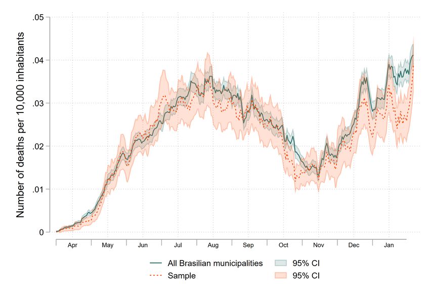
1        Introduction
A large literature documents gender differences in the behavior of elected officials. Com-
pared to male politicians, female politicians have been shown to invest more in certain
public goods such as health and education (Chattopadhyay and Duflo, 2004; Clots-Figueras,
2012; Bhalotra et al., 2014; Funk and Philips, 2019), and to be less likely to engage in corrup-
tion and strategic electoral behaviors (Brollo and Troiano, 2016).1 However, there is still
little evidence on how these differences play out during crises, when high-stake decisions
need to be made hastily and under uncertainty.
        This paper studies gender differences in leaders’ response to the COVID-19 pandemic,
a crisis that posed extraordinary challenges to policymakers all over the world. Focusing
on Brazil – the country with the second-highest COVID-19 death toll in 2020 (Roser et al.,
2021) – we investigate whether female and male mayors handled the crisis differently, and
how it ultimately affected the number of COVID-19 deaths in their municipalities.
        This setting offers several advantages. First, Brazilian municipalities are federal entities,
which implies that mayors can independently choose over which containment policies
to adopt, contrary to many countries where these decisions are taken at the national or
regional level. Second, the large number of Brazilian municipalities allows us to use a
close election design to assess the causal impact of female leadership. Third, we gathered
panel data at the municipal level on the number of COVID-19 deaths, the policies that were
implemented, and the share of residents staying at home. We can thus explore the role
of containment policies and isolation in explaining the differences in COVID-19 mortality
across municipalities and over time.
        A key feature of our setting is that a subset of mayors faced electoral incentives during
the crisis. The 2020 municipal election took place on November 15, less than nine months
after the first confirmed infection in the country. In Brazil, mayors are subject to a two-term
limit (Ferraz and Finan, 2011; de Janvry et al., 2012), meaning that only first-time mayors
could run for re-election. By exploiting this variation, we can assess whether the gender
differences we observe are driven by female and male mayors responding differently to
electoral incentives.
        We explore the impact of mayors’ gender over the period going from February 2020 –
    1
    The three first papers study female legislators in India, while the last two look at female mayors in Brazil.
The evidence is less conclusive in high-income countries (Ferreira and Gyourko, 2014; Bagues and Campa,
2021).

                                                       2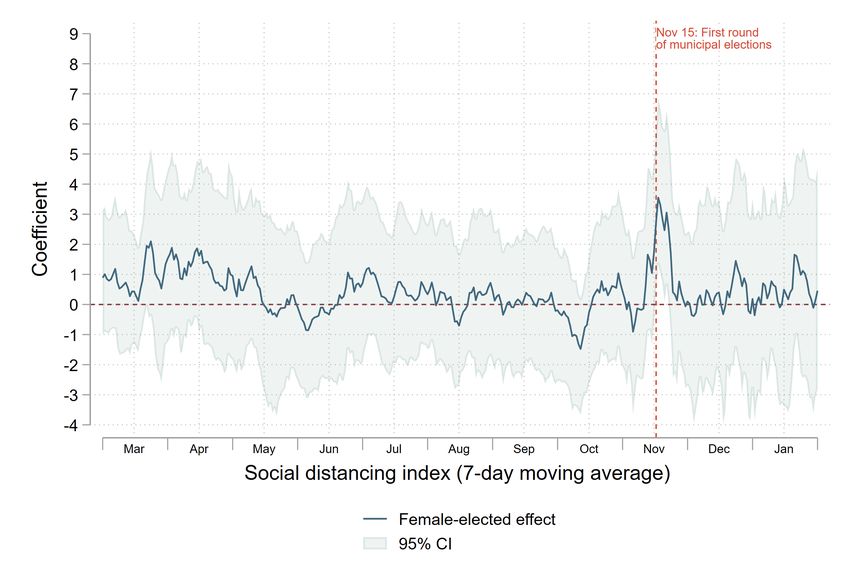
when the first COVID-19 case was detected in the country – to the end of January 2021 –
one month after the mayors elected in November took office. In order to isolate the causal
impact of having a female mayor, we use a Regression Discontinuity Design (RDD) and
compare municipalities where a female candidate barely won against a male candidate
in the 2016 election – the last one before the COVID outbreak – to those where a male
candidate barely won against a female candidate.
       This strategy enables us to compare municipalities that are similar in every aspect,
except in the gender of their mayor. To provide support for the identification strategy, we
show that municipalities are indeed balanced on a large set of socio-demographic and
political characteristics at the threshold. Moreover, we show that barely elected female
and male mayors are similar in terms of incumbency status, age, education, and political
orientation. This suggests that our results capture a gender effect, rather than the impact
of other observable characteristics of the mayor.2
       We first measure the impact of female leadership on the number of COVID-19 deaths
in the municipality. We find that – even though the gender of the mayor did not impact
the time at which municipalities experienced their first COVID-19 fatality – the number of
COVID-19 deaths followed a different trajectory over time in female-led compared to male-
led municipalities. At the beginning of the first wave (April-May 2020), having a female
mayor led to a 0.4 increase in the number of deaths per 10,000 inhabitants, corresponding
to a two-fold increase compared to male-led municipalities. This effect disappeared as
the country entered the peak of the first wave, with female- and male-led municipalities
experiencing a similar number of deaths from June to October 2020. We find a large
female-mayor effect again at the end of the year – at the start of the second wave – but
in a markedly different direction. Between November 2020 and January 2021, female-led
municipalities experienced 1.0 fewer death per 10,000 inhabitants, relative to an average
of 2.4 in male-led municipalities. Overall, these two contrasting effects translate into a
negative but non-significant impact on the cumulative number of COVID-19 deaths as of
January 31, 2021.
       We next explore mayors’ decisions over containment policies to understand what drives
these differences. Using data collected directly from laws and decrees issued by the munic-
ipalities, we find that female and male mayors differ primarily in their use of commerce
restrictions. Consistent with the evolution in the number of deaths, we show that female
   2
    We also show that our results are robust to controlling for municipal-level characteristics, mayors’
characteristics other than gender, and to including state fixed effects.

                                                   3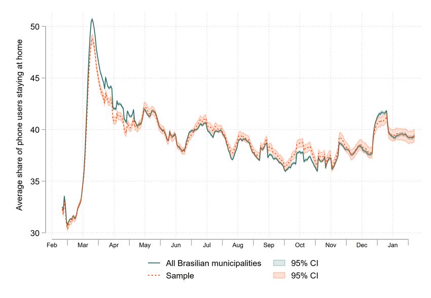
mayors were less likely to close commerce at the beginning of the period, while they be-
came more likely to do so towards the end. First, commerce restrictions were in place
2.5 and 6.5 fewer days in female-led municipalities in March and April 2020, respectively,
corresponding to a 78 and 61 percent decrease relative to male-led municipalities. This
effect is driven by female mayors’ higher likelihood to delay commerce closures, as they
started implementing them 33 days later on average. In contrast, female-led municipal-
ities became significantly more likely to close commerce in the two months leading up
to the November election. Commerce restrictions were in place 7.3 and 7.5 more days in
female-led municipalities in September and October 2020, respectively, corresponding to a
two-fold increase relative to male-led municipalities.
       Additional evidence suggests that the lower number of COVID-19 deaths in female-led
municipalities during the later period is also driven by a higher propensity of residents to
stay at home around election day (November 15).3 Using daily cellphone data, we find
that the share of phone users who stayed at home remained generally the same in female-
and male-led municipalities throughout the period of analysis, except in the days close to
the election.4 Relative to male-led municipalities, the share of residents staying at home in
female-led municipalities was 5 to 7 percent higher the week preceding and following the
election. In particular, it was 11.7 percent higher on November 13, and 17.1 percent higher
on November 14, the last two days before the election in which campaigning was legally
allowed.
       In the last part of the paper, we assess whether these gender differences are driven by
electoral incentives. At the beginning of the first wave of the pandemic, there was great
uncertainty about the severity of the disease and about the effectiveness of containment
policies. Mayors planning to run for re-election could see the electoral risk going both
ways: they could be criticized for not reacting early enough or, instead, for overreacting
if they implemented policies that would prove to be too costly or ineffective by the time
of the election. Female mayors planning to run for re-election may have perceived the
latter risk as higher for their re-election prospects, making them more reluctant to impose
   3
    When referring to election day, we refer to the day of the first round of the 2020 election. Only the largest
municipalities had a second round, and they all end up excluded from our sample of analysis (see Section
3.1).
   4
     The fact that the share of residents staying at home remained the same over almost all the period is
consistent with female- and male-led municipalities differing primarily in their use of commerce restrictions.
Commerce restrictions do not restrict mobility per se, as opposed to other measures such as curfews or
lockdown. They nonetheless promote social distancing and reduce the risk of infections by preventing people
from entering closed spaces.

                                                       4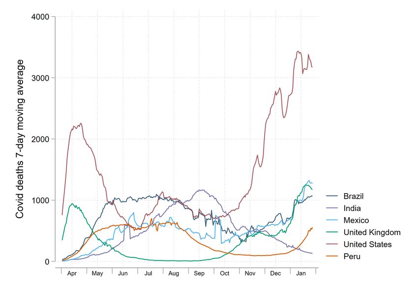
early restrictive measures. If this is the case, our results for this period should be driven by
electorally motivated female mayors.
   In contrast, the period leading to the second wave is characterized by lower uncertainty.
Crucially, this is also when the municipal election took place. Mayors running for re-
election had an incentive to please the electorate before the election, and thus to impose
lower restrictions (Pulejo and Querubín, 2021). Additionally, they could have been inclined
to organize in-person events during the campaign, thus encouraging people to go out,
despite the sanitary recommendations. Male mayors might have been more likely to
respond to such incentives, consistent with evidence showing that they are more likely
to engage in strategic behaviors during the electoral period (Brollo and Troiano, 2016).
If this is the case, our results for the final quarter of 2020 should be driven by electorally
motivated male mayors.
   To test these hypotheses, we split our sample depending on whether the female or
male mayors were term-limited or not. A non-term-limited mayor was allowed to run for
re-election, and thus faced electoral incentives in 2020. Consistent with our predictions,
we find that the positive impact on deaths at the beginning of the first wave is driven by
municipalities where the female mayor could run for re-election, while the negative impact
at the end of the period is driven by municipalities where the male mayor could run for
re-election.
   Overall, our results show that Brazilian female mayors handled the COVID-19 crisis
differently, leading to a different evolution in the number of death over time in female-led
municipalities compared to male-led municipalities. The results appear mainly driven by
the fact that female and male mayors responded differently to political incentives. While
electorally motivated female mayors were more reluctant to impose restrictions early on,
electorally motivated male mayors were more likely to open up the municipality close to
the election.

Contribution to the literature
A growing body of work points to the importance of leaders for economic outcomes (Jones
and Olken, 2005; Besley et al., 2011; Yao and Zhang, 2015; Ottinger and Voigtlander, 2021).
This paper directly contributes to the literature exploring the impact of female leadership.
   In developing countries, several studies find that female representation shapes the
provision of public goods. Exploiting the random assignment of women in Indian village

                                               5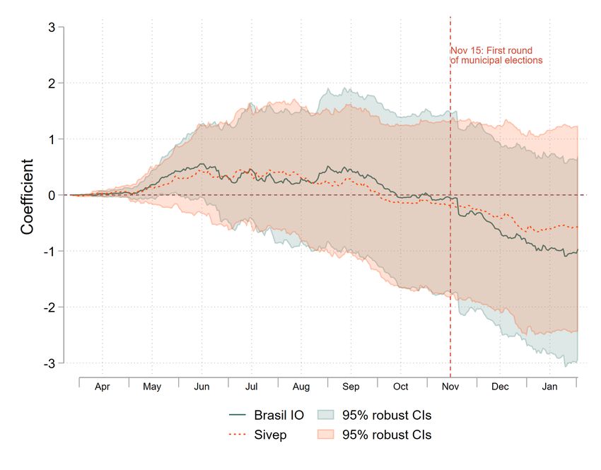
councils, Chattopadhyay and Duflo (2004) show that female representation increases
investments in infrastructure that is relevant to women’s needs. Female politicians also
tend to increase spending in education and health relative to male politicians, as evidenced
by the impact of female state legislators in India (Bhalotra et al., 2014; Clots-Figueras, 2012)
and female mayors in Brazil (Funk and Philips, 2019). The evidence is less conclusive in
high-income countries: while Ferreira and Gyourko (2014) and Bagues and Campa (2021)
find no effect of female representation on the size or composition of public finances in the
US and Spain, Besley and Case (2003) and Lippmann (2021) highlight gender differences
in lawmaking by showing that female legislators are more active on family and children’s
issues.
       This paper makes three important contributions to this literature. First, by studying
leaders’ behavior during the COVID-19 pandemic, we shed light on gender differences in
crisis response, on which there is still little evidence to date.5 Second, while most of the
conclusions drawn about the role of female leaders during the COVID-19 crisis are based
on observational data, the use of a close election design enables us to assess the causal
impact of female leadership.6 Third, by exploiting the term-limit status of Brazilian mayors,
we highlight the role of electoral incentives in shaping female and male mayors’ response
to the crisis.
       We thus also contribute to the large literature investigating the impact of electoral
incentives on policymakers’ behavior. One branch of the literature posits that holding
elections is an effective tool to discipline politicians and align their incentives with voters’
interests (Barro, 1973; Ferejohn, 1986). To test this hypothesis, several papers have exploited
term-limit rules and compared the decisions of politicians who could or could not run for
re-election (Besley and Case, 1995, 2003; Duggan and Martinelli, 2017). In Brazil, consistent
with elections working as a disciplining device, Ferraz and Finan (2011) and de Janvry
et al. (2012) find, respectively, that having a non-term-limited mayor decreases the share of
   5
    One recent paper looking at a crisis context is Eslava (2020). The author finds that that having a female
mayor in Colombia reduces the number of guerilla attacks, an effect argued to come from female politicians’
better negotiation skills.
   6
     A few recent observational studies have used cross-country or cross-state variation to compare the
performance of male and female leaders during the COVID-19 crisis (e.g., Garikipati and Kambhampati
2021; Bosancianu et al. 2020; Sergent and Stajkovic 2020). The results obtained so far are mixed and do not
offer causal interpretation (Profeta, 2020). One exception is a contemporaneously written paper by Bruce
et al. (2021) that looks at the impact of Brazilian mayors’ gender on the overall number of deaths in 2020.
Instead, our paper studies the evolution of deaths, policies and isolation throughout the period, highlighting
contrasting effects at the beginning and end of the year, and stressing the key role of electoral incentives in
explaining gender differences.

                                                      6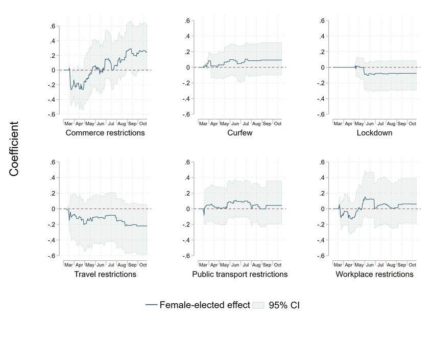
stolen resources and increases the performance of the conditional cash transfer program.
   However, electoral incentives can also lead to sub-optimal outcomes. Knowing that
voters are particularly responsive to the state of the economy close to the election (Healy
and Lenz, 2014), politicians have an incentive to manipulate monetary and fiscal policies
to improve economic performance just before the election, leading to a political business
cycle (Alesina, 1988; Drazen, 2001; Brender and Drazen, 2005; Alesina and Paradisi, 2017).
In the context of the COVID-19 crisis, Pulejo and Querubín (2021) show that incumbents
who could run for re-election implemented less stringent restrictions when the election
was closer in time.
   Our paper bridges the gap between the gender literature and the electoral-incentive
literature, by showing that gender differences in response to the COVID crisis are driven
by the fact that Brazilian female and male mayors reacted differently to electoral incentives.
Our findings at the beginning of the pandemic show that electoral incentives made female
mayors more likely to delay the implementation of restrictive policies. While the underlying
reason explaining this behavior is still an open question, one plausible hypothesis is that
female mayors perceived voters to be more likely to punish them at the ballot box for
implementing harsh policies too soon, rather than for acting too late. This would be
consistent with evidence from the Political Science literature showing that voters view
female and male leaders differently (Eggers et al., 2018; Fox and Lawless, 2011; Dolan, 2014)
and assess their performance differently (Bauer, 2020; Batista Pereira, 2020), in particular
during crises (Lawless, 2004). Meanwhile, our results on the later period show that female
mayors were less likely to open-up the municipality right before the election, in line with
Brollo and Troiano (2016), who find that Brazilian female mayors are less likely to engage
in strategic behavior close to the election.

   The remainder of the paper is organized as follows. Section 2 presents our setting
and the data, and Section 3 describes our sample and empirical strategy. We present the
main results in Section 4, and explore the role of electoral incentives in Section 5. Section 6
concludes.

                                               7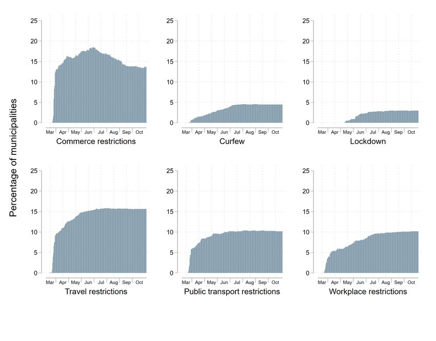
2        Setting and data

2.1       Brazilian local governments and elections
Brazil is divided in 5,570 municipalities, with an average population of around 39,000
residents according to the 2010 census. Municipal governments are the lowest subnational
government tier in the country.7 The constitution recognizes municipalities as "federal
entities", which gives them the status of autonomous governments, with the ability to
independently decide over local policies. Municipalities’ revenues come mainly from
constitutionally-mandated inter-government transfers, followed by user fees and local
property taxes. Municipal governments are in charge of providing public services of local
interest, including water and sanitation, transportation, basic education, and – importantly
for this paper – public health.
        Municipal governments have an executive branch (prefeitura) and a legislative branch
(câmara municipal). The executive branch is presided by mayors who are elected by pop-
ular vote every 4 years, and are subject to a strict two-term limit established by the 1988
constitution. Voter registration and voting is mandatory for adults between the ages of 18
and 70. The electoral rule depends on the municipal population. Municipalities with fewer
than 200,000 inhabitants elect their mayors through plurality rule – where the candidate
with the most votes wins the election – while municipalities with 200,000 inhabitants or
more use a two-round system.
        Our empirical strategy relies on the results of the 2016 municipal election, the last
election before the onset of the COVID-19 pandemic. The term of the mayors elected in
2016 ran from January 1, 2017 through December 31, 2020. The first round of the next local
elections took place in November 15, 2020, and the new mayors took office on January 1,
2021. We define our period of analysis from February 2020 (first registered case in the
country) through the end of January 2021.8
        The 2020 municipal election was originally scheduled on October 4 and postponed to
November 15 due to the COVID-19 health emergency. While basic safety protocols were put
in place at the voting booth (face mask use and availability of hand sanitizers), the election
    7
    The first tier consists of 27 "federative units", made of 26 states and the Federal District. The Federal
District does not contain any municipality; it is divided into administrative regions, including the capital
Brasilia, and in thus excluded from the analysis.
    8
    We include the first month of the new municipal administration as COVID-19 deaths tend to materialize
a few weeks after infection, implying that people that died from the disease in January likely became infected
while the prior mayor was still in office.

                                                      8
took place in person as the previous ones.9 During the electoral campaign leading to the
election, local media reported multiple breaches of sanitary protocols, in particular large
in-person gatherings violating the social distancing recommendations (Tarouco, 2021).
2.2 The COVID-19 pandemic in Brazil
The authorities announced the first confirmed COVID-19 case in Brazil on February 26,
2020, and the first confirmed death three weeks later, on March 17. The disease expanded
exponentially across the country, and so did the death toll. While Brazil registered 201
COVID-19 deaths by the end of March, it reached 6,006 by the end of April, and 28,834 by
the end of May (Roser et al., 2021). At the beginning, the affected cities were primarily
large urban centers located close to international airports, but infections gradually reached
smaller and less connected cities as well as rural areas. Following the news of the first
confirmed death, multiple states and municipal governments declared state of emergency
and some started implementing containment policies such as school and commerce closures,
along with public gathering restrictions.
The period of analysis is characterized by the development of the first wave of infections
(February 2020 - October 2020), and by the beginning of the second wave (November
2020 - January 2021). The first wave in Brazil was one of the deadliest worldwide. After
reporting more than 1,000 deaths per day for the first time on May 19, the country endured
similarly high mortality levels for around three months, longer than in any of the other
high-mortality countries (Figure 1). On June 10, Brazil’s cumulative number of deaths
overcame the number of deaths reported by the U.K., and the nation became the second
country in the world with the most deaths attributed to COVID-19, behind the U.S. The
second wave started in November and proved to be even deadlier than the first. By the end
of the period of analysis, the daily number of deaths had reached similar levels as in the
peak of the first wave, and the country had accumulated over 224,000 deaths in total. It
would go on to reach over 4,000 new deaths per day at its peak, and over half a million
accumulated deaths by June 2021.
9
After consulting a health safety committee, the electoral justice court (TSE) considered online or postal
voting infeasible and decided to stick to in-person voting.
9Figure 1: Daily number of COVID-19 deaths in Brazil and in the other five countries with
the highest mortality (7-day moving average)
Notes: This figure includes the six countries with the highest number of confirmed COVID-19 deaths in the
world as of January 31, 2021. It shows the new confirmed COVID-19 deaths, smoothed using a 7-day moving
average centered in the date for which the figure is reported. Data from Our World in Data, accessed on June
23, 2021.
2.3 Data
We use data on three outcomes of interest – COVID-19 deaths, municipal containment poli-
cies, and the share of people staying at home – in addition to electoral data and municipal
characteristics. Appendix Table A1 provides the definition and source of each variable
used in the paper.
COVID-19 deaths. The data on COVID-19 deaths come from Brasil.io, an open data
platform that collects, cleans, and assembles the COVID-19 information provided by the
state-level health secretaries, and makes it publicly available as a daily municipal-level
panel (Justen, 2021). We focus on confirmed deaths rather than cases. Deaths has been
considered a more reliable measure of the spread of COVID-19 as well as of the spread of
other diseases such as SARS and Ebola (Maugeri et al., 2020; O’Driscoll et al., 2021), as they
are less likely to go unrecorded. We observe the daily number of COVID-19 deaths from
the first registered death on March 17, 2020, until January 31, 2021. We performed quality
10checks to identify potential data errors and outliers and we only found unusual spikes in
a few municipalities located in the state of Mato Grosso. We exclude municipalities part
of this state in one of our robustness check (Appendix F) – representing 3 percent of the
sample –, as well as when presenting the raw data on the number of deaths in Section 3.1.
In addition, we validate our main results using alternative data from the Brazilian
System of Information and Epidemiological Surveillance of Respiratory Infections (SIVEP-
Gripe), a patient-level registry of deaths from severe acute respiratory syndrome (SARS)
that contains data from both public and private hospitals. This dataset is maintained by
the Ministry of Health of Brazil. Both data sources are highly consistent during the period
of analysis, as shown in Appendix F.10
Containment policies. To study mayors’ policy responses, we built a novel policy
dataset based on publicly available municipal legislation documents, following the proce-
dure from Chauvin et al. (2021). We accessed multiple online sources, including municipal
websites and official gazettes, and collected local laws, decrees, and other mandates issued
by the municipal executive branch in response to the COVID-19 crisis. We then extracted
the text of the legal documents, parsed their individual articles, and used them to construct
a daily panel of indicator variables that denote whether the policy was in place in a given
municipality for each day. We consider 10 containment policies, in line with the interna-
tional policy data featured in the Oxford COVID-19 Government Response Tracker (Hale
et al., 2020): commerce, gathering, transport, travel, and workplace restrictions, events
cancellations, school closures, curfews, lockdown and face mask mandates. We were able
to collect those data for 47.8 percent of our sample over the period from March 1 to October
31, 2020. Four of these policies (gathering restrictions, school closures, events cancellations,
and face masks mandates) were implemented by the vast majority of municipalities and
sustained for most of the period of study (Appendix Tables A2 and A3), providing little
variation to identify the effects of interest. We thus focus on the remaining six in our
analysis.
Isolation index. To study the mobility behavior of the population, we use the "Social
10
As discussed in more detail in Chauvin (2021), the study of COVID-19 at the municipal level makes it
challenging to compute the number of deaths using alternative measures. Estimating excess deaths relative
to prior years for a given week, for instance, requires historical mortality data with enough variation in each
calendar week to accurately predict the number of deaths that would be expected without the pandemic. This
is only feasible in highly populated jurisdictions, which is not the case of most of the municipalities in our
sample. Likewise, data from seroprevalence surveys to infer infection rates from the presence of antibodies
are only available for a small set of municipalities, most of which are not in our sample.
11Isolation Index" produced by the private firm InLoco (2021). This index is built using
anonymized data from over 60 million cellphones and it indicates the share of active phone
users who stayed within 450 meters of their residence in a given municipality on a given
day. During the pandemic, the company made a daily municipal-level panel available to
researchers. To protect users’ privacy, the data are not available on days where the number
of active users in the municipality was below a given threshold. Furthermore, the number
of municipalities included in the sample gradually decreased over the second half of 2020,
reflecting a change in the company’s business priorities. For consistency, we focus on a
balanced panel of municipalities for which we have data for every day over our period of
analysis, from February 26, 2020 to January 31, 2021 (29 percent of the sample).
Electoral data. The electoral data for the 2016 elections come from the Brazilian elections
authority (Tribunal Superior Eleitoral, TSE). We also performed several data-quality checks
using alternative sources such as press articles and municipal gazettes. For each candidate
in each municipality, we know her gender, incumbency status, age, education level, party
affiliation, and the number of votes she received. We further classify the 32 parties running
in the election into 4 main political orientations: "left", "center-left", "center-right and
liberals", and "right and Christians".11
Municipalities’ characteristics. We also use a large set of municipal socio-demographic
characteristics to test the validity of our identification strategy and the robustness of our
results to the inclusion of controls. Most of these baseline variables are constructed directly
from the microdata of the 2010 demographic census (the last one before the 2016 elections).
One exception is our measure of density -– the total population living within 1 km of the
average inhabitant of the city – which we compute using 2015 data from the Global Human
Settlement Layer (Schiavina et al., 2019) following De la Roca and Puga (2017)’s method.
We made sure to include variables that have been shown to predict the geographic variation
in COVID-19 deaths, such as population, density, the share of residents above 65 years old,
proximity to internationally-connected airports, the number of nursing home residents,
and household income (Chauvin, 2021).12
11
We use a data driven procedure based on a hierarchical cluster analysis. See Appendix A5 for further
details.
12
The 2010 municipal population is also used to normalize the number of deaths per 10,000 inhabitants.
Between 2010 and our period of analysis, five new municipalities were created from seven parent municipali-
ties. Out of these twelve redistricted municipalities, only one qualified to be part of our sample. We removed
it to ensure time-consistent geographies throughout our analysis.
123 Empirical strategy
3.1 Sample and descriptive statistics
To estimate the causal impact of female leadership, we use a Regression Discontinuity
Design (RDD) and compare municipalities where a female candidate barely won against
a male candidate, to municipalities where a male candidate barely won against a female
candidate. We thus restrict our sample to Brazilian municipalities where the top two
contenders in the 2016 election were one female and one male candidates, accounting for
20.4 percent of all Brazilian municipalities.13
We further exclude municipalities for which their COVID-19 outcomes cannot be directly
linked to their local government’s actions. More precisely, we exclude the 18.6 percent
municipalities that are part of a commuting zone (arranjos populacionais), as defined by
the Brazilian institute of Geography and Statistics (IBGE, 2016). A commuting zone is
made of a group of municipalities which are linked through commuting flows and that
often coordinate on urban services such as transport. Hence, the number of COVID-19
deaths in a municipality part of a commuting zone are likely to be largely affected by the
spread of the virus inside the commuting zone and by the policy choices of its neighbors,
in particular the ones of the central city.14
Our final sample consists of 983 municipalities. As shown in Figure 2, they are evenly
spread out across all Brazilian states, and there is no clear geographical patterns between
municipalities where a female candidate was elected (in blue) and municipalities where a
male candidate was elected (in red).
Table 1 presents descriptive statistics on our sample.15 The first panel includes socio-
demographic characteristics from the 2010 census. The second panel includes political
characteristics based on the first round of the 2016 election.16 Municipalities in our sample
13
We exclude 30 municipalities where the votes of one of the top two candidates were invalidated by
the electoral justice due to irregularities. In 25 of the municipalities in our sample, the election as a whole
was cancelled and a supplementary election took place later on. In these cases, we ignore the results of the
ordinary election and consider the top two candidates in the supplementary one. Our results are robust to
excluding those municipalities (see Appendix F).
14
Arranjos populacionais are similar to urban commuting zones in the US. As an example, Sao Paulo
commuting zone includes 37 municipalities. The spread of COVID-19 in those municipalities was tightly
linked to the policies decided by the mayor of Sao Paulo.
15
Appendix Table G1 presents the same statistics separately for municipalities where a female candidate
was elected and municipalities where a male candidate was elected.
16
After excluding municipalities from commuting zones, all municipalities in our sample are below 200,000
13had 13,932 inhabitants on average in 2010, the average monthly median household income
was 320 reais (562 US dollars at the contemporary exchange rate), and 2.7 candidates ran in
the 2016 elections on average. While municipalities in our sample are smaller and less dense
than the average Brazilian municipality, they are similar in all the other characteristics, and
representative of an average municipality located outside a commuting zone (Appendix
Table G2).
Figure 2: Municipalities in the analysis sample by gender of the election winner
Notes: This figure plots the geographical distribution of municipalities part of our sample of analysis.
Municipalities in blue correspond to municipalities where a female candidate was elected in 2016 whereas
municipalities in red correspond to municipalities where a male candidate was elected.
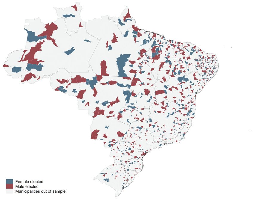
To assess whether our sample is representative of the evolution of COVID-19 in Brazil, we
plot the number of COVID-19 deaths over time separately for our sample of analysis and for
all Brazilian municipalities. As shown in Appendix Figure A2, the two samples experienced
a similar number of deaths per capita throughout the period of analysis. The same is true
when looking at the share of phone users staying at home over time (Appendix Figure
A3). Finally, Appendix Table A2 presents the share of municipalities that implemented
inhabitants and thus had single-round elections.
14a given containment policy at least once during the period of analysis, separately for our
sample and for a representative 10 percent random sample of municipalities obtained from
Chauvin et al. (2021). As for the random sample of municipalities (first two columns),
around 90 to 95 percent of municipalities in our sample implemented school closures,
gathering restrictions, events cancellation and made facemasks mandatory. In the analysis,
we will focus on the remaining six policies for which we have enough variation across
municipalities: commerce restrictions, curfew, lockdown, transport restrictions, travel
restrictions, and workplace restrictions.
Table 1: Descriptive statistics
Mean Sd Min Max Obs
Panel A Socio-demographic characteristics
population 13,932 12,714 1,037 91,311 983
experienced density 119.7 186.2 0.005 3468 983
average persons per room 0.704 0.243 0.435 4.282 983
commuting time 21.6 4.57 9.03 44.6 983
≥65 years old 0.083 0.023 0.022 0.179 983
nursing home residents per 10k pop 3.734 11.477 0.000 209.9 983
area 1,763 5,472 26.51 84,568 983
distance sao paulo 1,446 739.8 49.49 3,441 983
km to closest airport connecting to hot spots 300.9 214.6 23.07 1,557 983
median household income p/c 319.6 144.1 80.00 836.5 983
informality rate 0.169 0.055 0.036 0.418 983
unemployment rate 0.044 0.021 0.000 0.173 983
college graduate employment share 0.067 0.030 0.005 0.192 983
black and mixed population share 0.591 0.214 0.019 0.933 983
Panel B Political characteristics
turnout 0.855 0.059 0.673 0.980 983
number candidates 2.680 0.954 2.000 9.000 983
center-right & liberal 0.383 0.309 0.000 1.000 983
left 0.070 0.169 0.000 1.000 983
center-left 0.251 0.278 0.000 1.000 983
right & Christian 0.296 0.287 0.000 1.000 983
Notes: The sample includes only municipalities outside of any "arranjos populacionais", where one man and
one woman were the two front runners in the 2016 election. Socio-demographic variables come from the
2010 census, except for the experienced density that is defined as the total population living within 10 km
of the average inhabitant of the municipality and which is computed using the 2015 data from the Global
Human Settlement Layer. The political variables refer to the first round of the 2016 municipal election. The
last four variables denote the vote share of each of the four main political orientations.
153.2 Specification
We define the running variable X as the victory margin of the female candidate (the
difference between her vote share and the vote share of the male candidate), and the
treatment variable T as an indicator equal to 1 if the winner is a woman (X > 0) and 0 if
the winner is a man (X < 0). We assess the impact of having a female mayor using the
following specification:
Yi = αi + τ Ti + β1 Xi + β2 Xi Ti + µi (1)
where i indexes municipalities.
We use a nonparametric estimation method, which amounts to fitting two linear re-
gressions on each side of the threshold (Imbens and Lemieux, 2008; Calonico et al., 2014).
We follow Calonico et al. (2014)’s estimation procedure that provides robust confidence
intervals, and we use the data-driven MSERD bandwidths developed by Calonico et al.
(2019) that reduce potential bias the most. In Appendix F, we show the robustness of the
main results to using a second order polynomial and a wide range of different bandwidths.
As shown in Appendix Table G3, municipalities close to the threshold are very similar
to the average municipality in the full sample, in terms of both socio-demographic and
political characteristics.17
When presenting the RD results graphically, we follow Calonico et al. (2017): we focus
on observations in the estimation bandwidths and we use a linear fit and a triangular
kernel, so that the polynomial fit represents the RD point estimator.
3.3 Validity of the design
Density and balance tests
The identification assumption is that all municipalities’ characteristics change continuously
at the discontinuity, so that the only discrete shift is the change in the mayor’s gender. This
assumption can be violated if candidates are able to sort themselves across the threshold,
which would require them to be able to predict and manipulate their vote share with
extreme precision.
17
For the descriptive statistics, we define municipalities close to the threshold as municipalities where the
victory margin is smaller than 4 percentage points. Instead, the estimation bandwidths used in the analysis
vary with the outcomes, as they are data-driven.
16We perform several tests to bring support for this identification strategy. First, we test
for a jump in the density of the running variable using both McCrary (2008)’s method and
Cattaneo et al. (2018)’s procedure. As shown in Appendix Figures G1 and G2, the victory
margin of the female candidate is smooth at the discontinuity. The p-values associated
with the density tests are 0.26 and 0.19, respectively.
Second, we test for the balance of municipalities’ characteristics at the threshold using
a general balance test, following Anagol and Fujiwara (2016) and Pons and Tricaud (2018).
We regress the treatment variable on all 20 covariates presented in Table 1, predict the
treatment status of each municipality using the regression coefficients, and test for a jump
in the predicted value at the discontinuity. As shown in Figure 3 and Table 2, there is
no significant jump at the threshold and the point estimate is small and not significant.
In Figure 3 as in all the following RD graphs, each dot provides the average value of
the outcome within a given bin of the running variable. Observations on the right of
the discontinuity correspond to female-led municipalities, while observations on the left
correspond to male-led municipalities.
Figure 3: General balance test
1
.8
Predicted treatment
.6
.4
.2
0
-.1 -.05 0 .05 .1
Running variable
Notes: This figure is constructed by restricting the support to observations in the estimation bandwidths
and by setting the fit to match the local polynomial point estimator (polynomial order 1 and triangular
kernel). Dots represent the local averages of the treatment variable (indicator equal to one if the female
candidate won in 2016) predicted by a set of 20 municipal characteristics. Averages are calculated within
evenly-spaced bins of the running variable. The running variable is the margin of victory of the female
candidate in the 2016 election (percentage point difference between the vote share of the female and the male
candidates). Positive values denote that the female candidate won the election, and negative values that the
male candidate prevailed.
17Table 2: General balance test
(1)
Outcome Predicted Treatment
Treatment 0.020
(0.014)
Robust p-value 0.280
Observations 517
Polyn. order 1
Bandwidth 0.120
Mean, left of threshold 0.420
Notes: The outcome is the treatment variable predicted by a set of 20 municipal characteristics, as described
in the text. The independent variable is an indicator equal to one if the female candidate won in 2016. We
use a non-parametric estimation procedure (fitting two linear regressions separately on each side of the
threshold) and we use MSERD data-driven bandwidths. We assess statistical significance based on the robust
p-value. ***, **, and * indicate significance at 1, 5, and 10 percent, respectively. The mean gives the average
value of the outcome for male-led municipalities at the threshold.
We also test for a jump in each of the baseline characteristic taken individually (tables
and graphs in Appendix B). Only one variable out of 20 is significant at the 5 percent level.
Taken together, these results suggest that there is no sorting at the discontinuity. Further-
more, we show that the main results are robust in magnitude and statistical significance to
controlling for the whole set of covariates (Appendix F).
Gender vs. other characteristics of the winner
The use of a RDD ensures that the gender of the mayor is as good as randomly assigned
across municipalities at the threshold. However, it does not ensure that our results can be
interpreted as a gender effect if gender is correlated with other characteristics. For instance,
if female candidates are more likely to be from a left-wing party, our estimation might be
capturing the impact of political ideology instead of gender.
Looking at the characteristics of all 2016 candidates, we see that female candidates are
very similar to the average male candidate, in terms of age, incumbency status, and political
orientations (Appendix Table G4). One exception is education, as female candidates are
much more likely to have completed higher education compared to male candidates (72.4
vs. 49.3 percent, on average).
Ultimately, we are interested in whether female candidates barely winning against male
18candidates are similar to male candidates barely winning against female candidates. To
formally assess whether our effects could be driven by observable characteristics other
than gender, we take as outcomes the characteristics of the winner and test for a jump at
the threshold. As shown in Table 3 and Appendix Figure B2, while the winner appears
less likely to be the incumbent and more likely to have completed higher education when a
female candidate won, no coefficient is significant, or close to significance. We further show
that controlling for such characteristics leaves the results virtually unchanged (Appendix
F). We are thus confident that our results can be interpreted as a gender effect, rather than
coming from political experience (incumbency), age, education or ideology.
Table 3: Balance test: characteristics of the winner of the election
(1) (2) (3) (4) (5) (6) (7)
Outcome Incumbent Age Education Center-right Right Left Center-left
& Liberals & Christians
Treatment -0.040 -0.833 0.155 0.051 -0.039 -0.015 0.030
(0.076) (1.935) (0.099) (0.073) (0.076) (0.044) (0.080)
Robust p-value 0.586 0.818 0.297 0.427 0.479 0.840 0.651
Observations 606 570 483 677 659 516 579
Polyn. order 1 1 1 1 1 1 1
Bandwidth 0.141 0.131 0.107 0.163 0.155 0.119 0.133
Mean, left of threshold 0.260 48.972 0.445 0.311 0.333 0.071 0.270
Notes: In column 1 (resp., 3, 4, 5, 6, 7), the outcome is an indicator variable equal to 1 is the winner of the 2016
election is the incumbent (resp., has completed higher education, is from the political orientation center-right
and liberals, right and Christians, left, or center-left). In column 2, the outcome is the age of the 2016 winner
at the time of the first round. The independent variable is an indicator equal to one if the female candidate
won in 2016. We use a non-parametric estimation procedure (fitting two linear regressions separately on
each side of the threshold) and we use MSERD data-driven bandwidths. We assess statistical significance
based on the robust p-value. ***, **, and * indicate significance at 1, 5, and 10 percent, respectively. The mean
gives the average value of the outcome for male-led municipalities at the threshold.
4 Results
4.1 Impact of having a female mayor on COVID-19 deaths
We start by looking at the impact of having a female mayor on the timing of the first reported
COVID-19 death. Table 4 and Figure 4 take as outcome the number of days between the last
day of 2019 – when the first known case of COVID-19 was reported worldwide – and the
first death attributed to the disease in the municipality. We obtain a coefficient close to zero
and non-significant, showing that the first death occurred at the same time on average in
female- and male-led municipalities (around July 23, 2020, 205 days after the first reported
19case worldwide).
Table 4: Impact on the timing of the first reported COVID-19 death
(1)
Outcome Date of the first death
Treatment -1.101
(13.151)
Robust p-value 0.960
Observations 595
Polyn. order 1
Bandwidth 0.142
Mean, left of threshold 204.708
Notes: The outcome is the the number of days between 12/31/2020 and the first death. It is missing for
20 municipalities in which no death occurred up to May 9, 2021 (day at which the data were generated).
The independent variable is an indicator equal to one if the female candidate won in 2016. We use a non-
parametric estimation procedure (fitting two linear regressions separately on each side of the threshold) and
we use MSERD data-driven bandwidths. We assess statistical significance based on the robust p-value. ***,
**, and * indicate significance at 1, 5, and 10 percent, respectively. The mean gives the average value of the
outcome for male-led municipalities at the threshold.
Figure 4: Impact on the timing of the first reported COVID-19 death
300
# days between 12/31/2019 and 1st death
250
200
150
-.2 -.1 0 .1 .2
Running variable
Notes: This figure is constructed by restricting the support to observations in the estimation bandwidths and
by setting the fit to match the local polynomial point estimator (polynomial order 1 and triangular kernel).
Dots represent the local averages of the number of days between 12/31/2020 and the first death. Averages are
calculated within evenly-spaced bins of the running variable. The running variable is the margin of victory
of the female candidate in the 2016 election (percentage point difference between the vote share of the female
and the male candidates). Positive values denote that the female candidate won the election, and negative
values that the male candidate prevailed.
20Given that having a female mayor did not affect the timing at which municipalities
started to experience fatalities from the virus, we can use the same time frame to study
the evolution of COVID-19 deaths in female- and male-led municipalities. We look at the
impact on the total number of deaths in the four main periods characterizing the evolution
of COVID-19 in Brazil (see Figure 1): beginning of the first wave (April-May 2020), peak
of the first wave (June-August 2020), end of the first wave (September-October 2020), and
beginning of the second wave (November 2020-January 2021). We normalize the number
of deaths by the 2010 population and multiply by 10,000 so that the outcome measures the
total number of deaths in the municipality per 10,000 inhabitants.18
As shown in Table 5, on average, having a female mayors led to a 0.39 increase in the
number of deaths per 10,000 inhabitants in the first period, a coefficient significant at the
5 percent level. This represents more than a twofold increase compared to the average
number of deaths in male-led municipalities at the threshold. Conversely, we find that
female-led municipalities experienced 1.0 fewer deaths per 10,000 inhabitants in the last
period, on average. This effect is significant at the 5 percent level and corresponds to a 41.1
percent decrease compared to male-led municipalities. We find no effect during the second
and third periods, corresponding to the middle and end of the first wave. The coefficients
are not significant and the point estimates are much smaller, both in absolute terms and
compared to the means.
Figure 5 plots the number of deaths against the running variable for each period sepa-
rately. Consistent with the formal estimation, we see an upward jump at the threshold at
the beginning of the first wave, a downward jump at the end of the period of analysis, and
no significant jumps for the other two periods.
Appendix Table C2 and Appendix Figure C2 further assess the impact month by month.
We find that the positive impact in the first period is driven by a larger number of deaths in
female-led municipalities in May 2020, while the negative impact in the last period is driven
by a lower number of deaths in female-led municipalities in November and December
2020.
Finally, we look at how these effects translate into the evolution of the number of
cumulative deaths. Figure 6 shows the estimated impact of having a female mayor on the
total number of deaths up to a given date, for each day from April 1 to January 31. Each
dot on the blue line provides the estimate for a given day, and the blue shaded area depicts
18
We start in April as no death occurred in municipalities part of our sample in March (a total of 201
occurred across the country).
21the 95 percent robust confidence intervals. Consistent with female-led municipalities
experiencing more deaths in May, the point estimates on the cumulative number of deaths
is positive and significant from mid-May to mid-June. It remains positive but not significant
up to October, when it becomes close to zero. Next, in line with female-led municipalities
experiencing fewer deaths in November and December, the point estimates become negative
starting in mid-November, after the first round of the 2020 election.
Overall, we find that having a female mayor reduced the cumulative number of deaths by
0.97 as of January 31st 2021 (14.4 percent), on average, but the coefficient is not statistically
significant (Appendix Table C1 and Appendix Figure C1).
We next turn to the analysis of containment policies and mobility to explore what can
explain these patterns.
Table 5: Impact on COVID-19 deaths by periods
(1) (2) (3) (4)
Ouctome # COVID-19 deaths per 10,000 inhabitants
Period 1 Period 2 Period 3 Period 4
Treatment 0.387** -0.056 -0.198 -1.001**
(0.175) (0.510) (0.283) (0.405)
Robust p-value 0.037 0.846 0.472 0.016
Observations 580 498 673 514
Polyn. order 1 1 1 1
Bandwidth 0.134 0.113 0.160 0.118
Mean, left of threshold 0.206 2.580 1.384 2.434
Notes: Each column takes as outcome the total number of deaths per 10,000 inhabitants (using the 2010
census) during the period of interest. Period 1 (resp., 2, 3, and 4) corresponds to April-May 2020 (resp.,
June-August 2020, September-October 2020, and November 2020-January 2021). The independent variable is
an indicator equal to one if the female candidate won in 2016. We use a non-parametric estimation procedure
(fitting two linear regressions separately on each side of the threshold) and we use MSERD data-driven
bandwidths. We assess statistical significance based on the robust p-value. ***, **, and * indicate significance at
1, 5, and 10 percent, respectively. The mean gives the average value of the outcome for male-led municipalities
at the threshold.
22Figure 5: Impact on COVID-19 deaths by period
Period 1 Period 2
5 5
4 4
# deaths in Period 1
# deaths in Period 2
3 3
2 2
1 1
0 0
-.2 -.1 0 .1 .2 -.1 -.05 0 .05 .1
Running variable Running variable
Period 3 Period 4
5 5
4 4
# deaths in Period 3
# deaths in Period 4
3 3
2 2
1 1
0 0
-.2 -.1 0 .1 .2 -.1 -.05 0 .05 .1
Running variable Running variable
Notes: Each graph is constructed by restricting the support to observations in the estimation bandwidths
and by setting the fit to match the local polynomial point estimator (polynomial order 1 and triangular
kernel). Dots represent the local averages of the total number COVID-19 deaths per 10,000 inhabitants in
the municipality during the period of interest. Averages are calculated within evenly-spaced bins of the
running variable. The running variable is the margin of victory of the female candidate in the 2016 election
(percentage point difference between the vote share of the female and the male candidates). Positive values
denote that the female candidate won the election, and negative values that the male candidate prevailed.
Figure 6: Impact on the cumulative number of COVID-19 deaths day by day
Notes: This figure plots the RD estimates obtained by taking as outcome the cumulative number of Covid-19
deaths per 10,000 inhabitants, for each day from April 1st to January 31st, 2020.
234.2 Impact of having a female mayor on containment policies
We now explore whether female mayors pursued different policies than male mayors in
response to the COVID-19 crisis. As discussed in Section 2.3, we consider six policies:
workplace, commerce, travel, and public transport restrictions; lockdown; and curfews.
Appendix Figure G3 shows the frequency with which municipalities in our sample imple-
mented these policies between March 1 and October 31, 2020 — the period for which policy
data are available. Most municipalities only pursued the first four policies in the early
weeks of the pandemic. Curfews were only implemented in 13 and 25 municipalities in
March and April respectively; and no municipality in our sample implemented a lockdown
before May.
We first look at the impact of having a female mayor on the adoption of a given policy
by calendar month. For each policy and month, we define our dependent variable as the
total number of days in which the policy was in place in the municipality.
Table 6 presents the results for commerce restrictions. We find that female-led munici-
palities were significantly less likely to close commerce at the beginning of the pandemic.
On average, this policy was implemented 2.5 fewer days during the month of March in
female-led municipalities, a large effect relative to the average of 3.2 days in male-led
municipalities at the threshold. In April, the effect was of 6.5 fewer days relative to a
10.6 average. Both coefficients are significant at the 5 percent level. We further show that
these effects are driven by female mayors’ higher likelihood to delay the introduction of
commerce restrictions. We estimate the female-mayor effect on the number of days between
December 31, 2019 and the first day of implementation of each policy (Appendix Table
D1). On average, female-led municipalities implemented commerce restrictions 33 days
later than the average male-led municipality at the threshold, an effect that is significant at
the 5 percent level.
In contrast, we find that female-led municipalities became significantly more likely
to close commerce in the two months leading up to the November election. On average,
having a female mayor led to 7.3 and 7.5 more days of commerce closures in September
and October, respectively. These effects represent a two-fold increase relative to the average
in municipalities that barely elected a male, and they are both significant at the 10 percent
level. Figure 7 shows this pattern visually. While we see a large downward jump in March
and April, the discontinuity gradually disappears in subsequent periods, before turning
into large upward jumps in the last two months.
24You can also read