Journal of Urban Economics - Gwern.net

Journal of Urban Economics 122 (2021) 103318

 Contents lists available at ScienceDirect

 Journal of Urban Economics
 journal homepage: www.elsevier.com/locate/jue

The congestion costs of Uber and Lyft
Matthew Tarduno a,b,1,∗
a
 Department of Agricultural and Resource Economics, University of California, Berkeley, United States
b
 Energy Institute at Haas, United States

a b s t r a c t

I study the impact of transportation network companies (TNC) on traffic delays using a natural experiment created by the abrupt departure of Uber and Lyft from
Austin, Texas. Applying difference in differences and regression discontinuity specifications to high-frequency traffic data, I estimate that Uber and Lyft together
decreased daytime traffic speeds in Austin by roughly 2.3%. Using Austin-specific measures of the value of travel time, I translate these slowdowns to estimates
of citywide congestion costs that range from $33 to $52 million annually. Back of the envelope calculations imply that these costs are similar in magnitude to the
consumer surplus provided by TNCs in Austin. Together these results suggest that while TNCs may impose modest travel time externalities, restricting or taxing TNC
activity is unlikely to generate large net welfare gains through reduced congestion.

1. Introduction congestion. First, Uber and Lyft likely select entry locations based on
 trends in city-level characteristics unobservable to the econometrician.
 Transportation network companies (TNC) like Uber and Lyft have Comparisons that leverage differences in TNC entry dates across loca-
grown rapidly over the past decade to become integral parts of urban tions may therefore suffer from reverse causality. Second, within-city
transportation systems. A small but growing literature has attributed to time series regressions may be biased by omitted variables (e.g., gentri-
these companies benefits that include billions in annual consumer sur- fication) which are serially correlated with TNC activity and also impact
plus (Cohen et al., 2016), reductions in drunk driving (Greenwood and congestion.
Wattal, 2015), and flexible work (Judd and Krueger, 2016; Angrist et al., In this paper I leverage a natural experiment in Austin, TX to cir-
2017). cumvent these identification challenges: On May 9th , 2016, both Uber
 The costs of TNC expansion, however, have yet to receive commen- and Lyft unexpectedly exited Austin following a vote that upheld a city
surate treatment in the economics literature. Most notably, TNCs have ordinance requiring driver background checks. I combine this variation
been accused of contributing to traffic congestion (San Francisco Tran- in TNC activity with novel and granular Bluetooth traffic speed data,
sit Authority, 2018; Schaller Consulting, 2018), but existing studies of and setting-specific estimates of the value of travel time to answer two
the impact of TNCs on congestion are few, arrive at varied conclusions, research questions. First, do transportation network companies impact
and do not quantify the implied congestion costs (Li et al., 2019; Erhardt traffic congestion? And if so, what are the travel-time related costs or
et al., 2019). Back of the envelope calculations suggest these costs could benefits of TNC operation?
be substantial. A 2017 Inrix report, for example, placed the annual cost This setting informs two empirical strategies: a difference in differ-
of congestion to US drivers at $305 billion (Inrix, 2017)—roughly two ences comparing pre- versus post-May 9th traffic speeds in 2015 (where
orders of magnitude larger than estimates of national consumer surplus both companies operated year round) to 2016 (where both companies
provided by Uber (Cohen et al., 2016). This suggests that if TNCs have exit on May 9th ), and a regression discontinuity in time. Across specifi-
even a modest impact on traffic congestion, the negative externalities cations, I find evidence of modest increases in traffic speeds following
associated with lengthening travel times could offset consumer surplus the exit of Uber and Lyft. Difference in differences results suggest that
benefits. Understanding how and whether TNCs impact traffic conges- across all hours, traffic speeds increased roughly 1% following the exit
tion therefore plays a crucial role in determining appropriate policy re- of Uber and Lyft. 7 am. to 7 p.m. traffic speeds increased by 2.3%, with
sponse to the continued growth of these companies. the largest TNC-related slowdowns occurring during the middle of the
 Two identification problems, however, make causal inference diffi- day (11 a.m. to 2 p.m.). Using setting-specific estimates of value of the
cult when studying the relationship between TNC activity and traffic travel time, I calculate that Austinites would be willing to pay roughly

 Correspondence to: Department of Agricultural and Resource Economics, University of California, Berkeley, United States.
 ∗

 E-mail address: tarduno@berkeley.edu
 1
 I thank Michael Anderson, James Sallee, Meredith Fowlie, Aprajit Mahajan, Matthew Gibson, Alejandro Favela Nava, Jenya Kahn-Lang, the participants of the
2019 Giannini Foundation of Agricultural and Resource Economics Student Conference, as well as the Editor (Matthew Turner) and this paper’s two anonymous
reviewers for their valuable feedback. I also thank John Clary at the Austin Transportation Department for providing technical support during the data acquisition
phase.

https://doi.org/10.1016/j.jue.2020.103318
Received 22 October 2019; Received in revised form 25 November 2020
Available online 21 January 2021
0094-1190/© 2020 Elsevier Inc. All rights reserved.

M. Tarduno Journal of Urban Economics 122 (2021) 103318

$33 to $52 million annually to avoid these slowdowns. Back of the enve- spend a significantly higher fraction of their time with a passenger in
lope calculations suggest that these figures are a small fraction (4–6%) of their vehicle than do taxi drivers. This ride-sharing effect could atten-
total Austin-area congestion costs, and are roughly the size of estimates uate or outweigh the effect of induced trips. There may also be com-
of the consumer surplus associated with TNC operation in Austin. plementarities between TNCs and public transit: Hall et al. (2018) use
 These findings improve on the existing literature in three ways. First, a difference in differences design on measures from the National Tran-
this is to my knowledge the only paper to use the exit of Uber and Lyft sit Database to conclude that Uber is indeed a complement to public
to study the impacts of TNCs on congestion. This translates to weaker transportation. It is unclear, though, whether complementarity between
identifying assumptions than those imposed in analyses leveraging the TNCs and public transit will result in more or fewer vehicle trips.
staggered expansion of these companies. Second, I extend existing anal- To date there exists little econometric work on whether TNCs cause
yses by mapping changes in travel speeds to changes in travel time costs, traffic congestion, and existing results arrive at varied conclusions.
providing the first estimates of the congestion costs associated with TNC Li et al. (2019), for example, use city-level congestion measures and
activity. And third, the spatial and temporal granularity in the Bluetooth differences in Uber’s entry date to estimate the company’s impact on
data allows me to perform analyses that contribute to a more complete congestion, concluding that Uber improves city-level congestion mea-
picture of the heterogeneous impacts of TNC activity on traffic conges- sures. Erhardt et al. (2019), on the other hand, use 2010 and 2016 Inrix
tion. traffic data and scraped measures of Uber activity to calibrate a traf-
 These findings also provide several important takeaways for policy- fic engineering model of San Francisco. They conclude that rideshar-
makers. First, TNC activity can be viewed roughly as a transfer, as the ing companies were responsible for significant (30%) increases in ve-
consumer surplus enjoyed by TNC passengers is of similar size to the hicle hours traveled. In addition to the fact that these studies reach
time loss incident on incumbent drivers. Second, it is difficult to ratio- contradicting conclusions, the identification concerns outlined in the
nalize TNC quantity restrictions purely on welfare grounds, as the lost introduction suggest value in reassessing this question using a natural
consumer surplus may outweigh travel time gains. In other words, even experiment.
if TNC regulation is more politically achievable than are price-based
congestion controls, TNC regulation appears (at least in the Austin case) 3. Natural experiment
to be a poor tool to address congestion-related externalities. Relatedly,
the relatively modest impacts of TNCs on traffic congestion in Austin Austin, TX, is the 11th largest incorporated place in the United States
suggest that congestion taxes targeted specifically at ridesharing com- and suffers from considerable congestion: According to Inrix, Austin
panies are unlikely to result in large traffic-related welfare gains. Lastly, ranked 14th nationally and 72nd globally in the number of average hours
the fact that speeds slow in response to TNC activity suggests TNCs add lost to congestion per driver. Cities with similar levels of per-driver con-
vehicles miles traveled (VMT) to the transit system. In other words, the gestion costs include San Diego, Berlin, and Manchester. Both Uber and
VMT avoided by sharing rides are outweighed by additional trips in- Lyft began operating in Austin in 2014.
duced by the availability of TNCs. In December 2015, the Austin City Council passed Ordinance No.
 The rest of this paper is organized as follows. Section 2 describes 20151217-075, which imposed a series of regulations on TNCs, includ-
related literature and background. Section 3 details the events that pre- ing data requirements, restrictions on idling locations, and most con-
cipitated the departure of Uber and Lyft from Austin. Section 4 outlines troversially, fingerprinting requirements to facilitate driver background
the data sources. I describe my empirical strategy and threats to identifi- checks (The City Council of Austin, 2015). Proposition 1, sponsored by
cation in Section 5, and present results in Section 6. Section 7 concludes. Uber and Lyft, attempted to overturn this ordinance. On May 7th , 2016,
 the Proposition was defeated in a citywide vote, with 56% of voters
2. Background and related literature casting against (The Texas Tribune, 2016). In protest, Uber and Lyft ex-
 ited the Austin market on May 9th (New York Times, 2016). 13 months
 Traffic congestion is a significant urban disamenity. It is costly later, Uber and Lyft re-entered Austin as Governor Greg Abbott signed
(Inrix, 2018), it is associated with lower self-reported happiness into law HB 100, which overturned Austin’s local ordinance (The 85th
(Anderson et al., 2016), and it comes with considerable co-costs in terms Texas Legislature, 2017). This variation in TNC activity provides the
of noise and pollution (Currie and Walker, 2011). Although a tax is the basis for my empirical identification.
canonical policy prescription for congestion (Vickrey, 1969), both the- During the yearlong absence of Uber and Lyft, Austin was not with-
ory and empirics suggest that because targeting individual contributions out ridesharing. A number of smaller TNCs entered the market or ex-
to congestion is difficult, realistic congestion pricing instruments (e.g., panded their Austin presence following the defeat of Proposition 1. In
cordon charges) may fall well short of the welfare gains achievable by date of their arrival in Austin, these companies are: GetMe (Decem-
a hypothetical first best policy (Knittel and Sandler, 2018; Prud’Homme ber 2015), Fare (Mid-May 2016), Fasten (June 1st , 2016), Tride Tech-
and Bocarejo, 2005). This, coupled with the potential political advan- nologies (June 15th , 2015), and RideAustin (June 16th , 2016). Wingz,
tage of TNC regulation over comprehensive congestion taxation suggests which provides rides to and from the airport, also started operating in
that understanding the sign and magnitude of TNC related time costs or Austin in May of 2016. A survey of Austin commuters conducted in
savings will be important for informing city-level policy. Indeed, sev- November 2016 by Hampshire et al. (2017) offers a view of take up of
eral cities have already moved to regulate TNCs in the name of con- these alternative rideshare companies. RideAustin held the largest mar-
gestion. New York City, for example, cited congestion as a motivation ket share (47.4%), followed by Fasten (34.5%), Fare (12.9%), GetMe
for its 2018 ridesharing cap (New York Times, 2018). As of 2020, San (2.8%), Wingz (1.6%), and Tride (0.4%). Informed by the Hampshire
Francisco, New York, and Chicago have all imposed “congestion fees,” et al. (2018) survey and the universe of RideAustin’s 2016 trip-level
levied on TNC trips in the city center (New York Times, 2019). Outside data, I am able to infer the level of total TNC activity in Austin follow-
of the US, cities like London and Vancouver have weighed congestion ing the exit of Uber and Lyft. I can therefore identify a window following
impacts as they deliberate over TNC policy (Reuters, 2019; Vancouver the Proposition 1 vote where alternative TNC activity is negligible (see
Sun, 2019). Section 5.1).
 As a number of other observers have noted, however, the impact
of TNCs on traffic speeds is theoretically ambiguous. While survey 4. Data
data from Rayle et al. (2014) and Clewlow and Mishra (2017) suggest
TNCs induce trips, and Mangrum and Molnar (2018) demonstrate that I use data collected from an array of Bluetooth sensors along major
taxis—the closest analog to TNCs—increase congestion on the margin, roadways (both highway and surface-level) operated by the Austin
Judd and Krueger (2016) show that in five of six US cities, Uber drivers Department of Transportation. Located inside traffic signal cabinets,

 2

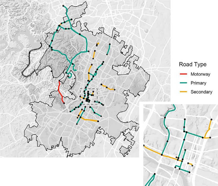
M. Tarduno Journal of Urban Economics 122 (2021) 103318

 Fig. 1. Bluetooth Segment Locations in Austin,
 TX. Notes: Nodes represent terminal Bluetooth sen-
 sor locations for each of the 79 segments used in
 my analysis. Note that some sensors act as both
 origin and destination readers for different seg-
 ments. Paths represent Google Maps recommended
 driving directions between endpoints of a given
 segment, colored by Open Street Map road type.
 Motorways are major divided highways, primary
 roads are large multi-lane roads that may or may
 not be divided. Secondary roads are typically two-
 to four-lane surface streets. The black line is the
 Austin city limit.

these sensors detect unpaired Bluetooth devices (e.g., smartphones, car responds to 20.06 miles per hour. This figure is consistent with periods
systems) and estimate traffic speeds based on the movement of single of significant congestion.
devices (which are given unique anonymous identifiers) through the My variable of interest is minutes per mile, which has two advan-
network of sensors. tages over miles per hour. First, a change of one mile per hour does not
 I use an aggregated version of this dataset prepared by Post Oak represent a constant damage over the domain of this variable: In terms
Traffic Systems, which isolates device movements through specific road of time lost, changing from 5 to 4 miles per hour is roughly 20 times
segments (henceforth segments), which are short sections along just as costly as changing from 20 to 19 miles per hour. Second, multiply-
one road. This company pre-processes the data in several ways. Data ing outcomes in minutes per mile by estimates of the value of time is a
are aggregated at 15 min bins and represent the average speed across straightforward way to arrive at cost calculations from changes in traffic
the segment for devices that appear at the origin reader first, and then delays.
the destination reader, and do not appear at any other sensors in the While novel and granular, the Bluetooth data bring challenges for
interim. These data are also filtered for outliers: only observations that estimation. First, in the raw data available on the Austin Open Data
fall within 75% of the IQR of the previous 15 observations are used in Portal, 61 of the 79 segments used in my analysis show the segment
calculating speeds. This type of filtering is applied to combat bias from length changing over the course of the study period. While most of these
the movement of non-vehicle Bluetooth devices (like those carried by adjustments are minor, and personal correspondence with Austin Trans-
pedestrians) through the sensor network. portation Department employees suggests that these adjustments likely
 In addition to the data cleaning performed by Post Oak Traffic Sys- reflect updated length measurements and not relocation of Bluetooth
tems, I further restrict my sample to consistently reporting sensors. Of sensors, I nonetheless investigate the possibility that these segment
the 430 total segments, I drop segments that report in fewer than 70% length changes constitute a threat to identification in Appendix E. I
of days during each year (2015 and 2016) of the study period, leav- use the updated length measurements for all speed calculations in all
ing me with a panel of 79 segments. For robustness I also report re- time periods. A second challenge is the possibility of Bluetooth sensors
sults using a) all segments that report in more than 30% of study pe- measuring the movement of pedestrians. If filtering does not eliminate
riod days and b) only segments that report during 100% of study period all measurement error originating from Bluetooth devices used by
days. Austinites walking or biking, and the use of these modes of transit
 The 79 segments I use in my preferred specification are plotted in is correlated with the period where Uber and Lyft exited Austin, the
Fig. 1 and summarized in Table 1. The mean segment length is 0.72 empirical strategies I describe below will arrive at biased estimates. I
miles, with minimum and maximum lengths of 0.06 and 3.8 miles, re- further investigate this in Section 5.4.
spectively. As shown in Fig. 1, my sample covers a range of road types. I compile several other datasets to augment my analysis. To control
The smallest roads in my sample are two-lane roads, the largest are 7- for weather-related shocks, I use precipitation and temperature data ac-
lane roads, and the median segment is a 5-lane road. I observe 966,301 cessed through the National Oceanographic and Atmospheric Admin-
15-min speed reports during my study period. On average, a segment istration’s National Centers for Environmental Information. To isolate
sees 4.77 devices move from origin to destination during each 15 min a period of time where the impact of other TNCs is minimal, I use
period, meaning that my data summarize roughly 4.6 million segment RideAustin’s trip-level data. These data range from June 2nd , 2016 to
traverses. The average travel speed is 2.99 minutes per mile, which cor- April 13th , 2017, and are publicly available online (RideAustin, 2017).

 3

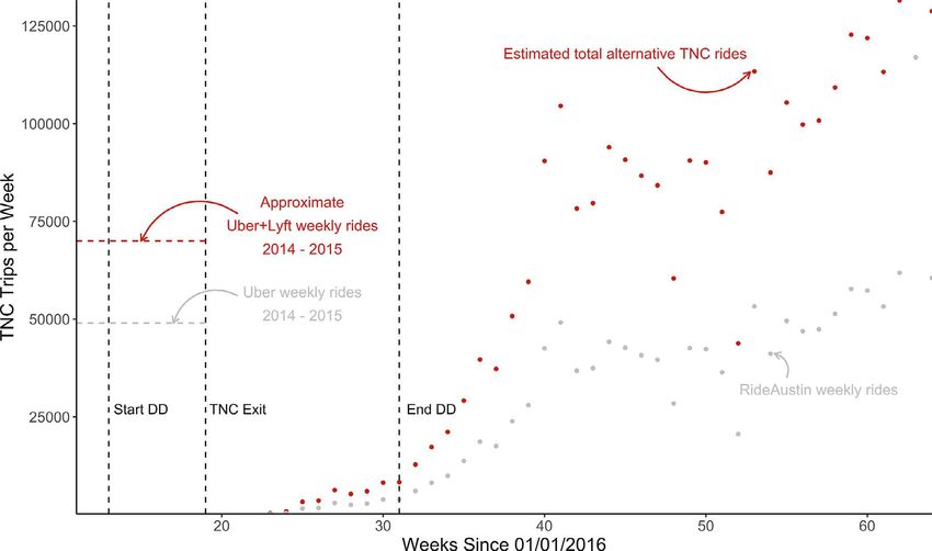
M. Tarduno Journal of Urban Economics 122 (2021) 103318

Fig. 2. Variation in TNC Activity. Notes: This figure displays the variation in ridesharing activity I use to identify the impact of TNCs on congestion. From left to
right, the vertical lines represent the start of the 2016 difference in differences period (March 20th ), the failure of Proposition 1 (May 9th ), and the end of the 2016
difference in difference period (August 1st ). The grey dotted line is the average number of Uber trips per week (as per an Uber Report on 2014–2015 operations).
The red dotted line represents an estimate of total Uber and Lyft pre-exit activity, assuming a 30% Lyft market share. Note that because both Uber and Lyft entered
Austin in 2014, the actual number of Uber trips in early May 2015 was likely much larger than 70,000 per week. The grey dots plot weekly RideAustin activity for
the first 9 months of the company’s operation. The red dots inflate the RideAustin data by the reciprocal of its November 2016 market share (47%) to provide an
estimate for the total level of post Proposition 1 alternative TNC activity.

Lastly, I use two datasets to arrive at setting-specific value of time esti- ences specifications using later years, I am able to use data from dif-
mates. The first is the National Household Travel Survey (NHTS), which ferent parts of 2017–2019 to perform placebo regression discontinuity
contains information on income and commuting habits. The second is estimates (see Appendix D).
a toll price and travel time dataset from the MoPac variable price free-
way in Austin. These data were provided courtesy of the Central Texas 5.2. Difference in differences
Regional Mobility Authority and are further detailed in Appendix A.
 To study the effect of the exit of Uber and Lyft on travel times, I com-
5. Empirical strategy pare traffic speeds pre and post May 9th in 2016 (where Uber and Lyft ex-
 ited) to 2015 (where both companies operated year-round). To capture
5.1. Timeframe heterogeneity in the congestion impacts across time of day, I perform
 this comparison within each hour of day, ℎ (or equivalently, interacting
 I use Bluetooth traffic data from 2015 and 2016 to study the rela- each right-hand side term below with an hour of day dummy):
tionship between TNCs and congestion. I truncate this window to isolate
periods where the variation in traffic speeds can be credibly attributed , , = + ℎ + 1 + 2 + 3 ⋅ + 4 + , + , , (1)
to the failure of Proposition 1. As described in Section 3, a number of
TNCs entered the market following the exit of Uber and Lyft. Estima- Where , , is the speed (in minutes per mile) measured over segment 
tions using the entire yearlong suspension period as a comparison would on day of year . is a dummy that equals one for the year 2016, and
therefore underestimate any changes relative to a TNC-free counterfac- is a dummy that equals one for days (in any year) after May 9th . 
tual. Informed by the universe of trips from RideAustin—the TNC with is a set of dummies for each road segment, and is the signed number
the largest market share during Uber and Lyft’s absence—I truncate my of days between a given date and May 9th of that year. is a vector of
estimation period on August 1st , 2016. Similarly, Austin hosts the South controls that includes day of week fixed effects, holiday fixed effects, 10
by Southwest Music Festival (SXSW) each March. I restrict my analysis 10-degree daily temperature bins, and 10 daily precipitation level bins.
to exclude the 2015 and 2016 festivals. This leaves me with data from The interacton betwen is the treatment indicator, as it takes a value
March 20th to August 1st for both 2015 and 2016. The 2016 study pe- of 1 for observations after May 9th , 2016, and zero otherwise. ⋅ are
riod is plotted with TNC data in Fig. 2. Note that although the Austin segment-year specific linear time trends.
Bluetooth data extend through 2019, significant portions of the spring The identifying assumption in the estimation of ℎ —the effect of
are missing data from years 2017, 2018, and 2019, including Uber and Uber and Lyft operation on travel speeds during a given hour of day
Lyft’s re-entry in May of 2017. While this rules out difference in differ- ℎ—is that conditional on seasonality and weather, the difference in

 4

M. Tarduno Journal of Urban Economics 122 (2021) 103318

travel speeds between 2016 and 2015 at hour ℎ does not change after timates, traffic speed must be mismeasured, and that mismeasurement
May 9th for reasons other than the operation of Uber and Lyft. must be correlated with the treatment.
 I calculate hour-specific congestion impacts with the goal of produc- Data on mode shares and mode speeds suggest that this type of bias
ing more accurate cost estimates. As I show in Appendix A, variable-toll cannot alone account for my results. Hampshire et al. (2017) suggest
data suggest that the value of travel time in Austin varies significantly 1.8% of TNC users switched to bikes following Uber’s exit. If TNCs made
from hour to hour. Similarly, the number of vehicles on the road peaks up 10% of Austin trips, and bikes constituted 1.53% (United States Cen-
during rush hours. Together, this information suggests that the same sus Bureau, 2015), this mode shifting represents an 11.8% increase in
change in traffic speeds could produce different aggregate congestion total bike trip volume. The average car in my sample took 2.99 min
costs at different times of day. By matching hour-specific estimates of to traverse a mile—3.01 minutes per mile fewer than the 6 minutes
the impact of TNCs to hour-specific vehicle miles traveled (VMT) and per milemph) assumed by Google biking directions. These figures im-
hour-specific estimates of the value of travel time, my cost calculations ply that for changes in bike shares to alone account for a change of
account for temporal heterogeneity that pooled estimates may not re- 0.1 minutes per mileroughly the average treatment effect across day-
flect. To determine whether the convolution between hourly congestion time hours), bikes would need to constitute roughly 28% of observed
impacts and hourly VOT is a first-order consideration, I also estimate Bluetooth samples after dropping extreme travel time outliers. This fig-
a model pooling across hours of day. This estimator is Eq. 1, but run ure is inconsistent with the travel speeds implied by the movement of
without interacting hour of day fixed effects with the right hand side Bluetooth devices, which greatly exceed 10 miles per hour on average.
variables. The rationale for this regression is to simulate what estima- Nonetheless, I draw on a second traffic speed dataset to empirically
tion and inference might look like using temporally aggregated data. examine this concern. In addition to Bluetooth sensors, the city of Austin
 To investigate spatial heterogeneity, I estimate a model pooling over also maintains pneumatic sensors that take periodic measurements of
hours of day and allowing an idosyncratic treatment effect for each road traffic speeds. While these measurements are not frequent enough to
segment. This model is equivalent to Eq. 1, but interacts the set of seg- act as a replacement dependent variable, they do allow me to study
ment dummies with the treatment indicator, . is now a 1x79 vector the relationship between Bluetooth speed measurements and true traffic
of segment-specific treatment effect estimates. Note that in this pooled speeds by matching segments to pneumatic sensors.
Equation hour of day fixed effects are included in , . While we should not expect pneumatic sensors to match segment
 speeds exactly (segments often include intersections), if there is signifi-
 , , = + + 1 + 2 + 3 ⋅ + 4 + , + , , (2) cant switching to non-vehicular modes of transport that biases the Blue-
 tooth speed measurements, this would be reflected in a change in the
5.3. Regression discontinuity relationship between the two measurements. For example, say we have
 a segment-sensor pair, and prior to May 9th , 2016, when the pneumatic
 Lastly, I estimate a regression discontinuity model, again estimat- sensor reports a speed of 25 mph, the Bluetooth segment on average re-
ing hour-specific treatment effects ( ℎ ) by interacting each term in the ports a speed of 20 mph. If there is bias from mode-switching, we would
regression Equation with a set of hour of day fixed effects. expect this relationship to change in the post period. Now, when the
 , = + ℎ + 1 + 2 ⋅ + 2 1 ⋅ 2 + 4 + + , (3) pneumatic sensor again registers 25 mph, the incresed number of non-
 filtered pedestrian datapoints biases the segment measurement down-
The identifying assumption for ℎ is that conditional on weather, po- ward, to, say, 18 mph.
tential outcomes (traffic speeds) in hour of day ℎ are continuous about To operationalize this anecdote, I match segments to pneumatic sen-
May 9th , 2016. While the identifying assumption for the RD is arguably sors, and run a regression of segment speeds on sensor speeds, allowing
weaker than that of the difference in differences estimator, the RD will for a differential slope term interacted with a post May 9th 2016 dummy.
produce estimates of the short-term response to the exit of Uber and If I find a statistically (and economically) significant difference in slopes,
Lyft. As such, I rely on the difference in difference estimator to produce I treat this as evidence of mode choice related bias. This exercise is de-
my preferred annual congestion cost figures. tailed in Appendix B. I match 39 Bluetooth segments to pneumatic road
 sensors. In a simple regression with month of year and road segment
5.4. Threats to identification fixed effects, I find little evidence to support pedestrian-induced bias
 in my estimates. As shown in Table B.1, the coefficient on the interac-
 Threat 1: Contemporaneous shocks. The identifying assumptions tion between the post dummy and the pneumatic segment speed is not
in both the RD and DID estimates rely on the absence of ∗ - statistically different from zero, nor is it of meaningful magnitude.
specific shocks to Austin area travel speeds. The end of the University of Threat 3: TNC driving speeds. If TNC vehicles drive significantly
Texas, Austin (UT) school year, for example, presents a potential threat slower or faster than the average non-TNC vehicle in a way that re-
to identification if university-related traffic activity differed substan- mains after filtering, the above estimates of ℎ will be biased. During
tially between 2015 and 2016. In Appendix D, I use placebo exit dates congested conditions it is unlikely that this should occur: if congestion
to determine whether or not shocks that create regression discontinuity slows all drivers, then travel time measurements from any subset of ve-
estimates on the order of my reported coefficients are empirically com- hicles should be representative of average speeds. At free-flow traffic
mon. Fig. D.2 displays coefficient estimates using the actual exit date in speeds, however, it is possible that TNCs drive faster (due to profit mo-
relation to the distribution of coefficients from 134 regression disconti- tive) or slower (idling to find riders) than non-TNC vehicles.
nuities using placebo exit dates, 13 of which were chosen to line up with To test these concerns, I use public trip-level data from the startup
the beginning/end of a UT semester. 5 of the 134 placebo coefficients RideAustin, which entered the market following the departure of Uber
(4%) are more negative than the estimates using the actual TNC exit and Lyft. Following Mangrum and Molnar (2018), who construct “taxi
date, zero of which correspond to the start/end of a UT semester. This races” to test whether different types of taxi travel at different speeds,
placebo test therefore suggests that shocks that produce RD estimates on I match RideAustin trips to Bluetooth segments, allowing me to test the
the order of my estimates are empirically uncommon, and that my re- null hypothesis that TNC vehicles drive at the same speeds as the average
sults are not likely a result of changing traffic patterns related to activity mix of vehicles.
at UT. This exercise is detailed in Appendix C. Over 221 trip-segment
 Threat 2: Other modes of transportation. If the exit of Uber and matches, I find that on average RideAustin vehicles traveled 0.03 min-
Lyft led Austinites to substitute toward walking or biking and these trips utes per mile slower while traversing a given segment than did the av-
were not dropped as outliers during data processing, will not be iden- erage device during the same time period. This difference is not statis-
tified. In other words, for other modes of transportation to bias my es- tically significant, nor should it meaningfully bias my results. Assuming

 5

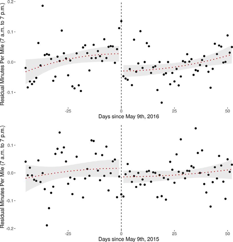
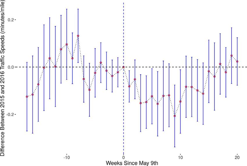
M. Tarduno Journal of Urban Economics 122 (2021) 103318

Fig. 3. Difference in Differences Results. Notes: Results from Eq. 1, a difference in differences comparing pre vs. post May 9th traffic speeds in 2015 (where both Uber
and Lyft operated in Austin) to pre vs. post May 9th traffic speeds in 2016 (where both TNCs exited Austin). Points represent the estimated effect of TNC departure
on traffic speeds (in minutes per mile) by hour of day. Controls include day of week, holiday, and segment fixed effects, segment-specific linear trends in days since
May 9th , and flexible controls for temperature and precipitation. Bars reflect 95% confidence intervals from two-way standard errors clustered by segment-week.
Traffic speed data were accessed through the City of Austin’s Open Data Portal.

TNCs account for 10% of vehicle trips, for example, this difference in Table 1
speeds implies a bias on the order of 0.003 minutes per mile—one to two Road segment summary statistics.
orders of magnitude smaller than my estimates of the impact of TNCs mean sd min max
on traffic speeds. To the extent that speed differences do generate bias,
 Average Speed (mph) 24.74 9.61 2.17 95.04
they will lead me to overstate improvements in traffic speeds resulting
 Minutes Per Mile 2.99 1.79 0.63 27.69
from a TNC ban. Segment Length 0.72 0.57 0.06 3.80
 Number samples 4.77 3.77 1.00 45.00
 Number of Lanes 4.70 0.91 2.00 7.00
6. Results and discussion
 Summary statistics for traffic data along 79 road segments in Austin, TX. Speed
 data reflect the average travel time for Bluetooth devices that move from origin
6.1. Traffic speeds
 sensor to destination sensor during a given 15-min interval. As described in
 Section 4, data are also filtered for outliers. Traffic speed data were accessed
 Across multiple specifications, I find evidence of modest increases
 through the City of Austin’s OpenData Portal.
in traffic speeds following the exit of Uber and Lyft. Results from my
preferred specification (Eq. 1) are displayed in Table 2 and Fig. 3. Point
estimates of changes in minutes per mile are largely negative, suggesting
reduced congestion after the exit of Uber and Lyft. While the 95% con-
fidence intervals for hour-specific estimates of changes in travel times The 2015 regresion discontinuity estimates a null effect, offering evi-
generally include zero, an F-test rejects the null hypothesis of ℎ = 0 ∀ℎ dence that the 2016 regression discontinuity results are not driven by
( < 0.0001). Although TNCs appear to negatively impact morning rush seasonal changes in traffic patterns.
hour conditions, I estimate little change in evening rush hour speeds. Table 4 shows the results from running versions of Eqs. 1 and 3,
The largest improvements in travel times following TNC exit come, sur- pooling across hours. The pooled difference in differences results suggest
prisingly, between 11 a.m. and 2 p.m. Point estimates for off-peak hours that on average, speeds increase by 0.026 minutes per mile ( = 0.15),
(8 p.m. to 6 a.m.) are small and straddle zero. This pattern could be a or roughly 0.9% following TNC exit. Consistent with the hour-specific
result of TNCs comprising a higher share of vehicles during the middle estimates, restricting the pooled DID analysis to daytime hours (7 a.m.
of the day than during peak hours. Additionally, evening rush hour ef- to 7 p.m.) generates larger estimates of speed increases following TNC
fects could be muted if TNC users are more likely to share cars during exit ( = −0.068, = 0.2). This coefficient translates to a 2.3% increase
the evening than they are during the morning and early afternoon. in daytime traffic speeds. Fig. 4 displays the raw speed data for daytime
 Fig. 6 and Table 3 display results from Eq. 3, a regression discontinu- traffic by week of year for my study window, and provides evidence of
ity by hour of day. These figures are qualitatively similar to, but larger the absence of pre-trends. Fig. 5 plots an event study version of Eq. 1,
in magnitude than the difference in differences results, suggesting that where separate treatment effects are estimated for each week. Consistent
the short-term impacts of TNC exit may be more pronounced than the with the growth of RideAustin and other Austin-area TNC alternatives
medium-term impacts. Fig. 7 plots residuals from a pooled regression through the second half of 2016, the event study shows the treatment
discontinuity performed on daytime traffic speeds in 2016 (when Uber effect decaying over time: 2016 traffic speeds are significantly lower
and Lyft exited) and 2015 (where both companies operated year-round). than those in 2015 for 10 weeks following the exit of Uber and Lyft, but

 6

M. Tarduno Journal of Urban Economics 122 (2021) 103318

 Fig. 4. Parallel Trends. Notes: This figure shows raw
 average speed (minutes per mile) between 7 a.m. and
 7 p.m. over 79 road segments in Austin, TX, plotted by
 week of year for 2015 and 2016. Data were accessed
 through the City of Austin’s Open Data Portal. The dot-
 ted line represents the week of May 9th , where Uber
 and Lyft ceased operation in Austin in 2016. Note that
 week zero is partially treated, as May 9th , 2016 was a
 Monday.

Fig. 5. Event Study. Notes: This figure plots results from a difference in differences regression with separate coefficients for 17 pre and 20 post-exit weeks. Points
represent the estimated difference between 2015 and 2016 traffic speeds (in minutes per mile) relative to the difference in the week leading up to May 9th . Controls
include day of week, holiday, SXSW, and segment fixed effects, as well as flexible controls for temperature and precipitation. Bars reflect 95% confidence intervals
from standard errors clustered by segment.

by week 17, point estimates suggest that traffic speeds had returned to data provide some insight into the level of alternative TNC activity in
the baseline 2015–2016 difference. Austin, it is unclear whether the growth of RideAustin in 2016 is repre-
 As in the hour-specific estimates, the pooled RD estimates are larger sentative of the growth of all alternative TNCs, or whether RideAustin
in magnitude than are the DID results: Travel times decreased by 0.102 grew by cutting into the market share of firms like Fasten and Fare,
minutes per mile ( = 0.01) across all hours and by 0.134 ( = 0.003) which arrived earlier. In Table 5, I report estimates of the impact of
minutes per mile for daytime hours. These coefficients correspond to TNCs on traffic speeds in Austin under each of these two possible trajec-
travel time reductions of 3.4% and 4.5%, respectively. tories of TNC activity in 2016: In rows 1 and 3 (RideAustin Data), I as-
 As noted in Section 3, a number of ridesharing firms entered the sume 10,200 TNC trips per day during the pre-period (see Uber (2015)),
market after the exit of Uber and Lyft. If alternative TNC activity was and use RideAustin’s time-series data—inflated by the reciprocal of its
substantial during the study period, my results will be attenuated rela- market share—to produce a time-varying measure of TNC activity fol-
tive to the counterfactual of a TNC-free Austin. Although RideAustin’s lowing the failure of Proposition 1. This time series is plotted in red in

 7

M. Tarduno Journal of Urban Economics 122 (2021) 103318

Fig. 6. Regression Discontinuity Results. Notes: Results from Eq. 3, a regression discontinuity performed on traffic speeds across 79 road segments in Austin, TX.
The bandwidth is March 20th - August 1st of 2016, which (asymmetrically) spans the May 9th departure of Uber and Lyft. Points represent the estimated effect of
TNC exit on traffic speeds by hour of day. A negative point indicates an estimated increase in traffic speed. Controls include day of week, holiday, and segment
fixed effects, segment-specific second degree polynomials in days since May 9th , and flexible controls for temperature and precipitation. Bars reflect 95% confidence
intervals from two-way standard errors clustered by segment-week. Traffic speed data were accessed through the City of Austin’s Open Data Portal.

 Table 3
Table 2
 Regression discontinuity results.
Difference in differences results.
 Hour of Day ℎ 
 Hour of Day ℎ 
 0 −0.0598 0.0297 0.0637
 0 −0.0606 0.0515 0.2588
 1 −0.0959 0.0343 0.0142
 1 −0.0525 0.0358 0.1640
 2 −0.0316 0.0251 0.2287
 2 −0.0505 0.0278 0.0908
 3 0.0202 0.0348 0.5711
 3 −0.0121 0.0649 0.8547
 4 0.0156 0.0690 0.8245
 4 0.0911 0.1006 0.3805
 5 −0.0920 0.0395 0.0352
 5 −0.0293 0.0920 0.7547
 6 −0.0267 0.0618 0.6727
 6 −0.0568 0.0996 0.5778
 7 −0.1081 0.1016 0.3050
 7 −0.1446 0.1169 0.2365
 8 −0.1370 0.1666 0.4248
 8 −0.0583 0.1331 0.6680
 9 −0.0661 0.0769 0.4047
 9 −0.0188 0.0954 0.8469
 10 0.0128 0.0566 0.8249
 10 0.0318 0.0581 0.5921
 11 −0.1137 0.0462 0.0275
 11 −0.1418 0.0664 0.0508
 12 −0.2675 0.0744 0.0029
 12 −0.1730 0.0812 0.0512
 13 −0.2861 0.0878 0.0057
 13 −0.1555 0.0927 0.1157
 14 −0.0932 0.0404 0.0368
 14 −0.0176 0.0469 0.7125
 15 −0.0759 0.0398 0.0775
 15 −0.0238 0.0453 0.6083
 16 −0.0187 0.0449 0.6833
 16 0.0657 0.0683 0.3524
 17 −0.0623 0.0561 0.2856
 17 0.0016 0.0591 0.9790
 18 −0.0257 0.0715 0.7246
 18 0.0500 0.0862 0.5715
 19 −0.0605 0.0539 0.2808
 19 −0.0300 0.0638 0.6451
 20 −0.0727 0.0565 0.2188
 20 0.0004 0.1036 0.9966
 21 −0.1082 0.1144 0.3601
 21 0.0817 0.0703 0.2646
 22 −0.1388 0.1126 0.2379
 22 −0.0709 0.0852 0.4191
 23 -0.0385 0.0544 0.4910
 23 −0.0152 0.0328 0.6497
 F-test 0.0000
 F-test 0.0000
 N 501,010
 N 966,301

Notes: Results from Eq. 1, a difference in differences comparing pre vs. post May Notes: Results from Eq. 3, a regression discontinuity performed on traffic speeds
 across 79 road segments in Austin, TX. The bandwidth is March 20th - August
9th traffic speeds in 2015 to pre vs. post May 9th traffic speeds in 2016 (where
 1st of 2016, which (asymmetrically) spans the May 9th departure of Uber and
both Uber and Lyft exited Austin). Controls include segment-specific linear in
day trends, a precipitation dummy, day of week fixed effects, and year and post Lyft. Controls include hour of day, day of week, holiday, and segment fixed
 effects, segment-specific second degree polynomials in days since May 9th , and
May 9th dummies. Standard errors are clustered by segment-week. ℎ represent
 flexible controls for temperature and precipitation. Standard errors are clustered
the estimated effect of TNC departure on traffic speeds (in minutes per mile)
by hour of day. Bold coefficients are significant at the 10% level. The final row by segment-week. ℎ represent the estimated effect of TNC departure on traffic
 speeds (in minutes per mile) by hour of day. Bold coefficients are significant at
reports the p-value from a joint hypothesis test of ℎ = 0 ∀ℎ.
 the 10% level. The final row reports the p-value from a joint hypothesis test of
 ℎ = 0 ∀ℎ.
 8

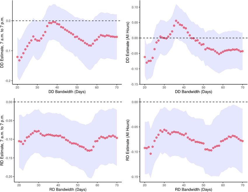
M. Tarduno Journal of Urban Economics 122 (2021) 103318

Fig. 7. Regression Discontinuity Residual Plots. Notes: This figure plots the daily mean residuals from a pooled version of Eq. 3, omitting the (year∗ post) indicator.
The dependent variable is minutes per mile, measured over 79 road segments in Austin, TX. The bandwidth is March 20th - August 1st of 2016 (or 2015), which
(asymmetrically) spans the May 9th departure of Uber and Lyft. Controls include hour of day, day of week, holiday, and segment fixed effects, segment-specific
second degree polynomials in days since May 9th , and flexible controls for precipitation and temperature. The dotted line represents a second degree polynomial in
days since May 9th ; the shaded region is the 95% confidence interval. Traffic speed data were accessed through the City of Austin’s Open Data Portal.

Fig. 2. Under this assumption, neither the fuzzy DID nor the fuzzy RD 7.6% reduction in travel speeds when moving from zero TNC activity
specification differs significantly from the results in Table 4. In rows 2 to full TNC activity—as an upper bound for the congestion impacts of
and 4 (Hampshire Data), I again use 10,200 TNC trips per day for the TNCs in Austin.
pre-exit figure, but then assume that a constant 4180 (41% of 10,200) My estimates of changes in traffic speeds together with data on the
TNC trips per day during are completed during the treatment period. number of total TNC and non-TNC vehicle trips in Austin allow me to
This figure reflects results from a November 2016 survey conducted by estimate the implied elasticity of congestion with respect to TNC vol-
Hampshire et al. (2017), where 41% of survey respondents reported that umes. According to the 2017 NHTS, Austin-area households take an av-
they completed an Uber or Lyft reference trip using another TNC follow- erage of 3.6 vehicle trips a day. Austin’s 37,000 households, then, gen-
ing the failure of Proposition 1. This trajectory assumes that RideAsutin’s erate roughly 1.35 million vehicle trips per day. The available data on
growth is not representative of the alternative TNC market, and instead Uber and Lyft suggest that the two services together completed roughly
entirely reflects RideAustin winning over customers from other already- 10,200 trips per day prior to their 2016 exit from Austin (see Fig. 2).
established Uber and Lyft alternatives. Multiplying this figure by a factor of two to reflect the capacity factor
 Intuitively, the results using the Hampshire Data assumption are estimated by Judd and Krueger (2016) suggests that Uber and Lyft to-
roughly 1.7 times larger than the estimates from Table 4. This of- gether accounted for 1.5% of Austin-area vehicle trips prior to the failure
fers a useful bound for this exercise investigating attenuation. If the of Proposition 1. My pooled estimates of the impact of TNCs on Austin-
RideAustin data is even partially representative of the growth of alterna- area congestion therefore imply congestion elasticities with respect to
tive ridesharing companies in Austin, then TNC activity in May–August TNC volume of between 0.6 and 2.3. My preferred specification, which
of 2016 was lower than the 41% replacement reported by Hampshire suggests a 2.3% increase in daytime traffic speeds following the exit of
et al. (2018) in November. I therefore view row 4—which implies a Uber and Lyft, corresponds to an elasticity 1.5. These estimates lie on

 9

M. Tarduno Journal of Urban Economics 122 (2021) 103318

 Fig. 8. Weekday vs. Weekend Effects. Notes: This figure plots
 difference in differences estimates (Eq. 1) of the impact of Uber
 and Lyft’s exit on travel speeds separately for weekdays and
 weekends. Points represent the estimated effect of TNC depar-
 ture on traffic speeds (in minutes per mile) by hour of day.
 Controls include day of week, holiday, and segment fixed ef-
 fects, segment-specific linear trends in days since May 9th , and
 flexible controls for temperature and precipitation. Bars re-
 flect 95% confidence intervals from two-way standard errors
 clustered by segment-week. Traffic speed data were accessed
 through the City of Austin’s Open Data Portal.

the lower end of the range of congestion elasticities from existing stud- shown in Fig. D.2. 5 of the 134 placebo coefficients (4%) fall below the
ies. Anderson et al. (2016), for example, estimate a congestion elasticity estimate using the true exit date, suggesting that it is empirically un-
of 2.7 in Beijing; findings from Leape (2006) imply an elasticity of 2.5 likely that my RD estimates are the result of an unobserved Austin-area
in London, and results from Eliasson (2009) imply an elasticity of 1.5 transit shock.
in Stockholm. The relatively small congestion elasticity implied by my
estimates may reflect the lower levels of congestion in Austin relative to 6.2. Heterogeneity and external validity
cities like London and Beijing, or the offsetting effect of trips saved by
the ‘ridesharing effect’ of TNCs. Results from Eq. 2, which allows for segment-specific congestion re-
 In Appendix D, I investigate the robustness of the results presented sponses, are plotted in Figs. 9 and 10. Two themes emerge. First, there is
in this section. Fig. D.1 plots both the difference in differences and re- no clear spatial pattern in congestion impacts: I estimate negative and
gression discontinuity results for bandwidths ranging from 20 to 70 days positive travel time impacts both for segments in the city center and
around May 9th . The conclusion that daytime traffic speeds increase fol- for outlying roads. Second, Fig. 9 shows that segments that experienced
lowing the exit of Uber and Lyft holds across bandwidth choices. To exceptionally large changes in traffic speed were characterized by ex-
test the likelihood that the regression discontinuity estimates presented ceptionally high levels of pre-period traffic congestion, suggesting con-
above are the result of a contemporaneous shock to Austin-area traf- struction or other segment-specific shocks may explain these estimates.
fic speeds, I compare my estimates to coefficients from 134 regression Absent these outliers, the segment-specific effects exhibit relatively low
discontinuities using placebo exit dates. The results of this exercise are variance. An important avenue for future work would be to investigate

 10

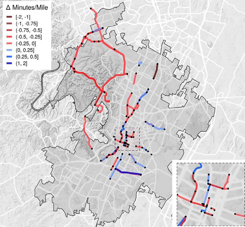
M. Tarduno Journal of Urban Economics 122 (2021) 103318

Fig. 9. Distribution of Segment-Specific Responses. Notes: Results from Eq. 2, a difference in differences comparing pre vs. post May 9th traffic speeds in 2015
(where both Uber and Lyft operated in Austin) to pre vs. post May 9th traffic speeds in 2016 (where both Uber and Lyft exited Austin), allowing for segment-specific
congestion responses. Bars represent the number of segments with idiosyncratic changes in traffic speeds falling withing a given bin. Cells are colored by the pre May
9th 2016 congestion level, as measured by the ratio of average speed to the 95th percentile of speed. Traffic speed data were accessed through the City of Austin’s
Open Data Portal.

 Fig. 10. Segment-Specific Responses. Notes: Results from
 Eq. 2, a difference in differences comparing pre vs. post
 May 9th traffic speeds in 2015 (where both Uber and Lyft
 operated in Austin) to pre vs. post May 9th traffic speeds
 in 2016 (where both Uber and Lyft exited Austin), allow-
 ing for segment-specific congestion responses. Paths rep-
 resent Google Maps recommended driving directions be-
 tween endpoints of a given segment, colored by the sign
 and magnitude of the estimated segment-specific change
 in traffic speed. The black line is the Austin city limit. Traf-
 fic speed data were accessed through the City of Austin’s
 OpenData Portal.

 11

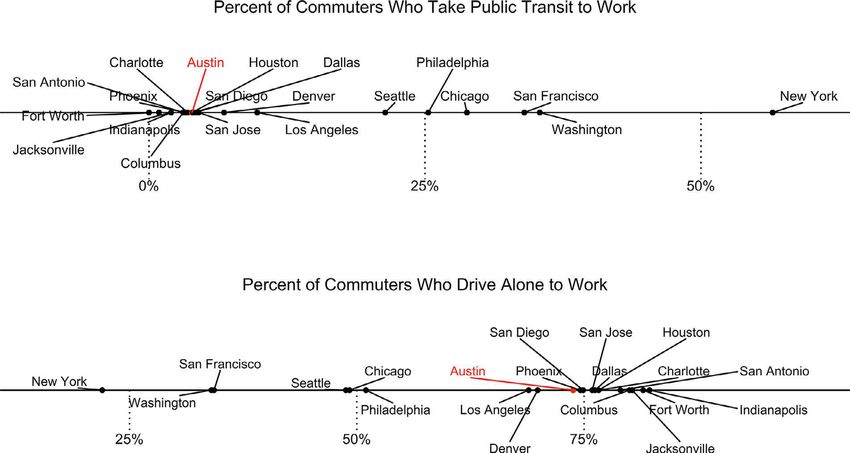
M. Tarduno Journal of Urban Economics 122 (2021) 103318

Fig. 11. External Validity. Notes: This figure depicts vehicle and public transit use across the 20 largest US cities for the year 2017. Data for both subfigures come
from the U.S. Census Bureaus 2017 American Community Survey. Similarities in commuting behavior between Austin and other “Sun Belt” cities suggests that the
findings in this paper may be most applicable to this group of metros.

 Table 4
 Pooled estimates.

 (Δ minutes/mile) Implied annual cost ($)

 Difference in Differences (All hours) −0.0261 0.0170 0.1479 −33,096,514
 Difference in Differences (7 a.m. - 7 p.m.) −0.0684 0.0529 0.2004 −63,985,000
 Regression Discontinuity (All Hours) −0.1015 0.0353 0.0052 −129,010,337
 Regression Discontinuity (7 a.m. - 7 p.m.) −0.1335 0.0433 0.0028 −124,930,327

 Notes: The first two rows display results from a variation of Eq. 1, a difference in differences specification that
 estimates the pooled impact of TNC exit on traffic speeds across hours of day. represent the estimated effect of
 TNC departure on traffic speeds, measured in minutes per mile. Controls include segment-specific linear in day
 trends, controls for precipitation, day of week fixed effects, hour of day fixed effects, and year and post-May
 9th dummies. Standard errors are clustered by segment-week. Row 1 shows the results of this regression using
 speed data on all hours, and column 2 shows results restricted to 7 a.m. to 7 p.m. The final column displays
 annual costs implied by multiplying by annual Ausin-area VMT, and then by $15.40, which is 50% of the
 average per-worker wage rate for Austin households, according to the 2017 NHTS. Traffic data were accessed
 through the City of Austin’s OpenData Portal. Rows 3 and 4 repeat this exercise for Eq. 3.

whether these outliers indeed represent extreme congestion reductions dition to the first-order changes in traffic flow caused by the absence
from TNC operation in select locations, or whether they can be explained of TNCs, the full equilibrium response to the exit of TNCs would reflect
by data absent from this setting. a combination of short and long-run adjustments made by road users.
 The external validity of the results presented in this paper hinges on More specifically, road users will spatially re-optimize in response to
whether Austin is representative of other metropolitan areas in terms of differential speed changes, and city residents may change long run by
commuter preferences and the substitutability of transit options. To de- vehicle purchase or sorting decisions.
termine which cities have transit systems that resemble Austin’s, Fig. 11 Because spatial re-optimization over route choices likely occurs in
depicts how public transit use and personal vehicle travel vary across the short-run, and I use a large sample of segments covering different
the 20 largest metro areas in the US. Commuters in the majority of large types of roadways, my estimates likely reflect this spatial substitution.
American cities (especially those located in the ‘Sun Belt’) exhibit mode My results do not, however, reflect long-term adjustments: The above
choices similar to those in Austin, where commuters heavily favor solo analysis compares traffic speeds in Austin with and without TNCs, hold-
commutes in personal vehicles. In cities with extensive public transit sys- ing fixed decisions on car purchasing behavior and locational sorting.
tems (e.g. New York, Washington, San Francisco), however, commuter Some of the reduction in congestion that I measure likely comes from
choices are quite different than they are in Austin. This suggests cau- individuals who, prior to 2016, chose not to purchase a vehicle because
tion when applying the results described in this paper to address policy they had access to ridesharing. In the long run, the actions of these
questions in these metro areas. marginal car owners would erode the traffic improvements that resulted
 from the exit of Uber and Lyft.
6.3. Equilibrium response
 6.4. Congestion costs
 It is worth discussing the extent to which the brief disruption of TNC
activity in Austin provides insights into the equilibrium differences in Armed with estimates of hour-specific changes in travel times, I cal-
congestion levels between a city with and a city without TNCs. In ad- culate the external congestion cost associated with TNC operation as

 12

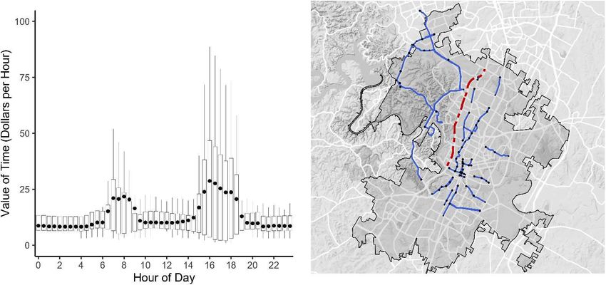
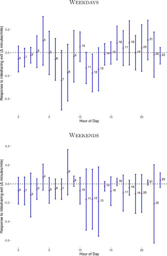
M. Tarduno Journal of Urban Economics 122 (2021) 103318

Table 5 Table 7
Fuzzy RD and Fuzzy DD. Congestion cost estimates.

 (Δ minutes/mile) Daily cost ($) annual cost ($)

 Fuzzy DID, RideAustin Data 0.0721 0.0573 0.2084 Time-varying VOT −92,071 97,547 0.1806 −33,605,827
 Fuzzy DID, Hampshire Data 0.0978 0.0237 0.0010 Uniform $15.40 VOT −127,983 72,156 0.0489 −46,713,725
 Fuzzy RD, RideAustin Data 0.1324 0.0133 0.0000
 Fuzzy RD, Hampshire Data 0.2263 0.0227 0.0000 Notes: Estimates of the travel-time congestion costs of TNC operation in Austin,
 TX. The first row displays the result of the exercise described in Eq. 4, which
Notes: The first two rows display results from a fuzzy difference in differences matches hour-specific changes in travel time to hour-specific willingness to pay
specification that estimates the impact of TNC activity on Austin traffic speeds estimates (detailed in Appendix A) and hour-specific traffic volume measure-
between 7 a.m. and 7 p.m. The regression coefficient represents the change ments. The second row uses a VOT of $15.40, which is 50% of the average
in travel times (in minutes per mile) resulting from a change from full TNC per-worker wage rate for car-commuting Austin households, according to the
operation [1] to no TNC operation [0]. The first row (RideAustin Data) uses 2017 NHTS. Standard errors for cost figures are calculated following Goodman
RideAustin’s trip-level data together with estimates of RideAustin’s market share (1960). See Table 8 for hour-by-hour cost estimates.
to construct a measure of daily TNC activity. The second row assumes that the
level of TNC activity during the period following the exit of Uber and Lyft was
a constant 41% of pre-exit levels. This assumtion is based on a November 2016
survey conducted by Hampshire et al. (2018). Rows three and four report results million (p=0.049). Disaggregating this sum by weekend and weekday
from fuzzy regression discontinuity designs that estimate the impact of TNC effects (Table 9) produces slightly larger figures annual cost figures:
activity on Austin traffic speeds between 7 a.m. and 7 p.m., using the same TNC $39 million (p=0.041) and $52 million (p=0.003). In Appendix D, I re-
activity assumptions. port results from this exercise using a regression where observations are
 weighted by the number of Bluetooth devices recorded in each 15-min
follows: window. The rationale for this specification is to investigate whether
 ∑ the above results are biased when segments with differing traffic flows
Δcongestion cost = Δ minutes per mileℎ ∗ miles drivenℎ ∗ value of timeℎ are implicitly given the same weight in determining regression coeffi-
 ℎ
 cients. The cost estimates from this weighted regression are similar to
 (4)
 the non-weighted results and imply an annual congestion cost associ-
Δ minutes per mile are the coefficients, by hour of day, ℎ, estimated ated with Austin-area TNC activity of $54 million. Note that each of
above. To estimate miles drivenℎ , I use periodic traffic counts to estimate these aggregate cost measures relies on the assumption that VOT is uni-
the share of VMT by hour of day in Austin, and multiply these shares form across the city. While misattributing VOT estimates by location
by estimates of daily VMT provided by the Texas Department of Trans- may bias these estimates, there are two reasons why this bias is likely
portation. Note that this operation assumes that my estimates represent small: First, in a recent investigation of the heterogeneity of urban VOT,
an average effect for all VMT within Austin City limits. Table 6 provides Buchholz et al. (2020) find that the majority of the variation in VOT
evidence in support of this assumption: According to data maintained by is across individuals rather than across locations within a city. Second,
the Texas Department of Transportation, roads included in my preferred the lack of a spatial gradient in the segment-level congestion estimates
specification resemble those not included in terms of congestion, VMT, (see Fig. 10) means that a cost calculation using a modest VOT gradient
and speed. Finally, I calculate Austin-specific hourly value of travel time between the city and the suburbs (as in Fig. 8 of Buchholz et al. (2020))
(VOT) estimates (value of timeℎ , above) using data from Austin’s MoPac would produce similar aggregate welfare measures as those reported
freeway (see Appendix A). I also present results using a VOT heuris- above in Tables 4 and 7, so long as the VOT estimates I use reflect the
tic from Small and Verhoef (2007): 50% of the wage rate. I estimate rough spatial average of the Austin metro area.
the wages of Austin-area drivers by calculating the per-worker income Several outside studies provide valuable context when interpreting
for car-commuting Austin households in the 2017 National Household these congestion cost estimates. First, according to the Inrix Global
Travel Survey (NHTS). Standard errors for all congestion cost estimates Scorecard, the aggregate 2017 travel time cost in Austin was $2.8
follow formulas developed by Goodman (1960). billion, $810 million of which was attributed to traffic slowdowns
 I report the results of this exercise in Table 7. Both rows reflect (Inrix, 2017). Back of the envelope calculations using my estimates
changes in travel times estimated in my preferred specification (Eq. 1), therefore suggest that Uber and Lyft together accounted for 1–2% of all
a DID across years. Using time-varying (MoPac) and uniform (NHTS) travel time costs in Austin, and 4–6% of congestion costs. Second, esti-
VOT estimates, I calculate the daily congestion costs associated with mates of consumer surplus associated with TNCs offer a useful bench-
Uber and Lyft activity at $92,071 and $127,983, respectively. These es- mark for policymakers weighing the benefits of TNC operation against
timates correspond to annual costs of $33 million (p=0.181) and $46 the costs. The results from Cohen et al. (2016) allow me to produce two

 Table 6
 Austin metro validity.

 Not Sampled Sampled p

 Annual Delay per Mile (person-hours) 118,372.98 101,368.11 0.58
 Texas Congestion Index 1.36 1.39 0.61
 Peak Period Average Speed 33.22 29.52 0.16
 Freeflow Speed 41.20 37.97 0.28
 Average Daily VMT 204,488.84 166,805.50 0.46
 Peak Period Annual Hours of Delay (person-hours) 377,230.86 241,909.86 0.34

 Notes: This table uses data maintained by the Texas Department of Transportation (TXDoT)
 to compare observable characteristics of Austin-area roads that do not appear in my sample
 (column 1) to those that do (column 2). Column (3) reports p-value of the corresponding
 t-test for a difference in means. The data cover 86 road segments in Austin, 35 of which
 overlap with the 79 Bluetooth segments used in the above analysis. Note that roads sections
 are coded as sampled even if the Bluetooth segment does not cover the entire corresponding
 TXDoT road segment.

 13