Time-Scales of Inter-Eruptive Volcano Uplift Signals: Three Sisters Volcanic Center, Oregon (United States) - E-Prints ...
←
→
Page content transcription
If your browser does not render page correctly, please read the page content below
ORIGINAL RESEARCH
                                                                                                                                             published: 21 January 2021
                                                                                                                                         doi: 10.3389/feart.2020.577588

                                            Time-Scales of Inter-Eruptive Volcano
                                            Uplift Signals: Three Sisters Volcanic
                                            Center, Oregon (United States)
                                            Sara Rodríguez-Molina 1, Pablo J. González 2,3*, María Charco 1, Ana M. Negredo 1,4 and
                                            David A. Schmidt 5
                                            1
                                              Institute of Geosciences (IGEO, CSIC, UCM), Madrid, Spain, 2COMET, Department of Earth, Ocean and Ecological Sciences,
                                            School of Environmental Sciences, University of Liverpool, Liverpool, United Kingdom, 3Volcanology Research Group,
                                            Department of Life and Earth Sciences, Institute of Natural Products and Agrobiology (IPNA-CSIC), La Laguna, Spain,
                                            4
                                              Department of Earth Physics and Astrophysics, Faculty of Physical Sciences, Complutense University of Madrid, Madrid, Spain,
                                            5
                                              Department of Earth and Space Sciences, University of Washington, Seattle, WA, United States

                                            A classical inflation-eruption-deflation cycle of a volcano is useful to conceptualize the time-
                                            evolving deformation of volcanic systems. Such a model predicts accelerated uplift during
                                            pre-eruptive periods, followed by subsidence during the co-eruptive stage. Some
                                            volcanoes show puzzling persistent uplift signals with minor or no other geophysical or
                             Edited by:     geochemical variations, which are difficult to interpret. Such temporal behaviors are usually
                       Flavio Cannavo’,
      National Institute of Geophysics      observed in large calderas (e.g., Yellowstone, Long Valley, Campi Flegrei, Rabaul), but less
                      and Volcanology,      commonly for stratovolcanoes. Volcano deformation needs to be better understood during
              Section of Catania, Italy
                                            inter-eruptive stages, to assess its value as a tool for forecasting eruptions and to
                        Reviewed by:
                                            understand the processes governing the unrest behavior. Here, we analyze inter-
                     Maurizio Battaglia,
     United States Geological Survey        eruptive uplift signals at Three Sisters, a complex stratovolcano in Oregon
                (USGS), United States       (United States), which in recent decades shows persistent inter-eruptive uplift signals
                  Gilda Maria Currenti,
      Istituto Nazionale di Geofisica e
                                            without associated eruptive activity. Using a Bayesian inversion method, we re-assessed
              Vulcanologia (INGV), Italy    the source characteristics (magmatic system geometry and location) and its uncertainties.
                  *Correspondence:          Furthermore, we evaluate the most recent evolution of the surface deformation signals
                    Pablo J. González
                                            combining both GPS and InSAR data through a new non-subjective linear regularization
              pjgonzal@liverpool.ac.uk
                                            inversion procedure to estimate the 26 years-long time-series. Our results constrain the
                    Specialty section:      onset of the Three Sisters volcano inflation to be between October 1998 and August 1999.
         This article was submitted to      In the absence of new magmatic inputs, we estimate a continuous uplift signal, at
                          Volcanology,
               a section of the journal     diminishing but detectable rates, to last for few decades. The observed uplift decay
            Frontiers in Earth Science      observed at Three Sisters is consistent with a viscoelastic response of the crust, with
          Received: 29 June 2020            viscosity of ∼1018 Pa s around a magmatic source with a pressure change which increases
      Accepted: 23 November 2020
                                            in finite time to a constant value. Finally, we compare Three Sisters volcano time series with
       Published: 21 January 2021
                                            historical uplift at different volcanic systems. Proper modeling of scaled inflation time series
                              Citation:
    Rodríguez-Molina S, González PJ,        indicates a unique and well-defined exponential decay in temporal behavior. Such
         Charco M, Negredo AM and           evidence supports that this common temporal evolution of uplift rates could be a
   Schmidt DA (2021) Time-Scales of
 Inter-Eruptive Volcano Uplift Signals:     potential indicator of a rather reduced set of physical processes behind inter-eruptive
Three Sisters Volcanic Center, Oregon       uplift signals.
                       (United States).
           Front. Earth Sci. 8:577588.      Keywords: inter-eruptive deformation, characteristic relaxation time, continuous GPS, interferometric synthetic
      doi: 10.3389/feart.2020.577588        aperture radar, geodetic time series, Three Sisters volcano

Frontiers in Earth Science | www.frontiersin.org                                    1                                          January 2021 | Volume 8 | Article 577588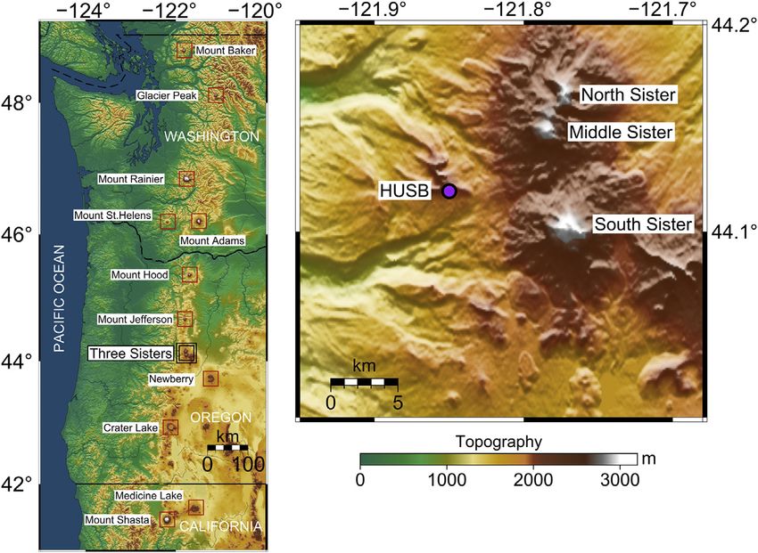
Rodríguez-Molina et al.                                                                                      Inter-Eruptive Volcano Uplift Time-Scales

1 INTRODUCTION                                                             known examples of uplifting volcanoes to understand 1) whether
                                                                           a variety or not of physical mechanism are at work behind
Many volcanoes follow a common deformation pattern                         deformation and, if so, 2) if uplift time-scales are informative
consisting of uplift during inter-eruptive periods and                     of whether a certain volcano is on a late or early stage of the inter-
subsidence in co-eruptive stages, occasionally interrupted by              eruptive period.
periods of quiescence or subsidence. Some other volcanoes do
not however exhibit this simple behavior (Biggs and Pritchard,
2017). Part of them show puzzling non-steady persistent uplift             2 BACKGROUND
signals that can last from days to years with minor or no other
geophysical or geochemical variations, which are difficult to               The Three Sisters Volcanic Complex forms a N-S chain of
interpret. Therefore, uplift during inter-eruptive episodes                stratovolcanoes located at 44.1+ N in the central Oregon
cannot be only interpreted as a pre-eruptive precursory                    Cascades (Figure 1), an active volcanic arc produced by the
indicator. Such temporal behavior is usually observed in large             subduction of the Juan de Fuca and Gorda plates beneath the
calderas (e.g., Yellowstone, Long Valley, Campi Flegrei, Rabaul),          North American plate. In addition to this convergent motion,
but less commonly for stratovolcanoes.                                     there is an oblique relative plate motion and northward push of
   An important goal in volcano eruption forecasting is to find             the Sierra Nevada-Great Basin microplate, favoring a N-S stress
how the deformation time-series can distinguish among physical             orientation of the vents within the Oregon Cascades (Mccaffrey
processes, especially during inter-eruptive periods leading to a           et al., 2007). South Sisters is near the propagating tip of a crustal
pre-eruptive scenario. The latter are characterized by new                 melting anomaly westward across Oregon, progressing since the
injections of magma/increment of volatiles, viscoelastic                   mid-Miocene, going through the Cascades in the Quaternary
relaxation of the media, or a mixing of different coeval                   (Fierstein et al., 2011). All these circumstances influence on the
processes. Therefore, we must constrain what controls usually              eruptive history of Three Sisters.
long-lived or persistent uplift at volcanic centers. Le Mével et al.           The Three Sister area includes shields, composite volcanoes
(2015) show that the temporal evolution of deformation                     and cinder cones, with basaltic to rhyolitic volcanism. The three
surprisingly follows the same pattern for different volcanic               eponymous volcanoes are progressively younger from north to
systems at specific analyzed periods (Yellowstone, Long Valley,             south and exhibit little family resemblance (Hildreth et al., 2012).
Laguna de Maule and Three Sisters). This is consistent with the            North Sister is a monotonously mafic edifice created 120 ka ago,
hypothesis that similar processes may be at work in similar                formed by long-lived effusive volcanism (Schmidt and Grunder,
volcanoes. After this stage, these volcanoes presented an                  2011); Middle Sister is an andesite-basalt-dacite cone constructed
eventual pause and/or change to subsidence (related to seismic             between 48 ka and 14 ka and South Sister is a bimodal rhyolitic-
events and/or hydrothermal changes), but did not produce an                intermediate edifice built between 50 ka and 2 ka, both with
eruption.                                                                  histories of explosive volcanism (Scott et al., 2001). However,
   Stratovolcano behavior contrasts with better documented                 most of the volcanic activity is identified with mafic shields and
restless calderas (Acocella et al., 2015; Galetto et al., 2017).           cones around the major composite volcanoes (Hildreth, 2007).
Calderas usually show long repose periods between large                    Geochemical anomalies suggest that episodes of intrusion may be
eruptions, but without quiescence (e.g., resurgent volcanism,              more frequent in the Three Sisters area than the age of eruptive
subsidence, multiple pulses of uplift) (Biggs and Pritchard,               vents would involve (Evans et al., 2004). The most recent
2017). The Three Sisters complex volcano is a good example                 eruptions were rhyolitic close to South Sisters, 2000 years ago
of a system with long lasting monotonous inter-eruptive uplift             (Hildreth et al., 2012). There is a potential volcanic hazards threat
without associated eruptive activity or significant seismicity and          if future eruptions are similar to South Sister’s recent past. Tephra
might correspond with different magmatic system behaviors.                 fallout might accumulate to 1–2 cm thick in the Bend area, and
   In this work, we studied the decadal deformation time-series of         small-volume lahars and pyroclastic flows could pose a hazard to
the Three Sisters volcano in order to understand the processes             nearby areas (Sherrod et al., 2004).
governing its unrest behavior and to find out whether it is still               Before 2001, Three Sisters was considered a dormant volcano.
inflating. For this purpose, we needed to perform a consistent              Nonetheless, ERS-1/2 satellite interferometric synthetic aperture
analysis of the volume change time-series underlying the Three             data (InSAR) analysis from 1992 to 2000 revealed active uplifting
Sisters uplift signal, which is a challenging task. We analyze             located 6 km west of South Sister (Wicks, 2002). Geodetic
available continuous GPS data since 2001 and multiple                      information for Three Sisters volcanic center has been
satellite interferometric data spanning the 1993–2020 period.              accumulating since this discovery. Nowadays, deformation is
We proposed combining multiple geodetic data-sets using an                 continuously monitored through Leveling surveys since 2002,
improved linear regularization method based on Truncated                   Continuous GPS (CGPS), GPS campaign since 2001 and Semi
Singular Value Decomposition (TSVD) (González et al., 2013)                Permanent GPS (SPGPS) since 2009 (Dzurisin et al., 2009;
to find an optimal regularization criteria for Three Sister data-set        Dzurisin et al., 2017). The uplift at Three Sisters has been
combination. We obtained a seamless, continuous time series of             aseismic except for a swarm of ∼300 small earthquakes (Mmax
volume change (and its uncertainties) with which to rigorously             1.9) in March 2004 (Moran, 2004; Dzurisin et al., 2009). Previous
assess changes over the 26-years studied period. Finally, we               studies (Wicks, 2002; Dzurisin et al., 2006; Dzurisin et al., 2009;
compared the Three Sisters temporal behavior to other well-                Riddick and Schmidt, 2011) show evidence that observed uplift

Frontiers in Earth Science | www.frontiersin.org                       2                                    January 2021 | Volume 8 | Article 577588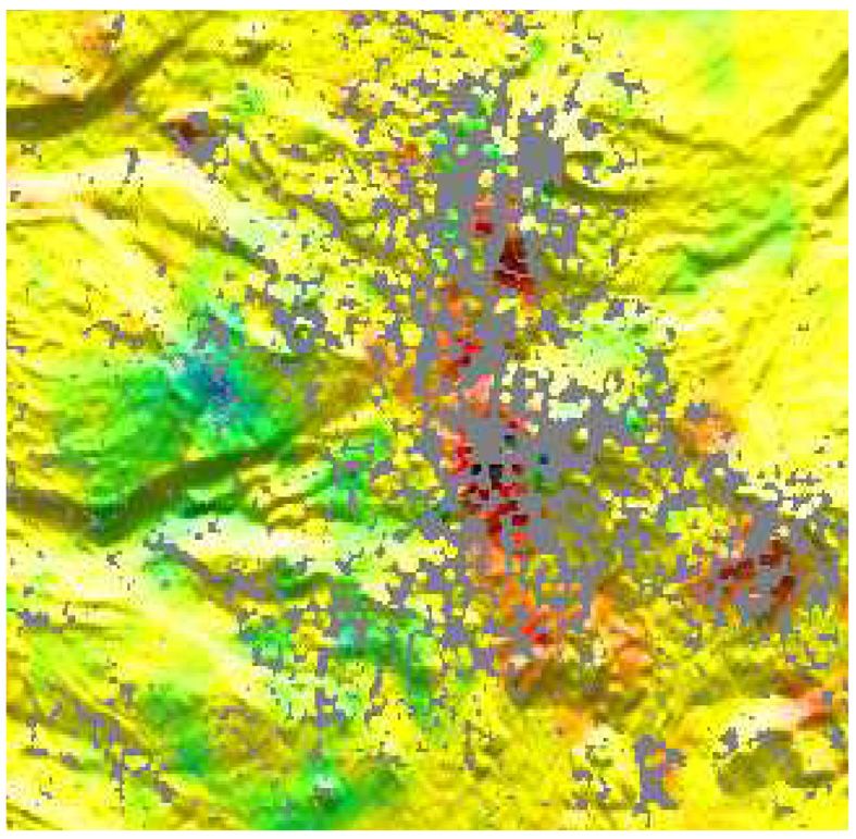
Rodríguez-Molina et al.                                                                                                      Inter-Eruptive Volcano Uplift Time-Scales

  FIGURE 1 | (A) Shaded relief map for the Cascade range, with locations of representative Cascade volcanoes. Three sisters volcano is highlighted with black
  squares. (B) Regional map of Three Sisters volcano complex. The continuous GPS station HUSB, located at ∼5 km west of South Sister volcano, is shown as a purple
  circle with black outline.

can be described by a spherical point source within an                                series is particularly important to understand the surface
homogeneous isotropic elastic half-space. Nevertheless,                               deformation time-scales at Three Sisters.
deformation source geometry is non-unique and sources as                                 Daily GPS data (coordinates and their uncertainties) are
horizontal crack, vertical prolate spheroid, and sill-like have                       analyzed by the USGS using GIPSY/OASIS II software.
been proposed at Three Sisters to fit geodetic data.                                   Common-mode daily biases are estimated and removed using
Interpretation of the temporal evolution of InSAR, leveling                           QOCA (Dzurisin et al., 2009). Three Sisters is located near the
and GPS data suggests the beginning of deformation in late                            actively deforming Cascadia margin, so any geodetic data and
1997 or 1998, with a maximum uplifting rate of 3-5 cm/year                            coordinates must consider the wider regional deformation
during 1998–2001. Microgravity data collected between 2002                            patterns. The motion of a background steady rigid-body with
and 2009 show no significant change in the mass flux across the                         a rotation pole situated near the eastern limit of Oregon must
deforming area (Zurek et al., 2012). No studies have been                             therefore be removed from the time-series, and a correction for
published about the uplift evolution over the last decade. The                        predicted horizontal tectonic motion should be applied. Here, we
uplift process was still on-going in January 2020, when this                          remove a linear trend of 4.29 mm/yr for the North component
manuscript was prepared.                                                              and 1.50 mm/yr for the East component. This model prediction
                                                                                      represents an update and improved version of the horizontal
                                                                                      displacements at HUSB (Dzurisin et al., 2006; Dzurisin et al.,
3 GEODETIC DATA PROCESSING                                                            2009; M. Lisowsky personal communication; Cascades Volcano
                                                                                      Observatory, 2017).
We aim to extend the detailed uplift history at Three Sisters                            Figure 2 shows the resulting GPS displacements between July
already mentioned above to the present (2020) by using the                            2001 and January 2020. CGPS data reveals several gaps that
available CGPS and InSAR data-sets.                                                   occurred due to snowfall in the winter seasons. Furthermore,
                                                                                      CGPS shows a gap and a posterior data offset during August
3.1 Continuous GPS                                                                    2017-August 2018. USGS data site reports some readjustment of
In May 2001, the U.S Geological Survey (USGS), in collaboration                       HUSB permanent station during this period and these could
with the U.S. Forest Service, installed a continuous GPS station                      explain some of the gaps and offsets in the time series.
(HUSB) near the actively deforming area. It was strategically
installed at a location approximately ∼2 km northwest of the
detected uplift center. HUSB is part of the USGS Pacific                               3.2 Interferometric Synthetic Aperture
Northwest Network, so it is automatically processed to obtain                         Radar (InSAR)
daily coordinates. No other regional and local continuous GPS                         Our InSAR data set includes 85 interferometric pairs, with
station falls within the deformation area. Hence, the HUSB time-                      temporal baselines from 35 to 2,894 days, from four satellite

Frontiers in Earth Science | www.frontiersin.org                                  3                                         January 2021 | Volume 8 | Article 577588
Rodríguez-Molina et al.                                                                                                     Inter-Eruptive Volcano Uplift Time-Scales

  FIGURE 2 | North (UNorth), east (UEast) and vertical (Uup) components of the continuous GPS displacements at HUSB.

missions (ERS, ENVISAT, ALOS-1 and Sentinel-1). ERS and
ENVISAT SAR images were acquired during summer and fall
between 1993 and 2010 (descending orbits, tracks 113 and 385;
ERS and ENVISAT look angles 20.2° and 19.8°, respectively). We
used 51 interferograms processed with the ROI PAC software
(Rosen et al., 2004) and unwrapped using SNAPHU (Chen and
Zebker, 2002), with perpendicular baselines up to 500 m, as
explained by Riddick and Schmidt (2011).
   To improve the temporal coverage of InSAR observations,
we also analyzed data from the ALOS-1 and Sentinel-1 SAR
data missions. The mean line-of-sight velocity of ALOS-1 data
(path 219, ascending orbit, look angle 38.7°) was obtained
during January 2007- March 2011. Most individual
interferograms in the Cascades range show poor coherence
because of vegetation and seasonal snow coverage, hence we
also processed 4 Sentinel-1 summer-to-summer and summer-
to-late spring interferometric pairs, between September 2015
and May 2018, for descending (path 115, look angle 39.8°) and
ascending (path 137, look angle 38.8°) orbits. To provide
deformation data during the GPS gap mentioned above,
two Sentinel-1 interferometric pairs cover that period. We
used JPL InSAR Scientific Computing Environment (ISCE)
software (Rosen et al., 2012), processing Level-0 raw ERS-1
and ALOS-1, and SLC-level Sentinel-1 radar data. All                                 FIGURE 3 | The linear surface deformation LOS velocity (mm/year)
                                                                                     obtained for the ascending Path 219 ALOS-1, using the small baselines
interferograms were corrected for orbital and topographic
                                                                                     method implemented in StaMPS (Hooper et al., 2012) for the period January
contributions using precise orbit information and the SRTM                           2007 to March 2011. Positive LOS velocity values corresponds to
digital elevation model (Farr et al., 2007). We also reprocessed                     displacements toward the satellite, i. e., uplifting. Black triangles and star
a highly coherent interferometric pair for ERS-1 track 365                           represent the Three Sister complex volcano system and the approximate
(descending orbit, corresponding to August 1997 - September                          center of the uplifting area. StaMPS LOS velocity results were noisy and we
                                                                                     post-processed to reduce undesirable oscillations of non-volcanic origin. We
2000). This interferogram was essential to further re-evaluate                       applied a band pass filter to retain spatial deformation signals between 10 and
the magmatic source location and constrain its uncertainties.                        0.8 km using a median filter (GMT blockmedian). Results indicate a 6 km
   L-band data (wavelength ∼24 cm) from ALOS-1 were very                             circular uplift pattern west of South Sister with a mean LOS velocity of
useful to avoid decorrelation owing to the vegetation                                approximately 5–10 mm/year, consistent with a value obtained for the
encompassing the Three Sisters area. Although the LOS                                Husband CGPS station during the same period (5.21 mm/year), shown as
                                                                                     circle with a black outline.
deformation rate from 2006 to 2010 is small (about 6–8 mm/yr)

Frontiers in Earth Science | www.frontiersin.org                                4                                          January 2021 | Volume 8 | Article 577588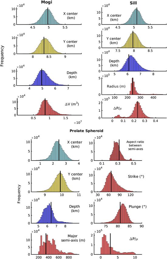
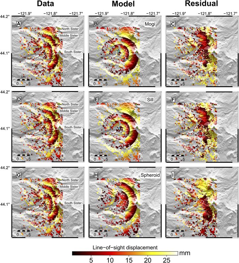
Rodríguez-Molina et al.                                                                                                         Inter-Eruptive Volcano Uplift Time-Scales

  FIGURE 4 | Wrapped InSAR data and model results for Track 385 of the ERS satellite. (A, D, G) Line-of-sight (LOS) deformation observed in a nearly 3 years period
  from August 24, 1997 and September 17, 2000, considering only pixels with coherence >0.2. Green triangles represent the Three Sister complex volcano system. (B, E,
  H) Bayesian model and horizontal location for the median a posteriori probability solution (blue star) for a predicted Mogi, sill-like and prolate spheroid source,
  respectively. (C, F, I) Residual maps for Mogi, sill-like and prolate spheroid source. The model parameters results are presented in Figure 5 and Tables 1, 2.

Frontiers in Earth Science | www.frontiersin.org                                   5                                          January 2021 | Volume 8 | Article 577588
Rodríguez-Molina et al.                                                                                             Inter-Eruptive Volcano Uplift Time-Scales

making it difficult for a single L-band interferogram to detect the               of the TSVD technique used to regularize the inverse problem,
deformation signal (Riddick and Schmidt, 2011), a cumulative LOS                 with the goal of finding the time evolution of volume and
deformation time-series can detect such changes in rate. The                     therefore to improve the accuracy on the estimation of volume
corresponding time-series was processed by StaMPS Version                        time series. First, we show how the active source location
3.3.b1 to study the surface deformation, applying the Small                      (horizontal position and depth) and geometry is determined
Baselines method for 30 interferometric pairs (Hooper et al.,                    using a Bayesian inversion approach. Subsequently, we solve
2012; Bekaert et al., 2017). Small Baselines method minimizes                    for temporal evolution of volume.
decorrelation in natural terrains. So, it is an appropriate method for
the Three Sisters area, which lacks man-made structures and hence                4.1 Source Characterization
offers few dominant persistent scatterers.                                       First of all, we infer the active magmatic source through a Bayesian
    Due to the small deformation rate (5.8 mm/year for the period                inversion, using InSAR data spanning the period of maximum
June 2015 - January 2020) and low signal-noise ratio in the                      displacement. The horizontal location, depth and geometry of the
Cascades, geodetic data must be analyzed carefully (Poland et al.,               inflation source at Three Sisters were computed using the
2017). Following this recommendation, we consider a 1 cm                         MATLAB®-based software package GBIS (Geodetic Bayesian
standard deviation for neighboring pixels in all interferograms.                 Inversion Software) (Bagnardi and Hooper, 2018), which
Only four good quality interferometric pairs were used for the                   estimates source parameters through a Markov chain Monte
Sentinel-1 observation period. Adding more interferograms did                    Carlo method and uses, among others, analytical forward models
not significantly improve the analysis of the volume change time-                 from dMODELS software package (Battaglia et al., 2013). It obtains
series. Moreover, the analysis of a 6-years long Sentinel-1 dataset              the posterior probability distributions (PDFs) for all model
in Turkey indicates that surface displacement rate uncertainties                 parameters by taking into account uncertainties in the data (e.g.,
are mostly dominated by length of observation, rather than larger                data errors). To achieve this, considering the pattern of surface
numbers of available interferograms (Weiss et al., 2020). Hence,                 deformation, we employ simple elastic models such as point source
we consider Sentinel-1 summer-to-summer and summer-to-late                       (Mogi, 1958), prolate spheroid (Yang et al., 1988) and sill-like (Fialko
spring InSAR data to avoid decorrelation due to snow coverage,                   et al., 2001) models. An elastic, homogeneous and isotropic half-
and to fill a noticeable GPS time-series gap. However, the                        space is assumed in all the approaches with Poisson’s ratio 0.25. We
deformation rates could be reexamined in future, using longer                    assumed, as previous studies (Dzurisin et al., 2006, 2009; Riddick and
Sentinel-1 datasets.                                                             Schmidt, 2011), a stationary source and we used an interferogram
    Figure 3 represents the mean LOS velocity (mm/year) for the                  spanning August 1997 - September 2000 to look for source
ascending path 219 ALOS-1 from January 2007 to March 2011. Due                   parameters. This interferogram fulfills two important conditions
to the high signal-to-noise ratio, the StaMPS LOS velocity results               to determine the best-fitting static displacements: 1) it spans the
were noisy and we post-processed them to reduce undesirable                      shortest time during the period of maximum deformation; 2) it
oscillations of non-volcanic origin. We applied a band pass filter                shows acceptable signal-to-noise ratio. InSAR spatially correlated
to retain spatial deformation signals between 10 and 0.8 km, using a             error (caused mainly by the “wet” tropospheric delay) is estimated by
median filter (GMT blockmedian). Although close to the signal-to-                 modeling experimental semivariograms in deformation-free regions
noise ratio value, results indicate a 6 km circular uplift pattern west of       (Bagnardi and Hooper, 2018). InSAR data are subsampled with an
South Sister with a mean LOS velocity of ∼5–10 mm/year. This                     adaptative quadtree method (Decriem et al., 2010) to reduce the
mean velocity is consistent with a value obtained for the HUSB                   computational cost of the Bayesian inversion, particularly for sill-like
CGPS station during the same period (5.2 mm/year).                               and prolate spheroid sources. The inversion computes 2×10⁶
                                                                                 iterations for spherical point source, 5×10⁶ iterations for sill-like
                                                                                 source and 8×10⁶ iterations for prolate spheroid, which stabilizes the
4 METHODS                                                                        inversion procedure.

Here, we introduce a mathematically rigorous strategy for the
joint inversion of time-dependent InSAR (different look angles                   4.2 Temporal Evolution of the Source
and sensors, high spatial resolution) and continuous GPS (daily                  Volume Changes
sampling) data to achieve a complete timeline of volcanic activity               Once the magmatic source is fixed, we perform the quasi-
and quantify a single time series of volume flux rates. The strategy              dynamic time-dependent model using a linear inversion
captures the benefits of each system avoiding the time evolution                  scheme to look for the volume changes at each interferogram’s
determination on a point-by-point basis. It is based on the two-                 period and the cumulative volume changes since the first GPS
step approach proposed by González et al. (2013) that produces                   observation. Both volume changes at each interferogram and
time series of volume from sets of different look angles and                     cumulative volume changes from the GPS data are used to solve
satellite sensors once an active source is determined for an                     for the time evolution of volume using TSVD.
inflation period. In this section, we provide a description of
the González et al. (2013) algorithm and extent it 1) to                         4.2.1 First Step: Piecewise Volume Changes Over
include continuous GPS data and therefore to combine                             Temporal Data Periods
different components and/or look vectors using a unique                          Once the location and geometry of the inflation source are fixed,
source model and 2) to afford a defined method of truncation                      we determine the volume changes over the corresponding time

Frontiers in Earth Science | www.frontiersin.org                             6                                     January 2021 | Volume 8 | Article 577588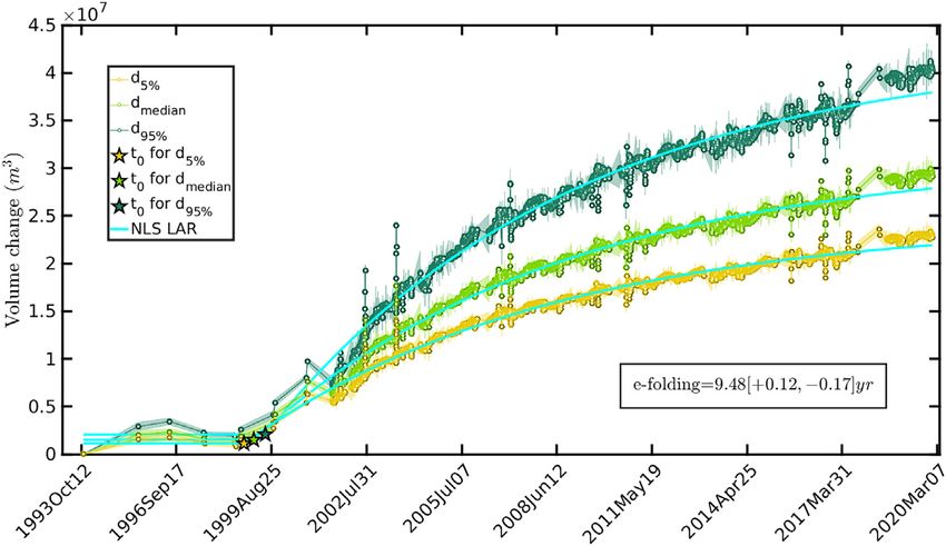
Rodríguez-Molina et al. Inter-Eruptive Volcano Uplift Time-Scales
intervals (increments of volume changes, ΔV) for both, InSAR BV_ ΔV, (3)
and CGPS data sets, which are assumed to be uncorrelated. In this
way, observations from several interferograms and GPS sites can where B is the design matrix (N × M). To determine the
be combined to estimate increments of volume changes assuming components of B, we define a (M × 1) vector E, containing
a unique source model. Each volume change, ΔVij , records 1) the the single epochs tj present in all time intervals and sorted in
incremental volume change between two acquisition dates, ti and chronological order, for j 1, ..., M; and a (N × 2) vector F, whose
tj from an interferogram or 2) the cumulative increment of columns are the slave (tslavei) and master (tmasteri ) epochs of each i
volume since the first observation, i.e., tj t0, being t0 the time interval, for i 1, ..., N. Therefore, the (i, j) component of the
starting date of CGPS. design matrix is Bij (tj+1 − tj) for tslavei ≤ tj < tmasteri , and zero
A linear inversion scheme using Weighted Least Squares elsewhere. In the case of cumulative ΔV (i.e., continuous GPS), B
(WLS, Menke, 1989) is applied. The inversion is constrained presents lower triangular matrix blocks. For example, if volume
by 55 interferometric pairs (ERS, ENVISAT, Sentinel-1), one changes are obtained over different time intervals, i.e., if tAB, tBC,
ALOS-1 interferogram (cumulative LOS deformation time- and tAC (from InSAR data), and tCD, tCE, tCF, (from CGPS data)
series) and a 3-component GPS time series. The forward are ΔvAB , ΔvBC , ΔvAC , ΔvCD , ΔvCE and ΔvCF , the design matrix is
problem is defined by d Gm, where d is the data vector given by:
(InSAR or GPS), m is the model parameter (ΔV) vector, and (tB − tA ) 0 0 0 0 ΔvAB
⎜
⎛ ⎟
⎞ v_AB ⎜
⎛ ⎟
G is the Green’s function matrix representing the impulse ⎜
⎜
⎜ 0 (tC − tB ) 0 0 0 ⎟
⎟
⎟⎜
⎛ ⎟
⎞ ⎜
⎜
⎜ ΔvBC ⎞⎟
⎟
⎟
⎜
⎜ ⎟
⎟⎜
⎜ _ ⎟
BC ⎟ ⎜
⎜ ⎟
ΔvAC ⎟
⎜ ⎟⎜ v ⎟ ⎜ ⎟
response for the specific elastic source, projected into the three ⎜
⎜
⎜ (tB − tA ) (tC − tB ) 0 0 0 ⎟
⎟
⎟⎜
⎜
⎜ ⎟
⎟
⎟ ⎜
⎜
⎜ ⎟
⎟
⎟
⎜
⎜
⎜ ⎟
⎟
⎟⎜
⎜
⎜ v_ ⎟
⎟
⎟ ⎜
⎜
⎜ ⎟
⎟ .
(tD − tC ) ⎜ ⎟ Δv CD ⎟
CD
⎜
⎜
⎜ 0 0 0 0 ⎟
⎟
⎟⎜
⎝ ⎟
⎠ ⎜
⎜
⎜ ⎟
⎟
components of GPS or the satellite line-of-sight. Therefore, a total ⎜
⎝ 0 0 (tD − tC ) (tE − tD ) 0
⎟
⎠ v_ DE ⎝ ΔvCE ⎟
⎜ ⎟
⎠
of 5,064 independent linear inversions were performed to find the v_EF
0 0 (tD − tC ) (tE − tD ) (tF − tE ) ΔvCF
increments of volume changes, ΔVij , given the set of (4)
interferograms and 5,008 cumulative GPS displacements.
To illustrate the simple example in Eq. 4, let all dates, tA, tB, tC, tD,
The least square estimator of each inversion, m, is given by:
tE, and tF be equally spaced at time intervals of 1 year, i.e., tAB
−1
GT C−1
m T −1
d G G Cd d, (1) 1 year and so on, and ΔV [2, 1, 3, 1, 2, 3] ×106 m3. In this case,
−1
standard least squares can be applied, given
T −1
with the cofactor matrix Cm [G Cd G] . We considered a V_ [2, 1, 1, 1, 1] × 106 m3 /year. The cumulative volume times
diagonal variance-covariance matrix, Cd, assuming that all data series is then V [2, 3, 4, 5, 6] × 106 m3 , meaning a linear
are independent, which significantly reduces the computation inflation rate of 2 × 10⁶ m3 /year in time interval tAB and a
time of the inversions. Hence, we ignore the possible spatial and posterior linear inflation rate of 1 × 10⁶ m3 /year.
temporal correlation noise in InSAR data (e.g., pixel correlation However, the set of ΔVij forms, in general, an unconnected set of
due to atmospheric artifacts, topography structures, repeated observations with at least one time step not directly related to data,
acquisitions) and between GPS components (Lohman and making Eq. 4 an ill-posed problem without solution even in the least
Simons, 2005; Biggs et al., 2010). square sense. Thus, given P a definite positive matrix, a least-square
_ (BT PB)− 1 BT ΔV, is not possible since Eq. 4 constitutes
solution, V
4.2.2 Second Step: Volume Changes Time-series an ill-posed unstable model, with one or more eigenvalues of the
We want to solve for the temporal evolution of volume change for normal matrix BT PB close to zero. This fact is responsible for large
uncertainty on the estimated volume change rates, V. _ Alternatives
each observed epoch tk from ΔVij obtained on first step
considering both InSAR and CGPS data. Instead of volume to the least square method can be proposed for an improved estimate
of V:_ Tikhonov regularization (Tikhonov and Arsenin, 1977),
change itself, the rate of volume changes is inverted as a
function of time by applying the Short Baseline Subset Bayesian and stochastic inferences (Backus, 1988), Truncated
Approach (SBAS, Berardino et al., 2002). This prevents the Singular Value Decomposition (TSVD) or Principal Components
presence of large discontinuities in the final solution. (Lawless and Wang, 1976; Hansen, 1990; Hansen, 1992). Here, we
Let ΔV be the data vector of volume changes over the consider TSVD as proposed by González et al. (2013).
corresponding time intervals (N × 1), and V_ the unknown
vector of volume change rates (M × 1) between adjacent 4.2.3 Regularized Linear Joint Inversion
epochs, tj where the overdot means differentiation over time. A key difficulty in applying the TSVD method is how to set up
Then, proper criteria to truncate eigenvalues due to the lack of a
theoretically solid foundation to discard small nonzero
v1
⎢ v_1 eigenvalues. We developed a strategy to circumvent this
⎡
⎢
⎢
⎢
⎢ t1 − t0 ⎤⎥⎥⎥⎥⎥ difficulty based on Picard condition and L-curve methodology.
⎢ ⎥⎥⎥
_V ⎢
⎢
⎢
⎢
⎢ « ⎥⎥⎥. (2) In such way, we are assured a good balance, filtering out enough
⎢
⎢
⎢ ⎥⎥
⎢
⎣ vM − vM−1 ⎥⎥⎥⎦ noise without losing too much information in the computed
v_M solution (Hansen and O’Leary, 1993). Furthermore, we included
tM − tM−1
some estimations of the error of data (ΔV) to establish some
The usual method of converting the observations ΔV on volume _ estimator. To estimate the uncertainties, the
uncertainty in the V
change rates is: Weighted Generalized Inverse method (Menke, 1989) permitted
Frontiers in Earth Science | www.frontiersin.org 7 January 2021 | Volume 8 | Article 577588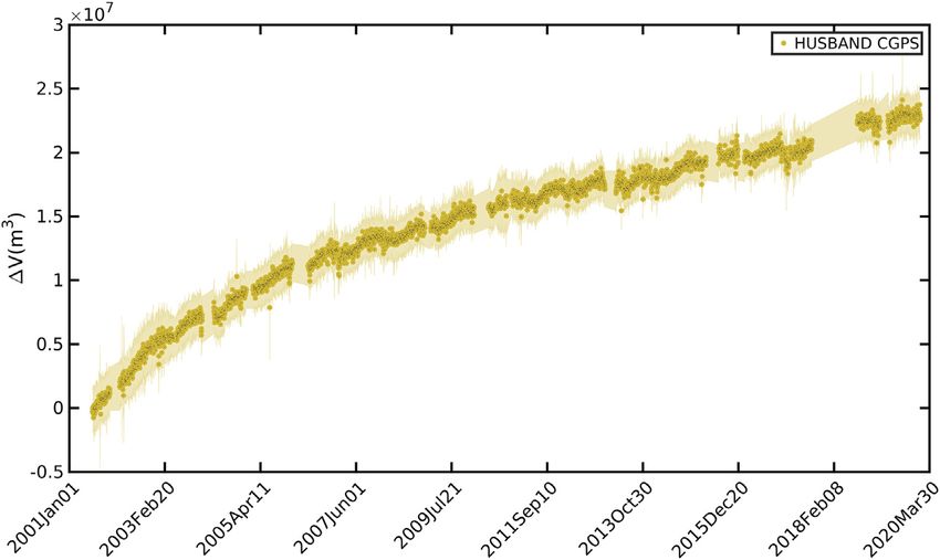
Rodríguez-Molina et al. Inter-Eruptive Volcano Uplift Time-Scales
the use of the “a priori” information from the data CΔV (and residual norm BV_ T2 − ΔV2. As recommended by Hansen
optional model, CV_ AT PA) covariance matrix. Such matrices (1992) we fit the log-log plot of discrete points with some
can be decomposed as: curves, choosing a 2D spline curve and then search for the
−1 truncation parameter by computing the L-corner (maximum
CΔV DDT curvature point). This corner of the spline curve is
−1 (5)
CV_ SST approximated to the closest discrete point. The L-corner is
located exactly where the solution changes in nature from
where the D (N × N) and S (M × M) matrices are determined
being dominated by regularization errors to being dominated
from the eigenvalue problem of each covariance matrix. In our
by the residual size. This regularization filters out the
case, no model covariance information is used, so CV_ I.CΔV is
estimator. The contribution of small singular values and noisy data.
obtained by error data propagation through ΔV
utility of D and S is the introduction of a transformed coordinate
system where data (and optional model) parameters each have
uncorrelated errors and unit variance. Therefore, ΔVnew DΔV, 5 RESULTS
V_ new SV_ and Bnew DBS−1 give the transformation of data,
model parameters and forward operator in the new system of 5.1 Re-Evaluation of Source Location and
coordinates. TSVD is applied to Bnew with a specific Geometry
regularization method to find the Principal Components of the We performed the Bayesian inversion for point source, prolate
observation set (ΔV). Then, the problem is back to the original spheroid and sill-like sources, with similar results. The results are
coordinates to achieve the solution and finally, the volume change represented in Figures 4, 5 and Tables 1, 2 report the prior
time-series is obtained by integrating the volume change rate in information and the PDFs with the 95% credible intervals for all
time: model parameters, respectively. The inversion reveals that the
surface displacements can be explained by a spherical point
_
V(t) Vδt (6) source with depth (4500–6000)m and ΔV (7–13)×106 m3, by a
sill-like source with depth (5600–7200)m, radius (220–400)m and
dimensionless excess pressure 0.05–0.30 and by a prolate
4.2.4 Regularization: Techniques Used for Truncation spheroid source with depth (5300–7400)m, major semi-axis
of Small Eigenvalues (240–720)m, aspect ratio (0.22–0.37)m, dimensionless excess
Some workable criteria for truncation in interdisciplinary pressure 0.38–8.61, strike angle (49–102)° and plunge (78–85)°.
problems include L-curve, Discrete Picard condition and The descending ERS Track 385 wrapped interferogram reveals a
Generalized cross validation (GCV) (Hansen, 1992; Hansen, near axisymmetric deformation pattern, with a maximum LOS
2007; Hansen and O’Leary, 1993). Methods like GCV surface displacement of ∼5 cm recorded at the center of the
sometimes fail to find the appropriate regularization parameter uplifting pattern (Figures 4A, D and G). Figures 4B, E and H
(flat local minima), whereas the L-curve gives a robust estimation present the predicted spherical point, sill-like and prolate
(Hansen and O’Leary, 1993) and the appropriate smoothing spheroid forward models, using the median value of the PDF
solution, which is very attractive from a mathematical point of of the model parameters. As expected from the deformation
view. We thus designed a strategy based on a L-curve to set up pattern, spherical point and sill-like models are very similar,
proper criteria to truncate the eigenvalues. suggesting that the geometry of the source is far from unique. The
First, we considered the Discrete Picard condition to explain extra modeling parameters of the prolate spheroid do not
the instability of the transformed linear inverse problem (Eq. 3) improve the misfit. Therefore, we favor the simplest spherical
and disregarded the smallest singular values (Hossainali et al., point source model over a sill-like and prolate spheroid source, to
2010; Hansen, 1990; Hansen, 2007): fit deformation pattern displayed in Figures 4A, D and G. Blue
T stars represent the horizontal location of spherical point, sill-like
V_ − V_ T ≤ P12 max ui ΔVi (7) and prolate spheroid estimated sources (Table 2). Figures 4C, F
1 2
1 ≤ i ≤ M−P si and I show the residuals between observed LOS displacement,
and spherical point, sill-like and prolate spheroid model
where V_ − V_ T1 2 is the regularization error, V_ and V_ T1 being the predicted displacements. The residual is larger close to the
exact and truncated SVD solutions; P is the regularization Three Sisters complex volcano (green triangles), due to orbital
parameter value, si are the singular values, and uTi ΔVi are and topographic contributions, and also in the western half of the
called Fourier coefficients (ΔVi are data and ui the uplift pattern, where data are less dense.
corresponding eigenvectors of the data space). The Discrete Figure 5 displays the histograms of marginal PDF for the four
Piccard condition is satisfied if, for all singular values larger spherical point, five sill-like and eight prolate spheroid source
than P, the corresponding Fourier coefficients decay faster on parameters. Black solid lines show the optimal values for the
average than si. corresponding model parameters. For the sill-like source, the
The L-curve method is applied to V_ T1 resulting in turn from radius and dimensionless excess pressure PDFs exhibit bi-
applying (Eq. 7) through a log-log plot of the norm of a modality (slightly unstable inversion result). For the prolate
regularized solution V_ T2 2 vs. the norm of the corresponding spheroid source, the aspect ratio between semi-axes and the
Frontiers in Earth Science | www.frontiersin.org 8 January 2021 | Volume 8 | Article 577588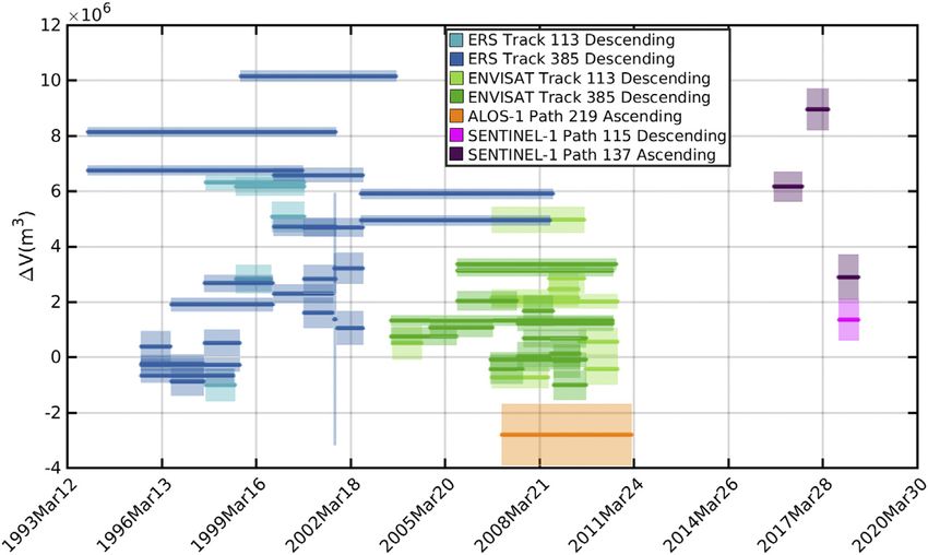
Rodríguez-Molina et al.                                                                                                           Inter-Eruptive Volcano Uplift Time-Scales

  FIGURE 5 | Posterior probability distributions for the Mogi, sill-like and prolate spheroid source models. Black solid lines show the optimal value for the
  corresponding model parameter (Tables 1, 2).

Frontiers in Earth Science | www.frontiersin.org                                     9                                           January 2021 | Volume 8 | Article 577588
Rodríguez-Molina et al.                                                                                                    Inter-Eruptive Volcano Uplift Time-Scales

  FIGURE 6 | Increments of volume change obtained for all interferograms (ERS, ENVISAT, ALOS-1 and SENTINEL-1), according with the median value for the
  source depth.

excess pressure PDFs display also a bi-modal shape. The major                      TABLE 1 | Prior information for the Elastic half-space Spherical Point Pressure
semi-axis PDF exhibits multi-modality.                                             (Mogi, 1958), Penny-shaped sill-like (Fialko et al., 2001) and Spheroid (Yang
                                                                                   et al., 1988) deformation sources.
5.2 Source Inflation Time-Series                                                                              Lower          Upper             Step          Start
We performed a CGPS and InSAR joint inversion to obtain the
time-line of volume changes, considering the best fitting source                    Mogi
                                                                                   Xcenter (m)            −1.00 × 10³     1.50   ×   104       25        2.00 × 10³
location for the point source geometry to better characterize the
                                                                                   Ycenter (m)            −1.00 × 10³     1.50   ×   104       25        2.00 × 10³
time-dependent inflation of the magma source at Three Sisters.                      Depth (m)                5 × 10²       2.00   ×   104       50        1.00 × 10³
   To apply our two-step-approach (section 3.2), we use the                        ΔV (×106 m3 )              0.1         1.00   ×   104   1.00 × 10⁻³       0.1
median, and 5% and 95% percentile values of the PDF of depth                       Sill
estimated by the Bayesian inversion. The corresponding values                      Xcenter (m)            −1.00 × 10³     1.50 × 10⁴           25        2.00 × 10³
                                                                                   Ycenter (m)            −1.00 × 10³     1.50 × 10⁴           25        2.00 × 10³
are: dmedian  5000 m, d5%  4500 m and d95%  6000 m. The
                                                                                   Depth (m)                5 × 10²       2.00 × 10⁴           50        1.00 × 10³
volume change time-series is determined using InSAR data from                      Radius (m)                 100            4,000             50           100
four satellite missions (ERS, ENVISAT, ALOS-1 and Sentinel-1),                     ΔP/μ                    1 × 10⁻⁵            10           1 × 10⁻⁶      1 × 10⁻²
on five different tracks and look angles, and CGPS data                             Spheroid
from HUSB.                                                                         Xcenter (m)            −1.00 × 10³     1.50 × 10⁴           25        2.00 × 10³
                                                                                   Ycenter (m)            −1.00 × 10³     1.50 × 10⁴           25        2.00 × 10³
   First, we obtain the increments of each volume change, ΔVi ,                    Depth (m)                5 × 10²       2.00 × 10⁴           50        1.00 × 10³
relating the Green’s functions (representing the source impulse                    Major semi axis (m)        100            4,000             50           100
for a buried point source) to the LOS deformation data observed                    Aspect ratio               0.2            0.99             0.01           0.5
along each satellite track and the three component CGPS data.                      ΔP/μ                    1 × 10⁻⁵            10           1 × 10⁻⁶      1 × 10⁻²
                                                                                   Strike (°)                  1              359               1           270
Figures 6, 7 respectively show results regarding estimation of the
                                                                                   Plunge (°)                  0               90               1            45
median value of source depth (dmedian  5000 m) for InSAR and
CGPS data. The cumulative increments of volume changes
detected at HUSB show gaps due to ice and snow
accumulation during winter. By means of the daily GPS                              Picard Plot provides no clues about the appropriate level of
measurements, the corresponding increments of volume                               truncation (Eq. 7). Therefore, we use L-curve to determine the
change, ΔVi , are more uniform for the CGPS data sets                              truncation level. L-curve criterion is fulfilled when L-corner
(Figure 7), but more variable for the individual SAR data sets                     1198, i.e., when only the first 24.1% nonzero singular values are
(Figure 6).                                                                        used in the inversion (Figure 8B).
   Finally, we applied the Picard Plot condition suitable to                          The analysis and results of the final inflation time-series are
understand the conditions of the ill-posed problem (Eq. 3).                        shown in Figures 9 and 10, and Tables 3 and 4. The inflation
Figure 8A shows    how   si only decays faster than the Fourier                time-series associated with the median estimation of the source
coefficients (uTi ΔVi ) for the smallest nonzero singular values.               depth suggests a maximum volume change rate of ∼ 1.60 ×
Hence, the problem can be considered stable, discarding the last                   106 m3 /yr during 1999–2001 and a subsequent rate as much as
10% of the singular values. Due to the stability of the problem, the               ∼ 0.75 × 10⁶ m3 /yr for the period 2015- January 2020. Data since

Frontiers in Earth Science | www.frontiersin.org                              10                                          January 2021 | Volume 8 | Article 577588
Rodríguez-Molina et al. Inter-Eruptive Volcano Uplift Time-Scales
TABLE 2 | Bayesian inversion results, with the median a posterior probability various source geometries such as spherical point, sill-like or
solution and the 95% credible intervals, for the Elastic half-space Spherical
crack and ellipsoidal. These different sources can all fit the data in
Point Pressure (Mogi, 1958), Penny-shaped sill-like (Fialko et al., 2001) and
Spheroid (Yang et al., 1988) deformation sources.
a satisfactory way. Our results are consistent with previous
findings (Table 3). However, volume change rates and depths
median 5% 95% vary slightly, possibly due to the fact that: 1) there may be a poorly
Mogi resolved deeper magma source, 2) inversions were limited to
Lon (°) −121.8382 −121.8418 −121.8350 purely kinematic models, 3) the source not being a stationary,
Lat (°) 44.1055 44.1030 44.1082 pressurized cavity in an isotropic elastic half-space, thus
Depth (m) 5,000 4,500 6,000 producing bias due to spatial or temporal considerations, 4)
ΔV (×106 m3 ) 8.99 6.98 12.66
Sill
diverse inversion techniques and related possible mathematical
Lon (°) −121.8368 −121.8398 −121.8339 artifacts, 5) different types of data sets and 6) ambiguity of source
Lat (°) 44.1018 44.0997 44.1041 geometries. We assumed a simple, stable, purely kinematic model
Depth (m) 6,300 5,600 7,200 as a valid approach, following the results of Dzurisin et al. (2009)
Radius (m) 250 220 400
and Riddick and Schmidt (2011), for estimating volume time
ΔP/μ 0.23 0.05 0.30
Spheroid
series. Now, we focus on discussing the implications of 3), 4), 5),
Lon (°) −121.8707 −121.8791 −121.8616 and 6).
Lat (°) 44.1187 44.1130 44.1228 We revisited the assumption of location stationarity of the
Depth (m) 6,100 5,300 7,400 inflation source, with focus on the most recent periods. Riddick
Major semi-axis (m) 400 240 720
and Schmidt (2011) already showed that the temporal evolution
Aspect ratio 0.28 0.22 0.37
ΔP/μ 1.85 0.38 8.61 of the uplift signal can be represented by a stationary volcanic
Strike (°) 68 49 102 source geometry and location with a decreasing inflation rate at
Plunge (°) 82 78 85 least from 1992 to 2010. The extent of deformation pattern
Geo-reference point is [−121.9, 44.03]°.
remains constant over 1992–2010 time period providing a
source depth range compatible with the uncertainties of
inversion models, as it is expected given that the extent of
2018 show a subtle, but significant change in the trend, instead of deformation pattern mainly depend on the source depth and
following asymptotic behavior. strength. The inversion for source parameters using Sentinel-1
interferograms (2014–2018) reveals very large uncertainties on
the parameters. Such results could be due to the interferograms’
6 DISCUSSION low signal-to-noise ratio caused by slower uplift rates during this
period. Nevertheless, the best fitting spherical sources are not able
6.1 Source Characterization to predict the observed displacements in the HUSB CGPS
Studies at Three Sisters using InSAR interferometric pairs and displacement time series. Moreover, the lack of substantial
stacks (Wicks, 2002; Riddick and Schmidt, 2011), GPS (campaign changes in the trends of each component of the HUSB CGPS
and continuous) and leveling (Dzurisin et al., 2009) assessed time series indicates that the source might not have changed
FIGURE 7 | Cumulative increments of volume changes for the CGPS station, Husband. The figure shows the results according with the median value for the
source depth.
Frontiers in Earth Science | www.frontiersin.org 11 January 2021 | Volume 8 | Article 577588Rodríguez-Molina et al. Inter-Eruptive Volcano Uplift Time-Scales
FIGURE 8 | (A) Discrete Picard Plot condition, suited for the analysis of ill-posed problems. The solution is stable when the Fourier coefficients, uTi ΔVi , on average
decay to zero faster than the reciprocal singular values, si. In this case, the problem can be consider stable, discarding the last 10% singular values. (B) L-curve showing
the trade-off between minimizing the residual norm (BV_ T2 − ΔV2 ) and minimizing the regularized solution size (V_ T2 ). The L-corner (represented in red) is located
2
exactly where the solution changes in nature from oversmoothing (i. e, dominated by regularization errors) to being dominated by residual size.
position. Therefore, we assumed the source has not changed period undergoing maximum deformation, displaying as much as
significantly either in shape nor in location since the onset of ∼5 cm of line-of-sight deformation (Figure 4). Selection of the
deformation. ERS-1 track 365 (descending orbit) interferometric pair spanning
A range of common techniques to estimate source location has August 1997- September 2000 satisfies both criteria. To reduce
been used, like forward modeling, grid search by iteratively fixing the signal-to-noise ratio, the interferogram is filtered for a pixel
of one parameter, arithmetic mean to obtain range values, or grid coherence threshold of 0.2. Other ERS-1 InSAR data were also
search. However, the Bayesian approach presents important processed for similar periods of time, but not used due to the low
advantages: 1) robust inversion for a single or more InSAR signal-to-noise ratio. No GPS data were available until 2001 and
interferograms with an acceptable signal-to noise-ratio and/or cannot be used to study the maximum uplift rate period.
GPS data, 2) rapid simultaneous inversion of all model We favor the simplest source, a spherical point source, to infer
parameters; 3) use of data uncertainty and prior model volume time series at Three Sisters. Our inversion results for
information; and 4) efficient sampling of posterior PDFs to spherical, prolate spheroid and a sill-like sources showed
estimate optimal model parameters and the associated range quantitatively similar results, in terms of data misfit and
of error. Bearing in mind such advantages, to obtain a robust surface displacement pattern. We noted that there is slightly
estimate of source geometry and location we only need geodetic elongated pattern of the InSAR data in the North-South direction
data with high spatial coverage, spanning the most appropriate (Figure 4). This pattern cannot be perfectly reproduced with an
period (shortest time, high deformation). For this, we use the axisymmetric source geometry. The elongation could be also be
Frontiers in Earth Science | www.frontiersin.org 12 January 2021 | Volume 8 | Article 577588Rodríguez-Molina et al. Inter-Eruptive Volcano Uplift Time-Scales
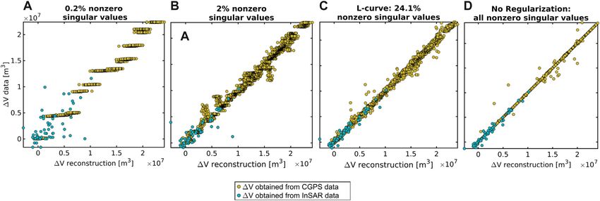
FIGURE 9 | ΔVi data (increment of volume change obtained from InSAR and CGPS deformation data, Eq. 1), vs. Simulated observations (ΔVireconstruction V(i+1) − Vi ,
Eq. 6). (A, B) Inversion solutions with regularization, using only the first 0.2 and 2% nonzero singular values, respectively (oversmoothing solution). (C) Regularized
solution using the L-curve criteria corresponding with 24.1% nonzero singular values (appropriate smoothing solution). (D) No regularization case (undersmoothing
solution).
TABLE 3 | Source location comparison for Three Sisters (assuming a Mogi source) from Previous Studies and the bayesian inversion carried out in this Study.
Inversion Depth (m) ΔV (106 m3 ) ΔVrate (106 m3 /yr)
1996–2000, InSARa 6500 ± 400 23.00 ± 3.00 ∼5.75 ± 0.75
2001–2008, Geodetic ground base datab 5,800 22.20 ∼3.14
1993–2008, InSARc 5200 ± 100 57.00 [+1.95, −3.60] ∼3.80 [+0.13, −0.24]
1997–2000, InSAR [this study]d 5000 [+1000, −500] 8.99 [+3.67, −2.01] ∼3.00 [+1.22, −0.67]
a
ERS Descending (08/1996–10/2000) (Wicks, 2002).
b
Campaign GPS, CGPS and Leveling (05/2001-late 2008) (Dzurisin et al., 2009).
c
ERS Track 385 Descending (08/1993-08/2008) (Riddick and Schmidt, 2011).
d
ERS Track 385 Descending (08/1997-09/2000).
caused by the topography of Three Sisters area at the east side of reasonable to assume the spherical point source as the simplest
the deforming area or tropospheric delays in the interferometric kinematic model that explains the signal. Furthermore, the values
data. To robustly distinguish between different source geometries, for depth and increments of volume change lie within our 95%
we must have full three dimensional surface displacements credible intervals (Table 3). Wicks (2002) processed three
(Dieterich and Decker, 1975). Therefore, in our case, the interferograms, obtaining an increment of volume change of
almost symmetric shape of the 2D deformation pattern ΔV 23 × 106 m3 and depth of 6500 m for the one with the
implies that source geometry remained far from being largest apparent signal-to-noise ratio. Ultimately, a deeper source
uniquely resolved. Nevertheless, to accept more complex will trade-off with a greater ΔV, to fit the same surface
geometries than spherical, we should have obtained deformation. Although the time acquisition of the best
significantly lower data misfit values. Furthermore, the interferogram of Wicks (2002) spans only 1 year more than
spheroid modeling residuals are not fully consistent with the our InSAR data interferometric pair, the important difference
observed pattern in the western area of deformation (Figures 4I). between our ΔVrate ∼ 3.00 × 10⁶ m3 /yr and their ΔVrate
In this case, we also consider that the topography could have a ∼ 5.75 × 10⁶ m3 /yr is mainly due to their depth estimation.
minor effect because the highest topographic relief is Our InSAR interferogram matches one of the other two by
concentrated on the far field area of deformation signal. Wicks (2002). For that interferogram, their model gives depths
Therefore, we assume that the noted asymmetry in the InSAR ∼1 km shallower, being closer to our depth estimation.
data should not affect the overall interpretation of the time series
of volume changes.
The differences between inversion methods and data selection 6.2 Time Series of Volume Changes:
might explain that our optimal inversion results suggest a slightly Regularization Using the Truncated SVD
shallower source with a corresponding smaller increment of To assess the effect of the regularization, we compared the
volume change. Despite that, considering that the models fit increments of volume change (ΔVi , Eq. 1) and the
the data well and yield similar misfit values, we conclude that it is corresponding simulated observations ( ΔVireconstruction
Frontiers in Earth Science | www.frontiersin.org 13 January 2021 | Volume 8 | Article 577588Rodríguez-Molina et al. Inter-Eruptive Volcano Uplift Time-Scales
FIGURE 10 | Volume change time series for a Mogi source (constrained by both the GPS and InSAR data), at different depth estimations (Table 1): median value
(light green), 95 and 5% percentile values (yellow and dark green). Cian solid lines represent predicted curves through Non Linear Least Squares (NLS), Least Absolute
Residuals (LAR) method, following the e-folding characteristic shape function of Eq. 8. Stars show the location of the beginning of the exponential function: for data
associated with median depth value estimation (light green), 95 and 5% percentile values (yellow and dark green).
TABLE 4 | e-folding parameters obtained by NonLinear Least Squares, using the 6.3 Time-Scales of Inter-Eruptive Uplift
Least Absolute Residual method (LAR). Signals: Three Sisters and Other Volcanoes
Value c (yr−1) 1/c(yr) t0 (yr) R–square RMSE The continuous and extended regularized time-series of volume
change allows us to study the inflation process in detail. Riddick and
Optimal 0.1055 9.48 1999.09 0.989 0.60 × 10⁶ Schmidt (2011) proposed a piece-wise linear parametrization with
Lower bound 0.1042 9.60 1998.75 0.998 0.18 × 10⁶
two changes in rate provides a good fit to uplift rates till 2009
Upper bound 0.1074 9.31 1999.59 0.988 0.87 × 10⁶
explaining two different inflation processes beginning at 1998 and
Upper and lower bounds for the curve fitting parameters, encompassing the results for 2004 at Three Sisters. This model was supported by the detection of a
the volume changes series related to the 5%, median and 95% percentile values of
source depth estimate.
seismic swarm in 2004. Our denser, longer time-series clearly shows
a smooth and continuous function, which we interpret as a fast
V(i+1)inversion − Viinversion from the results of Eq. 6) for different inflation followed by relaxation of the crust (Figure 10). We are
levels of regularization. Figures 9A, B show the solution for specifically interested on the interval of decaying rates.
an extreme regularization, using only the first 0.2% and 2% Consequently, the time-series is divided into two main
nonzero singular values (oversmoothing solutions). For the intervals separating increasing and decaying behavior of
0.2% case, the values of ΔVi associated with the InSAR data volume rates. An exponential function can reasonably
display a wide dispersion, and the ΔVi associated with GPS reproduce the relaxation process. Therefore, we propose a
data acquire discrete values, i.e., the same ΔVi value is piece-wise parametric of the form:
obtained for many different time intervals. Figure 9D
represents the case of non-regularization (less filtering, d, t < t0
V(t) (8)
maximum solution size and minimum misfit). The residual a − bexp − (c · (t − t0 )), t ≥ t0
in Figure 9D is minimized because the solution reproduces
even the seasonal perturbations of the GPS data where a, b and d are constants, 1/c ϵ is the characteristic relaxation
(undersmoothing solution). There is a seasonal time constant, here after named e-folding parameter, and t0 is the
deformation of the crust associated with the surface load start of the exponential trend. We solved the parameters of this
of the snow cover. It is possible that the magma reservoir’s model using a non-linear least-square fit. To minimize the influence
internal pressure also fluctuates seasonally in response to this of outliers, we used regression method: the Least Absolute Residuals
effect. However, from CGPS data alone we cannot resolve the (LAR) and Bisquare weights methods, considering also the data
cause of these fluctuations. Therefore, a smoother solution is uncertainties (weighted). Four methods (Bisquare, Bisquare-
preferred to depict the long-term deformation time series. Weighted, LAR, LAR-Weighted) show very similar fit, LAR
This is given by the combination of Picard condition and performing the best (Figure 10; Table 4). Time-series from the
L-curve criteria; it corresponds to the appropriate smoothing median, and 5% and 95% percentiles of the PDF distribution for
solution, i.e, 24.1% nonzero singular values (Figure 9C). depth, along with the variance of the curve fitting, permit
Frontiers in Earth Science | www.frontiersin.org 14 January 2021 | Volume 8 | Article 577588You can also read