Satellite observations of aerosols and clouds over southern China from 2006 to 2015: analysis of changes and possible interaction mechanisms ...
←
→
Page content transcription
If your browser does not render page correctly, please read the page content below
Atmos. Chem. Phys., 20, 457–474, 2020
https://doi.org/10.5194/acp-20-457-2020
© Author(s) 2020. This work is distributed under
the Creative Commons Attribution 4.0 License.

Satellite observations of aerosols and clouds over southern
China from 2006 to 2015: analysis of changes and possible
interaction mechanisms
Nikos Benas1 , Jan Fokke Meirink1 , Karl-Göran Karlsson2 , Martin Stengel3 , and Piet Stammes1
1 R&D  Satellite Observations, Royal Netherlands Meteorological Institute (KNMI), De Bilt, the Netherlands
2 Swedish Meteorological and Hydrological Institute (SMHI), Norrköping, Sweden
3 Deutscher Wetterdienst (DWD), Offenbach, Germany

Correspondence: Nikos Benas (benas@knmi.nl)

Received: 14 September 2018 – Discussion started: 4 October 2018
Revised: 9 October 2019 – Accepted: 29 November 2019 – Published: 14 January 2020

Abstract. Aerosol and cloud properties over southern China       1   Introduction
during the 10-year period 2006–2015 are analysed based on
observations from passive and active satellite sensors and       The role of atmospheric aerosols in climate change has been
emission data. The results show a strong decrease in aerosol     studied widely in the past. Their various effects are broadly
optical depth (AOD) over the study area, accompanied by an       defined based on their interactions with atmospheric radia-
increase in liquid cloud cover and cloud liquid water path       tion and clouds. The direct effect is described through the
(LWP). The most significant changes occurred mainly in late      scattering and absorption of radiation, whereas indirect ef-
autumn and early winter: AOD decreased by about 35 %, co-        fects describe interactions with clouds, which can lead to
inciding with an increase in liquid cloud fraction by 40 % and   changes in both cloud albedo (Twomey, 1977) and cloud
a near doubling of LWP in November and December. Anal-           lifetime (Albrecht, 1989). The semi-direct effect is a third
ysis of emissions suggests that decreases in carbonaceous        category that describes aerosol-induced changes in clouds
aerosol emissions from biomass burning activities were re-       through interaction with radiation. According to the latest
sponsible for part of the AOD decrease, while inventories        terminology (Boucher et al., 2013), the semi-direct effect is
of other, anthropogenic emissions mainly showed increases.       described as a “rapid adjustment” induced by aerosol radia-
Analysis of precipitation changes suggests that an increase      tive effects, and along with the direct effect it is grouped
in precipitation also contributed to the overall aerosol re-     into the “aerosol–radiation interactions” (ARIs) category,
duction. Possible explanatory mechanisms for these changes       whereas the indirect effects are termed “aerosol–cloud inter-
were examined, including changes in circulation patterns         actions” (ACIs).
and aerosol–cloud interactions (ACIs). Further analysis of          Observations of these mechanisms and their effects on
changes in aerosol vertical profiles demonstrates a consis-      climate have been elusive, and the uncertainties associated
tency of the observed aerosol and cloud changes with the         with them remain high (Boucher et al., 2013). The main
aerosol semi-direct effect, which depends on relative heights    reasons for this lack of substantial progress originate in the
of the aerosol and cloud layers: fewer absorbing aerosols in     high complexity of these phenomena, with multiple possible
the cloud layer would lead to an overall decrease in the evap-   feedback mechanisms and dependences on various parame-
oration of cloud droplets, thus increasing cloud LWP and         ters in different regimes (Stevens and Feingold, 2009; Bony
cover. While this mechanism cannot be proven based on the        et al., 2015). Although there are continuous improvements,
present observation-based analysis, these are indeed the signs   the mechanisms related to aerosol and cloud interactions and
of the reported changes.                                         feedbacks are still inadequately represented in models (Fein-
                                                                 gold et al., 2016) and poorly captured by remote sensing
                                                                 measurements (Seinfeld et al., 2016). Regarding the latter

Published by Copernicus Publications on behalf of the European Geosciences Union.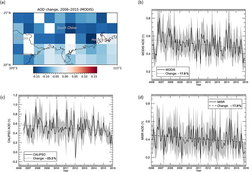
458                  N. Benas et al.: Satellite observations of aerosols and clouds over southern China from 2006 to 2015

approach, many studies have highlighted the difficulties and      (CALIPSO) data. MODIS is a sensor on board NASA’s Terra
limitations of remote sensing methods, which usually include      and Aqua polar orbiters, providing aerosol and cloud data
limitations in spatial and temporal samplings (Grandey and        products since 2000 and 2002 from Terra and Aqua respec-
Stier, 2010; McComiskey and Feingold, 2012). On the other         tively. The Aqua MODIS level 3 collection 6 daily aerosol
hand, progress is steadily being made, as data sets of aerosols   optical depth (AOD) was used here, available over both land
and clouds based on remote sensing retrievals gradually im-       and ocean at 1◦ × 1◦ spatial resolution (Levy et al., 2013).
prove. Additionally, independent data sets with complemen-           AOD data from MISR were also analysed. MISR flies
tary characteristics and properties become constantly avail-      on board NASA’s Terra satellite and acquires measurements
able, allowing for more in-depth analyses of the aerosol and      at nine viewing angles, providing information on specific
cloud conditions and opening new possibilities for combined       aerosol types along with the total aerosol load (Khan and
usage, including further constraining the effects of aerosols     Gaitley, 2015). Here, MISR products of total AOD, along
on clouds.                                                        with fine-mode, coarse-mode and (non-spherical) dust par-
   The present study builds on these developments by pro-         ticle AOD were analysed on a monthly basis and at 1◦ × 1◦
viding an analysis of aerosol and cloud characteristics and       spatial resolution, available at level 3 of version 23.
changes in recent years over a climatically important and            The CALIPSO level 3 monthly aerosol profile product was
sensitive area in southern China. This region (20–25◦ N,          also used to include information on the aerosol vertical dis-
105–115◦ E) was selected, as it is a densely populated area       tribution in the analysis. CALIPSO level 3 parameters are
with intense human activities, ranging from urban and in-         derived from the corresponding instantaneous level 2 ver-
dustrial to agricultural areas, which also constitute differ-     sion 3 aerosol product (Winker et al., 2009; Omar et al.,
ent sources of aerosol emissions. Furthermore, significant        2009; Tackett et al., 2018) and include column AOD of to-
changes in aerosol loads during the past years over the wider     tal aerosol, available globally at 2◦ × 5◦ latitude/longitude
surroundings have previously been reported (e.g. Zhao et al.,     resolution, along with the extinction profiles at 60 m vertical
2017; Sogacheva et al., 2018), providing the opportunity for      resolution, up to 12 km altitude. The standard quality filters
an analysis of possible effects on clouds. Hence, the pur-        implemented to ensure the quality of the level 3 product, de-
pose of this study is twofold. The primary aim is to anal-        scribed in Tackett et al. (2018), were also adopted here.
yse aerosol and cloud characteristics and changes during the         Apart from the analysis of aerosol loads and vertical distri-
period 2006–2015 over southern China. Using multiple data         butions over the region with MODIS, MISR and CALIPSO
sets, created based on different retrieval approaches, adds ro-   data, aerosol sources were investigated using the Global
bustness to the results. The secondary purpose of this study      Fire Emissions Database (GFED) and the Copernicus Atmo-
is to investigate the possibilities and limitations of the com-   sphere Monitoring Service (CAMS) emissions inventories.
bined use of this multitude of aerosol and cloud data sets for    GFED provides information on trace gas and aerosol emis-
the assessment of possible explanatory mechanisms, includ-        sions from fires on a global scale. Here, organic carbon (OC)
ing large-scale changes and local-scale aerosol and cloud in-     and black carbon (BC) data were analysed, based on the lat-
teractions. For this purpose, data sets are analysed in combi-    est version 4 of the data set (GFED4s). They are available
nation to either help exclude possible explanations or provide    at 0.25◦ × 0.25◦ spatial resolution and on a monthly basis.
indications of their manifestation.                               GFED emission estimates are based on data of burned areas
   The study is structured as follows: Sect. 2 provides a de-     and active fires, land cover characteristics and plant produc-
scription of the aerosol, emissions and cloud data sets used      tivity, and the use of a global biogeochemical model (Van der
and the methodology for analysing their changes. Results          Werf et al., 2017). The CAMS global anthropogenic emis-
of this analysis include time series and seasonal changes in      sions inventory provides emission information for a multi-
aerosols and clouds, presented in Sect. 3, and possible effects   tude of species and sources, including transport, industry,
of large-scale meteorological variability and indications of      power generation, waste handling and agriculture, also on a
possible effects of aerosol changes on corresponding cloud        monthly basis and at 0.1◦ ×0.1◦ (Granier et al., 2019) resolu-
changes, described in Sect. 4. Our findings are summarized        tion. It should be noted that, due to the long-range transport
in Sect. 5.                                                       of aerosols, local aerosol emissions will not always fully ex-
                                                                  plain corresponding properties and characteristics of aerosol
                                                                  types and loads in the atmosphere of the same region. The
2     Data and methodology                                        adequacy of local emissions in this role will depend on the
                                                                  effect that long-range transport may have, either removing
2.1    Aerosol, emissions and precipitation data                  aerosols from the region or adding more loads from adjacent
                                                                  regions. To assess the magnitude of these effects in the study
Analysis of aerosol changes was based on Moderate                 region, an air mass trajectory analysis was also performed to
Resolution Imaging Spectroradiometer (MODIS), Multi-              supplement local emissions.
angle Imaging SpectroRadiometer (MISR), and Cloud-                   While emission data records provide a useful source of
Aerosol Lidar and Infrared Pathfinder Satellite Observations      possible aerosol sources, decreases in aerosol loads can also

Atmos. Chem. Phys., 20, 457–474, 2020                                               www.atmos-chem-phys.net/20/457/2020/
N. Benas et al.: Satellite observations of aerosols and clouds over southern China from 2006 to 2015                           459

originate in other phenomena, e.g. an increase in precipita-       contributions from systematic and random errors. Similarly,
tion apart from decreasing emissions. Hence, to achieve a          validation at monthly scales is cumbersome, and no valida-
more complete overview of the possible reasons that led to         tion results for level 3 have been reported for the data sets
the aerosol changes reported here, rainfall data were also         used in this study.
analysed. For this purpose, the Global Precipitation Clima-           Therefore, the use of three independent aerosol data sets
tology Project (GPCP) version 2.3 data record was used             and two cloud data sets, derived from different sensors is
(Adler et al., 2018). The GPCP monthly product integrates          an important element of this study, which suggests that the
precipitation estimations from various satellites over land        detected changes reflect actual changes rather than possible
and ocean with gauge measurements over land at a 2.5◦ ×            sensor degradations or retrieval artefacts. This is especially
2.5◦ resolution.                                                   true in the case of aerosol data, which were obtained by dif-
                                                                   ferent retrieval approaches.
2.2   Cloud data
                                                                   2.4   Analysis of time series and changes
Two independently derived, satellite-based cloud data sets
were used for the analysis of cloud properties and changes         The analysis of all data sets and their changes was based on
over southern China. The Aqua MODIS level 3 collection 6           monthly average values. This temporal resolution is appro-
daily 1◦ ×1◦ product was used (Platnick et al., 2017), as in the   priate for studying both long-term interannual as well as sea-
case of AOD, for the estimation of monthly averages and cor-       sonal changes. Furthermore, data from afternoon satellites
responding changes in cloud properties, including total and        were mainly used (MODIS Aqua, AVHRR on NOAA-18 and
liquid cloud fractional coverage (CFC), in-cloud and all-sky       NOAA-19, and the daytime product of CALIPSO) to mini-
liquid water path (LWP), as well as liquid cloud optical thick-    mize differences due to different temporal samplings. Addi-
ness (COT) and effective radius (REFF).                            tionally, due to the different grid cell sizes of the products
   The same cloud properties were analysed using the sec-          used, the analysis was based only on area-weighted averaged
ond edition of the Satellite Application Facility on Climate       values over the entire study region rather than individual grid
Monitoring (CM SAF) cLoud, Albedo and surface RAdiation            cells. Area-weighted averages were computed based on the
dataset from AVHRR (Advanced Very High Resolution Ra-              cosines of the latitudes of the grid cells covering the study
diometer) data (CLARA-A2), a recently released cloud prop-         region. However, due to the small size of the domain the
erty data record, created based on AVHRR measurements              ensuing differences were minor. It should be noted that, in
from NOAA and MetOp (Meteorological Operational Satel-             the case of the two emission data sets GFED and CAMS,
lite Program of Europe) satellites (Karlsson et al., 2017). It     monthly values of emissions over the study area were cal-
covers the period from 1982 to 2015 and includes, among            culated by summing the corresponding grid cell values, in-
other parameters, CFC and cloud phase (liquid or ice), and         stead of averaging. Additionally, in the case of CALIPSO,
cloud top properties and cloud optical properties, namely          spatial averages were weighted by the number of samples
COT, REFF and water path, separately for liquid and ice            used, which is available in the level 3 data.
clouds. Orbital drift in NOAA satellites is an important is-          The quantification of changes during the study period was
sue regarding the stability of the CLARA-A2 time series,           based on linear regression fits to the spatially averaged desea-
especially in the 1980s and 1990s. For the 10-year period          sonalized monthly time series. Deseasonalization was per-
examined in this study, CLARA-A2 level 3 data, available at        formed by subtracting from each month the corresponding
0.25◦ × 0.25◦ spatial resolution from AVHRR on NOAA-18             time series average of this month and then adding the average
and NOAA-19 were used. Specifically, only the “primary”            of all months in the time series. For every variable X studied,
satellite was used in each month, meaning that when NOAA-          the change 1X was calculated as 1X = Xf − Xi , where Xi
19 data became available, NOAA-18 was not used anymore.            and Xf are the initial and final monthly values of the regres-
As a result, orbital drifts are minor.                             sion line. The corresponding percent change was estimated
                                                                   as 1X = 100(Xf − Xi )/Xi .
2.3   Uncertainties in aerosol and cloud products                     Spatial and temporal representativeness of the study area
                                                                   and time period in the change analysis were ensured by ap-
Uncertainties in pixel-based (level 2) data can in many cases      plying thresholds to both the area covered with valid data and
be estimated by propagation of error sources through the           the number of months used in the calculations. Specifically,
retrieval algorithms and through validation with co-located        the following thresholds were applied:
independent reference observations. For example, Levy et
al. (2013) showed by comparison with Aerosol Robotic Net-            a. On a grid cell basis, a monthly average value was used
work (AERONET) observations that the MODIS AOD has                      only if it was computed from at least 18 daily values
a 1σ uncertainty of about ±(0.05 + 0.15AOD) over land.                  (10 daily values for AOD, due to sparsity of data). Ap-
However, the propagation of pixel-based error estimates to              plication of this threshold requires the number of days
monthly aggregates is difficult because it needs to separate            used in the calculation of the monthly average. This in-

www.atmos-chem-phys.net/20/457/2020/                                                   Atmos. Chem. Phys., 20, 457–474, 2020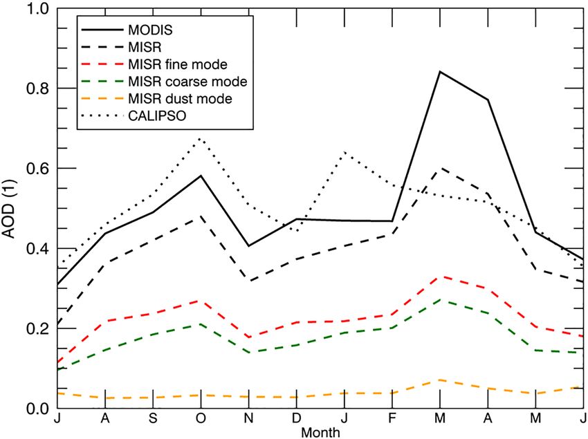
460 N. Benas et al.: Satellite observations of aerosols and clouds over southern China from 2006 to 2015
formation was available in all data sets used, except for
MISR.
b. A spatially averaged value was used if it was computed
from at least 50 % of the grid cells in the study area.
c. It was required that at least 80 % of monthly averages
are present in the time series, for the corresponding 10-
year changes to be estimated.
Further analysis included an estimation of changes per
month, in order to assess their seasonal variation. In this case,
no deseasonalization was applied. Statistical significance of
all calculated changes was estimated using the two-sided t
test, with a confidence interval of 95 %.
3 Results Figure 1. Seasonal variation in aerosol optical depth over southern
China, based on the period 2006–2015, from MODIS, MISR and
3.1 Aerosol and emissions characteristics and changes CALIPSO, including MISR fine- and coarse-mode and dust particle
AOD. Note that the horizontal axis starts in July and ends in June.
Figure 1 shows the seasonal variation of AOD from MODIS,
MISR and CALIPSO over southern China, based on data dur-
ing 2006–2015. MODIS, MISR and CALIPSO total AOD total AOD during the 10-year period is apparent and statis-
are in relatively good agreement in most months, with the tically significant in the 95 % confidence interval in all three
largest differences occurring in March and April, when time series and covers large parts of the study region (see
CALIPSO deviates from the other two data sets. While the also Figs. S1 and S2 in the Supplement; additional informa-
present analysis was designed to minimize discrepancies due tion on the time series analysis, i.e. slopes and p values, is
to differences in spatial and temporal resolutions, as de- given in Table S1). The reduction in AOD reported here is in
scribed in Sect. 2.3, some disagreement between CALIPSO agreement with changes over the same region or wider Chi-
and the passive sensors should be expected, considering their nese regions during recent years, reported based on different
differences in areas sampled, overpass times and retrieval satellite sensors, e.g. MODIS (He et al., 2016), MODIS and
methodologies. While it was not possible to pinpoint spe- AATSR (Advanced Along-Track Scanning Radiometer) (So-
cific reasons for the March–April differences based on the gacheva et al., 2018), and MODIS and MISR (Zhao et al.,
data sets used here, this feature deserves further investiga- 2017).
tion. Based on MISR, which offers additional information on The seasonal variability of aerosols over the study region
aerosol types, the fine-mode and coarse-mode AODs, which (Fig. 1) suggests that their changes could also exhibit sea-
add up to the total AOD, follow a seasonal pattern similar to sonal variations. Hence, the time series changes in AOD were
the latter. The fine-mode AOD, which constitutes a large part further analysed in terms of their seasonal variability. Results
of the total, highlights the important role that anthropogenic are shown in Fig. 3. It is apparent that the main decrease oc-
emissions play in the overall aerosol load over the region. curs in autumn and early winter. All three data sets agree
On the other hand, the contribution of dust is minimal, with a well in this seasonal pattern. Based on MISR, this decrease
small peak in spring. This is probably due to the long distance is driven primarily by fine-mode and secondarily by coarse-
of the study region from deserts, which constitute major dust mode aerosols, as reported earlier, while dust aerosols show
sources. no significant change.
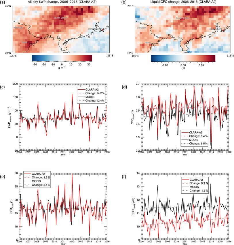
Figure 2 shows the changes in AOD over the southern The same analyses of seasonal variability and changes
China region during the 10-year period examined, both on were also performed for emission sources in the region,
a grid cell basis from MODIS (Fig. 2a) and as spatially which could possibly explain part of the AOD characteris-
averaged time series from MODIS, CALIPSO and MISR tics. These include local fire emissions of organic carbon
(Fig. 2b, c and d). The grid-cell-based changes in AOD (OC) and black carbon (BC) particles from GFED, as well
(Fig. 2a) reveal an almost uniform reduction throughout the as anthropogenic emissions of OC, BC, SO2 , NOx and NH3
area, with stronger decreases over land. The time series from CAMS, the latter three acting as sulfate and nitrate
of the deseasonalized spatially averaged monthly values of aerosol precursor gases. Figure 4a shows that GFED emis-
the AOD, separate from MODIS, CALIPSO and MISR, are sions exhibit a strong seasonality, with the highest occurring
shown in Fig. 2b, c and d, along with their linear regression between November and April. The emissions from CAMS
fits and corresponding changes (in percent). The reduction in exhibit almost no seasonal variation (Fig. S3), since there is
Atmos. Chem. Phys., 20, 457–474, 2020 www.atmos-chem-phys.net/20/457/2020/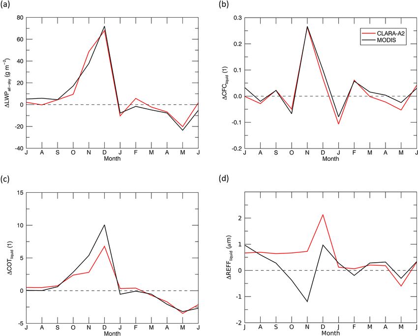
N. Benas et al.: Satellite observations of aerosols and clouds over southern China from 2006 to 2015                                  461

Figure 2. Changes in AOD over southern China from 2006 to 2015. (a) Spatial distribution of AOD change over the study region deduced
from MODIS data. Spatially averaged monthly deseasonalized values of AOD from MODIS (b), CALIPSO (c) and MISR (d). Shaded areas
correspond to one standard deviation of the grid-scale monthly averages. Dotted lines correspond to linear regression fits. Percent changes
during the period examined are also shown, with the statistically significant ones indicated in bold.

                                                                        no strong seasonality in the activities producing them, e.g.
                                                                        industrial emissions and transportation. On the other hand,
                                                                        biomass burning seasonality might be explained by activi-
                                                                        ties which exhibit seasonal variation, such as crop residue
                                                                        burning, firewood consumption and agricultural-waste open
                                                                        burning (Chen et al., 2017). It should be noted, however, that
                                                                        the GFED emissions are limited to open fire events, and thus
                                                                        they should not be regarded as representative of all biomass
                                                                        burning activities in the region.
                                                                           Analysis of changes in OC and BC emissions from GFED
                                                                        shows an overall decrease in emitted particles, with the
                                                                        largest occurring from late autumn to early spring (Fig. 4b),
                                                                        with a minimum in November. Analysis of other major an-
                                                                        thropogenic emission sources in the region reveals increases
                                                                        during the period examined (Fig. 5). While these results may
                                                                        at first seem contradictory to the general consensus on the
Figure 3. Seasonal variation of changes in AOD over south-              reduction of anthropogenic emissions in China during recent
ern China from 2006 to 2015 deduced from MODIS, MISR and                years (see e.g. Van der A et al., 2017), it should be noted that
CALIPSO data. MISR data include fine- and coarse-mode and dust
                                                                        emission patterns are not uniform throughout China. Instead,
particle AOD.

www.atmos-chem-phys.net/20/457/2020/                                                         Atmos. Chem. Phys., 20, 457–474, 2020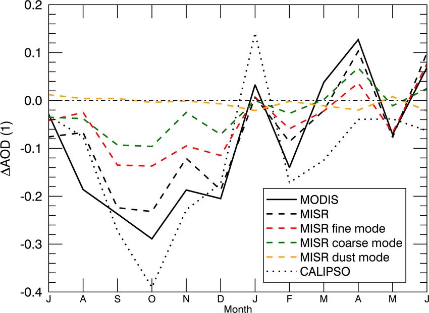
462                   N. Benas et al.: Satellite observations of aerosols and clouds over southern China from 2006 to 2015

                                                                     Figure 5. Emissions of aerosols and precursor gases from the
                                                                     Copernicus Atmosphere Monitoring Service. The emissions have
                                                                     been aggregated to annual totals over the southern China study area
                                                                     and plotted relative to the year 2006.

                                                                     examined: precipitation and long-range transport. As men-
                                                                     tioned in Sect. 2.1, changes in precipitation are also a fac-
                                                                     tor that can lead to changes in aerosol concentrations. For
                                                                     this reason, a similar analysis of GPCP precipitation data
                                                                     was performed, with the results shown in Fig. 6. The sea-
                                                                     sonality pattern (Fig. 6a) shows higher precipitation values
                                                                     appearing in summer months, compared to winter. Precipi-
Figure 4. (a) Seasonal variation in organic and black carbon emis-   tation has overall increased by 11.2 % over the region dur-
sions from GFED (in Gg C) over southern China from 2006 to 2015.
                                                                     ing the study period (Fig. 6b), although not in a statistically
(b) Corresponding changes on a monthly basis (in Gg C per month)
                                                                     significant sense. It should be noted, however, that increased
during the same period.
                                                                     precipitation in southern China during the same period is also
                                                                     reported elsewhere (see e.g. Fig. 3b in Zhang et al., 2019).
                                                                     Examination of monthly changes shows that this increase
differences should be expected on the provincial level, such         appeared mainly in autumn and early winter (September–
as in this study. Furthermore, large-scale implementations of        December), largely coinciding with the decrease in aerosols
emission policies in China in specific past years render simi-       (Fig. 3), while a significant precipitation decrease occurred in
lar analysis very sensitive to the time range selected.              June. Further correlation analysis showed that precipitation
   A direct comparison of changes in AOD and GFED sur-               changes anti-correlate significantly with AOD changes from
face emissions, which are both satellite based, offers addi-         MODIS and MISR in September–December (see Sect. 3.3).
tional insights into the origins of these changes: in cases          These results suggest that wet removal played a role in the
where AOD and emissions changes agree well, such as in               decrease in AOD reported for the same period.
November and December, when both AOD and biomass                        A long-range transport analysis was also performed, since
burning decrease (Figs. 3 and 4b), it can be hypothesized that       a change in AOD could also be caused by the transporta-
the former played a role in the latter. While this cause-and-        tion of adjacent air masses to or from the study region. For
effect mechanism cannot be proved based on observations              this purpose, forward- and back-trajectory analyses were per-
only, this hypothesis can be further supported by examin-            formed using the Hybrid Single-Particle Lagrangian Inte-
ing correlations between the two data sets (this is done in          grated Trajectory (HYSPLIT) model. HYSPLIT is a pub-
Sect. 3.3). In cases where there is an obvious disagreement          lic domain model (https://ready.arl.noaa.gov/HYSPLIT.php,
between emissions and AOD changes (e.g. in September and             last access: 20 December 2019), suitable for analysing air
October), additional reasons for the AOD reduction must be           mass trajectories (Draxler and Hess, 1998). For the present
sought.                                                              study, the analysis setup was as follows: October and Novem-
   Two additional mechanisms that could explain the de-              ber were selected to be analysed in terms of long-range trans-
crease in AOD in the absence of decreasing emissions were            port. October is the month with the largest discrepancies

Atmos. Chem. Phys., 20, 457–474, 2020                                                   www.atmos-chem-phys.net/20/457/2020/
N. Benas et al.: Satellite observations of aerosols and clouds over southern China from 2006 to 2015 463 Figure 6. (a) Seasonal variation of precipitation in the southern China study region based on Global Precipitation Climatology Project data. (b) Corresponding spatially averaged monthly deseasonalized values. The dotted line corresponds to the linear regression fit. (c) Seasonal variation of changes in GPCP precipitation. Seasonal averages and changes in panels (a) and (c) are based on data from the period 2006 to 2015. www.atmos-chem-phys.net/20/457/2020/ Atmos. Chem. Phys., 20, 457–474, 2020
464                  N. Benas et al.: Satellite observations of aerosols and clouds over southern China from 2006 to 2015

between changes in AOD (large decrease, see Fig. 3) and                Figure 8 shows grid cell based and spatially averaged
local emissions (practically no change, see Fig. 4b), while         changes in cloud properties over southern China during the
in November large changes are reported in AOD (Fig. 3),             period examined. The all-sky LWP and liquid CFC have in-
biomass burning emissions (Fig. 4b) and clouds (discussed           creased over most parts of the land and significantly in most
later in Sect. 3.2). For October and November 2007 and              cases (Fig. 8a and b, with corresponding maps of statistical
2015, representing conditions close to the beginning and end        significance levels given in Fig. S8). In fact, Fig. 8 shows
of the study period respectively, HYSPLIT was run for tra-          increases in all liquid cloud properties, with the largest in-
jectories starting every 6 h and lasting 24 h each, during the      crease found for the total liquid water content present in
whole month, at two heights, 500 and 1500 m above sea level.        clouds (12 %–14 %). Liquid COT variations appear similar
Both forward and back trajectories were analysed, starting          to those of LWP, with very good agreement between the two
and ending at the centre of the study region. The forward-          data sets (CLARA-A2 and MODIS). COT changes are pos-
trajectory analysis was performed to give insights into the         itive, while liquid REFF changes are also positive but more
degree of dispersion of locally emitted aerosol loads outside       ambiguous. Cloud changes appear statistically significant at
of the study region, while the back-trajectory analysis reveals     the 95 % level over large areas of the study region, especially
how frequently the air masses found in the study region orig-       over land, when studied on a grid cell basis. Analysis of spa-
inate outside of it.                                                tially averaged values, however, over the entire (5◦ × 10◦ )
   The results, shown in Figs. S4 and S5 for the October for-       study region, reduces this significance to levels below 95 %
ward and back trajectories respectively, and in Figs. S6 and        in most cases of Fig. 8 (see also Table S1). Overall, MODIS
S7 for the November cases, reveal that in all cases more than       and CLARA-A2 are in good agreement and consistent in
90 % of the forward trajectories end up within the study re-        terms of the changes reported, with biases of around 10 %
gion and more than 90 % of the back trajectories originate          appearing for liquid CFC (Fig. 8d) and REFF (Fig. 8f). Fig-
inside the study region. In fact, these high-probability areas      ures S9 and S10 provide more details on spatial distributions
are much smaller than the study region, suggesting that even        and corresponding levels of significance for changes in liquid
for points near the edge of the study region, instead of its cen-   clouds from CLARA-A2 and MODIS.
tre, the contributions from adjacent areas will be much lower          The increase in all-sky LWP appears much larger than
than the local emissions.                                           the increase in liquid CFC, suggesting an increase in cloud
                                                                    geometrical thickness and thus higher cloud tops. There-
3.2   Cloud characteristics and changes                             fore an additional analysis on cloud top height (CTH) from
                                                                    CLARA-A2 and MODIS was performed. Results are pre-
The seasonality of main cloud properties over the study re-         sented in Fig. S11, showing that indeed CTH increased dur-
gion, comprising total and liquid cloud cover and optical           ing the study period (Fig. S11b), and in fact this increase
thickness and effective radius for liquid clouds, is shown in       occurred in late autumn and early winter (Fig. S11c). While
Fig. 7. While the total cloud cover does not exhibit strong         these signs of change are consistent with the previous expla-
seasonal characteristics (Fig. 7a), varying between 0.7 and         nation, the lack of statistical significance in CTH changes,
0.8 throughout the year (based on CLARA-A2 and MODIS                along with differences between the two data records, renders
respectively), liquid clouds appear to prevail from late au-        further conclusions dubious. Furthermore, CTH refers to all
tumn to early spring (Fig. 7b). A similar seasonal pattern ap-      clouds, and a change in liquid CFC would also change the
pears in liquid COT (Fig. 7c), which is not necessarily related     mean CTH, making interpretations more difficult.
to the variation in the extent of liquid clouds. Liquid REFF           The long time range available from CLARA-A2 data
ranges between 10 and 14 µm throughout the year (Fig. 7d).          (34 years, starting in 1982) offers the opportunity for further
The LWP, which is proportional to the product of liquid COT         evaluation of the cloud property changes reported before, es-
and REFF, also varies seasonally, with higher values in win-        pecially with respect to changes during the past 3 decades.
ter (not shown here). The main driving factor for the sea-          For this purpose, changes from all possible time ranges, at
sonality in total and liquid cloud cover is the Asian mon-          least 10 years long and starting from 1982 onward, were es-
soon (AM). The monsoon season in summer is characterized            timated for the study region. Results, shown in Fig. 9, suggest
by a larger fraction of high clouds with ice near the top, in       that the ranges of changes reported in Fig. 8 are not typical of
particular convective clouds. In winter, low-stratus and stra-      the entire 34-year CLARA-A2 period. Specifically, for LWP,
tocumulus clouds prevail. Overall, there are more clouds in         liquid CFC and liquid COT, the largest increases occur when
summer compared to winter but more liquid clouds in win-            the time range examined ends within the last 5 years of the
ter (Pan et al., 2015). The prevalence of low, liquid clouds        CLARA-A2 period (2011–2015), indicating that correspond-
in winter, which are mostly single-layer clouds, is also veri-      ing values reached maxima during these years. Furthermore,
fied based on CALIPSO data (Cai et al., 2017). On the other         for liquid REFF, there have been changes from negative to
hand, in summer higher ice clouds, constituting about half          positive values in the last years: while liquid REFF is mainly
of the CFC, probably shield a considerable amount of low            decreasing for most start and end year combinations, only
liquid clouds.                                                      positive changes appear after 2003, indicating a consistent

Atmos. Chem. Phys., 20, 457–474, 2020                                                 www.atmos-chem-phys.net/20/457/2020/
N. Benas et al.: Satellite observations of aerosols and clouds over southern China from 2006 to 2015 465 Figure 7. Seasonal variations in cloud properties over southern China, based on CLARA-A2 and MODIS data, during the period 2006–2015. (a) Total CFC, (b) cloud phase (CPH; fraction of liquid clouds relative to total CFC), (c) COT for liquid clouds and (d) REFF for liquid clouds. increase during the last years. It should be noted that abrupt in LWP occurring primarily in December and secondarily changes appearing in the plots of Fig. 9 should be attributed in November (Fig. 10a) and liquid CFC increases prevail- to artefacts especially in the early years of the CLARA-A2 ing also in November and December (Fig. 10b). Correspond- data record. Specifically, negative changes in liquid CFC oc- ing results for liquid COT and liquid REFF (Fig. 10c and curring for starting years between 1988 and 1994 coincide d) indicate the similarity in change patterns between COT with the period when AVHRR on NOAA-11 was operational, and LWP and the ambiguity in the REFF change between which caused a small discontinuity in the time series. Addi- CLARA-A2 and MODIS, especially in November. The liq- tionally, the switch from channel 3b (at 3.7 µm) to channel 3a uid CFC change is statistically significant in the November (at 1.6 µm) on NOAA-16 AVHRR during 2001–2003 caused case, while all other cloud property changes shown in Fig. 10 a discontinuity in the cloud property time series, most promi- are significant in December. Detailed levels of significance nently visible for REFF. A similar, long time range analy- for all cloud properties are provided in Table S2. sis of aerosols was not possible, due to the lack of available aerosol data. 3.3 Summary of aerosol and cloud seasonal changes As for aerosols, the seasonality of cloud property changes was also analysed. Figure 10 shows that the overall increase The results presented in the previous section show that during in liquid clouds during the 10-year period examined can be the 10-year study period, monthly AOD decreased mainly in attributed to changes occurring mainly in November and De- autumn and early winter (Fig. 3), while GFED emissions de- cember. In fact, the patterns of seasonal changes show that creased and cloud properties increased almost exclusively in CLARA-A2 and MODIS agree very well, with an increase November and December (Figs. 4b and 10). To add robust- www.atmos-chem-phys.net/20/457/2020/ Atmos. Chem. Phys., 20, 457–474, 2020
466                   N. Benas et al.: Satellite observations of aerosols and clouds over southern China from 2006 to 2015

Figure 8. Changes in liquid cloud properties over southern China from 2006 to 2015, based on CLARA-A2 and MODIS data. (a, b) Spatial
distributions of changes in all-sky LWP and liquid CFC based on CLARA-A2 data. Spatially averaged monthly deseasonalized values of all-
sky LWP (c), liquid CFC (d), liquid COT (e) and REFF (f). Percent changes during the period examined are also shown, with the statistically
significant ones (only CLARA-A2 liquid REFF) indicated in bold.

ness to our findings, and realizing that averaging over full            basis, with statistically significant changes highlighted in
seasons will dilute the results too much, we have further ag-           bold. This analysis makes clear that the period September–
gregated the aerosol and cloud parameters to periods of 2               December drove the AOD changes during the study period,
months. Table 1 summarizes the changes in AOD, GFED                     with significant decreases by about 40 %, while GFED emis-
emissions, liquid clouds and precipitation on a bimonthly               sions only changed significantly in November–December. As

Atmos. Chem. Phys., 20, 457–474, 2020                                                       www.atmos-chem-phys.net/20/457/2020/
N. Benas et al.: Satellite observations of aerosols and clouds over southern China from 2006 to 2015                             467

Figure 9. Changes in liquid cloud properties over southern China, based on 34 years of CLARA-A2 data (1982–2015) and estimated for
all possible combinations of start and end years, with a minimum time range of 10 years. The four plots show corresponding changes in
(a) all-sky LWP, (b) liquid CFC, (c) liquid COT and (d) liquid REFF.

mentioned before, liquid cloud changes occurred mainly in            cloud changes as a result of aerosol changes. A combination
November and December, with liquid CFC increasing by                 of these factors should not be excluded either. A second ques-
around 40 % and LWP almost doubling. Precipitation also              tion arising from the previous results is why significant cloud
increased significantly in November and December, show-              changes occur in November–December only, while aerosols
ing consistency with other cloud changes (increase in LWP            change significantly also in September–October (Table 1).
and CTH) and providing a possible explanation for part of            We attempt to address these questions in the following sec-
the aerosol reduction. Overall, there is a concurrence of sub-       tion.
stantial aerosol and cloud variations in late autumn and early
winter.
   Further statistical analysis for November–December                4     Discussion
showed that there is indeed a strong, statistically significant
anti-correlation between GFED emissions and AOD on the               4.1    Possible effects of meteorological variability and
one hand and liquid cloud CFC and LWP on the other. Re-                     large-scale phenomena
sults for all possible combinations examined are shown in
Table 2, with statistically significant correlation coefficients     Based on the Intergovernmental Panel on Climate Change
in the 95 % confidence interval highlighted in bold. These re-       (IPCC) definition of climate change (IPCC, 2018), it is not
sults reveal persistent anti-correlations, independently from        reasonable to examine effects of climate change occurring
the aerosol or cloud data sets used. The same analysis was           within a 10-year only period. However, complex feedback
performed for the entire seasonal cycle, showing that, apart         mechanisms affected by human activities that initiated in the
from some spurious cases, significant correlations occur con-        past could be affecting larger-scale phenomena, such as sea-
sistently only in November–December (Table S3).                      sonal patterns and large-scale circulation; thus these play a
   An important question is which mechanisms could explain           role in the changes reported here. Aerosol regimes, in partic-
the concurrent variation of aerosol and cloud properties. A          ular, are determined by processes describing emissions, at-
first possibility is that large-scale meteorological variabil-       mospheric transformations and deposition. The dependency
ity affects both aerosols and clouds simultaneously, either          of these processes on climate change varies considerably
through a natural cycle or affected by climate change. Sec-          among aerosol sources and types, while other, local factors,
ondly, local-scale ACI and/or ARI mechanisms could lead to           may play an equal or even more important role. The effect of

www.atmos-chem-phys.net/20/457/2020/                                                     Atmos. Chem. Phys., 20, 457–474, 2020
468                   N. Benas et al.: Satellite observations of aerosols and clouds over southern China from 2006 to 2015

Figure 10. Seasonal variation of changes in liquid cloud properties over southern China. (a) All-sky LWP, (b) liquid CFC, (c) liquid COT
and (d) liquid REFF changes from 2006 to 2015 based on CLARA-A2 and MODIS data.

Table 1. Relative change (in percent for all data except for T2 m in K) of 2-monthly aerosol, GFED BC + OC emissions, cloud, precipitation
and T2 m parameters over southern China from 2006 to 2015 (2007 to 2015 for CALIPSO AOD). Significant changes are indicated with
boldface.

                   Parameter                    Jan+Feb    Mar+Apr      May+Jun     Jul+Aug     Sep+Oct     Nov+Dec
                   CALIPSO total AOD                −2         −14           −11        −12         −42         −34
                   MODIS total AOD                 −10           10             0       −24         −38         −35
                   MISR total AOD                   −8            7             3       −20         −39         −35
                   MISR fine-mode AOD              −11            2             3       −19         −40         −41
                   MISR coarse-mode AOD             −6           16             5       −24         −38         −27
                   GFED emissions                  −54           14          −35          69          50        −97
                   CLARA liquid CFC                 −3          −1            −1         −3          −3           35
                   MODIS liquid CFC                 −1            1             0          2         −5           42
                   CLARA all-sky LWP                −1          −4           −20           3          17          92
                   MODIS all-sky LWP                −4          −7           −23          18          22          80
                   CLARA CTH                        −2          −5              4          3           3          11
                   MODIS CTH                        −1          −8              2          7           3          41
                   GPCP precipitation              −22           13          −10           1          36         208
                   ERA T2 m (in K)                −0.67       −0.12          0.92      −0.40       −0.66       −1.32

Atmos. Chem. Phys., 20, 457–474, 2020                                                      www.atmos-chem-phys.net/20/457/2020/
N. Benas et al.: Satellite observations of aerosols and clouds over southern China from 2006 to 2015 469
Table 2. Linear correlation coefficients of November–December mean GFED BC + OC emissions and AOD time series with cloud properties
and precipitation time series over southern China from 2006 to 2015 (2007 to 2015 for CALIPSO AOD). Significant correlations are indicated
with boldface.
GFED CLARA MODIS CLARA MODIS CLARA MODIS GPCP
carbon liquid liquid all-sky all-sky CTH CTH precipitation
emissions CFC CFC LWP LWP
GFED carbon emissions 1.00 −0.54 −0.54 −0.72 −0.77 −0.03 −0.66 −0.62
CALIPSO total AOD 0.49 −0.77 −0.75 −0.69 −0.71 0.34 −0.34 −0.25
MODIS total AOD 0.78 −0.76 −0.81 −0.75 −0.84 −0.14 −0.74 −0.63
MISR total AOD 0.73 −0.66 −0.74 −0.66 −0.81 −0.27 −0.73 −0.70
MISR fine AOD 0.79 −0.66 −0.74 −0.70 −0.84 −0.30 −0.78 −0.71
MISR coarse AOD 0.63 −0.62 −0.69 −0.55 −0.72 −0.21 −0.60 −0.65
climate change is clearer when aerosols from natural sources (Flemming et al., 2015, 2017). These data sets are available
prevail, e.g. desert dust and marine salt. In these cases, it can on a monthly basis and at 1◦ × 1◦ spatial resolution. Sim-
affect the aerosol regime mainly through changes in atmo- ilarly to the aerosol and cloud properties, the analysis was
spheric dynamics. In areas where aerosols come mainly from based on deseasonalized linear regressions of the entire time
anthropogenic sources, however, including the wider South series of monthly averages, as well as changes on a monthly
and Southeast Asia regions (Zhang et al., 2012), possible ef- basis, focusing especially on months when aerosol and cloud
fects of climate change on aerosols will manifest mainly in changes maximize (i.e. November–December). For this anal-
terms of transportation and deposition, since the main fac- ysis, however, the study area was extended by 10◦ in every
tors affecting emissions are economic development and en- direction, to include large-scale patterns that could be affect-
vironmental policies (Chin et al., 2014). Overall, effects of ing the southern China region.
climate change can be indirect and affect aerosol transforma- Results of this analysis are shown in Fig. S12, in terms
tion and deposition through atmospheric variables like tem- of both average values of Z500 and PS (Fig. S12a and c re-
perature and wind speed (Tegen and Schepanski, 2018). spectively) and changes during 2006–2015 (Fig. S12b and d
Hence, an attempt was made to assess these kinds of ef- respectively). Average values of PS and Z500 follow the to-
fects. This included first the analysis of surface air tem- pography of the region, with lower values over areas with
perature (T2 m ), while natural variability was then anal- higher elevation. The patterns of changes appear different,
ysed by examining changes in atmospheric circulation pat- with a south-to-north gradient in Z500 (Fig. S12b) and some
terns. Changes in atmospheric circulation related to large- PS increases and decreases over sea and land respectively
scale phenomena affecting the wider Southeast Asia region, (Fig. S12d). This analysis, however, shows that Z500 changes
namely the El Niño–Southern Oscillation (ENSO) and Asian at the grid cell level are in the order of several metres, and PS
monsoon cycles, were also examined. changes are just a fraction of 1 hPa. Even for specific months,
The T2 m analysis was based on reanalysis data from the PS changes are up to a few hPa, with no statistical signif-
ERA-Interim (European Centre for Medium-Range Weather icance. These results suggest that meteorological variability
Forecasts Reanalysis) data set (Dee et al., 2011). No signif- is not among the major factors contributing to the aerosol and
icant change was detected in T2 m over the study region dur- cloud changes reported.
ing the period examined, either in the entire time series or Regarding possible effects of ENSO over southern China,
when examining each month separately. It is interesting to the Oceanic Niño Index (ONI) was used to examine possi-
note, however, that a relatively strong decrease (although not ble correlations between ENSO and the aerosol and cloud
statistically significant) took place in November–December, properties analysed here. ONI is the National Oceanic and
coinciding with the increase in cloud properties (Table 1). Atmospheric Administration primary indicator for measur-
A possible explanation for this coincidence would be that ing ENSO; it is defined as the 3-month running sea surface
more clouds over the region led to less solar radiation reach- temperature (SST) anomaly in the Niño 3.4 region, based
ing the surface, thus reducing the surface air temperature. on a set of improved homogeneous SST analyses (Huang et
These findings are similar to the ones reported in Zhang et al., 2017). This analysis showed no particular correlation be-
al. (2019); they also show a decrease in temperature over tween ONI and cloud or aerosol properties. Correlation co-
southern China after 1997 and practically no change in the efficients were around −0.2 for the entire time series and
period 2005–2015 (see their Figs. 5b and 3a respectively). slightly larger for specific months. A very similar, not signif-
For the assessment of changes in atmospheric circula- icant, anti-correlation between ENSO and low cloud amount
tion we used surface pressure (PS ) and 500 hPa geopotential was found by Liu et al. (2016), examining all of China and
height (Z500 ) fields from the CAMS reanalysis data record the period 1951–2014.
www.atmos-chem-phys.net/20/457/2020/ Atmos. Chem. Phys., 20, 457–474, 2020470 N. Benas et al.: Satellite observations of aerosols and clouds over southern China from 2006 to 2015
The overall effects of AM on the area are most pronounced the aerosols are above clouds, the effect will be the opposite
in summer. Although AM is known to affect aerosol concen- (Koch and Del Genio, 2010).
trations (through wet deposition during the raining season) In order to further examine the possibility of the semi-
and cloud cover, this seasonality pattern does not coincide direct effect as an underlying mechanism, an analysis of
temporally with the seasonal aerosol and cloud changes re- the vertically resolved changes in aerosol extinction pro-
ported here. Furthermore, it is known that AM and ENSO are files was conducted, based on CALIPSO data, combined
strongly correlated (Li et al., 2016), hence the effects of the with typical values of cloud extinction profiles for this re-
former on these changes are expected to be as insignificant gion. September–October and November–December were
as those of the latter. selected, since they exhibit a significant decrease in aerosols,
with the main difference being that in November–December
4.2 Possible effects of ACIs and ARIs cloud changes were also prominent. Figure 11a shows the
typical profile of cloud extinction in autumn over southern
Although cause-and-effect mechanisms cannot be proven China, available from the LIVAS data set (Lidar climatology
based on observations only, possible underlying ACI and of Vertical Aerosol Structure for space-based lidar simula-
ARI mechanisms are worth investigating, since the combina- tion studies; Amiridis et al., 2015) based on measurements
tion of aerosol and cloud changes can also be used to exclude from 2007 to 2011. It is apparent that low clouds prevail
some of them. during this season. Figure 11b and c show, for the same
Following this approach, our results appear inconsistent height range, changes in the aerosol extinction profiles in
with the standard definitions of the first and second aerosol September–October and November–December during 2007–
indirect effects, although the possibility of multiple mecha- 2015. In September–October, changes occurred mainly at an
nisms occurring simultaneously cannot be excluded. Specifi- elevated altitude. When compared with the cloud extinction
cally, according to the first aerosol indirect effect, a decrease profile, it appears that the decrease in aerosols tended to
in aerosols would lead to an increase in cloud droplet size, occur mostly above clouds. In November–December, how-
under constant liquid water content. In our case, while both ever, the decrease was more pronounced towards the sur-
CLARA-A2 and MODIS indicate an overall increase in liq- face. In fact, the shape of the profile change suggests that
uid REFF (Fig. 8f), these changes do not coincide season- most of the November–December decrease occurred near
ally with any significant aerosol change (Fig. 3). In fact, or within clouds. The aerosol profile change in November–
mixed signs in liquid REFF change were observed in Novem- December also implies a local origin of aerosols. A decrease
ber (Fig. 10d). Additionally, the LWP increases consider- in aerosols from local sources is expected to be proportional
ably, suggesting that the first indirect effect mechanism does to their typical profile (higher concentrations at lower atmo-
not play a major role. Furthermore, the already high aerosol spheric levels). It should be noted here that the uncertainty in
loads over the region in the recent past may have led to a aerosol extinction profiles retrieval from CALIPSO increases
saturation in the role of cloud condensation nuclei (CCN) in lower atmospheric layers (Young et al., 2013), thus de-
to droplet formation. According to the second aerosol indi- creasing the confidence in the results towards the surface.
rect effect, a decrease in aerosols implies reduced cloud life- The vertically resolved analysis of aerosol changes showed
time through more rapid precipitation. While an increase in that the significance level in September–October (Fig. 11b)
precipitation coinciding with a decrease in aerosols was re- exceeds 95 % between 1.3 and 2.5 km altitude, while changes
ported, an increase in liquid cloud fraction was also observed, in November–December are significant between 0.6 and 1.0
suggesting increased cloud lifetime, which is contrary to this and 2.0 and 2.5 km.
mechanism. These results show consistency with an aerosol semi-direct
Contrary to the first and second aerosol indirect effects, effect mechanism acting under decreasing aerosol loads in
the semi-direct effect cannot be readily excluded as an ex- the November–December case. Specifically, the decrease in
planatory process, since the signs of change of all aerosol aerosols within clouds in these months coincides with an in-
and cloud variables presented here are consistent with what crease in liquid cloud fraction and water content in low liquid
would be expected based on this mechanism. Specifically, clouds (Fig. 10a, b), with a significant anti-correlation (Ta-
this effect predicts that a decreasing absorbing aerosol load ble 2). The decrease in aerosols above clouds (September–
inside the cloud layers would lead to reduced evaporation of October case), on the other hand, has no coincidence with
cloud droplets and hence increased cloudiness and cloud wa- any significant cloud change. A possible explanation for
ter content. It is important to note that this mechanism holds this difference between the two periods examined is that in
primarily for absorbing aerosols, such as biomass burning September and October aerosols are not strongly absorbing,
particles, while aerosols from air pollution can also absorb. It compared to the November–December case.
is also important to note that the position of the aerosols rel-
ative to the cloud layer determines the sign of the semi-direct
effect: a decrease in aerosols will lead to increased cloudi-
ness only if the aerosols are at the same level with clouds. If
Atmos. Chem. Phys., 20, 457–474, 2020 www.atmos-chem-phys.net/20/457/2020/N. Benas et al.: Satellite observations of aerosols and clouds over southern China from 2006 to 2015 471
Figure 11. Profiles of cloud and aerosol changes over southern China. (a) Cloud extinction in autumn (September–November), estimated
based on LIVAS CALIPSO data from 2007 to 2011. Aerosol extinction change for September–October (b) and November–December (c)
based on CALIPSO level 3 data from 2007 to 2015.
5 Summary correlations observed in November–December are consistent
with this mechanism.
In the present study, aerosol, emissions and cloud character- While the aerosol semi-direct effect has been studied in
istics and changes were analysed based on a combined use the past through both model simulations (e.g. Allen and
of multiple independent remote sensing data sets. The study Sherwood, 2010; Ghan et al., 2012) and analysis of obser-
focused on the southern China region, which is character- vations (e.g. Wilcox, 2012; Amiri-Farahani et al., 2017), it
ized by intense aerosol-producing human activities, while a should be stressed here that the combined analysis of differ-
significant decrease in aerosol loads has previously been re- ent aerosol and cloud data sets can only provide strong in-
ported. In agreement to these previous reports, it was found dications, without proving any cause-and-effect mechanism.
that aerosol loads over the region decreased significantly in This analysis rather represents a contribution to the obser-
autumn and early winter months, specifically in September– vational approaches in aerosol–cloud–radiation interaction
December. This decrease could be partially attributed to an studies, highlighting both the possibilities and limitations of
increase in precipitation, which occurred roughly during the these approaches. To overcome some of these limitations,
same months. The decrease in aerosols also coincided with further research should focus on model simulations of the
large decreases in biomass burning emissions in November conditions described here, in order to provide more insights
and December. Concurrent changes in liquid cloud fraction regarding the underlying physical mechanism.
and water path were observed in these 2 months, with notable
increases in both. Possible physical mechanisms that could
be causing these cloud changes were analysed, including in- Data availability. MODIS aerosol and cloud data were obtained
terannual meteorological variability, the ENSO phenomenon from https://ladsweb.modaps.eosdis.nasa.gov (LAADS DAAC,
and the Asian monsoon, which largely drives the seasonal be- 2019). MISR data were obtained from ftp://ftp-projects.zmaw.
de/aerocom/satellite (ZMAW, 2019). CALIPSO aerosol data
haviour of clouds over the region. However, no apparent con-
were obtained from https://eosweb.larc.nasa.gov/project/calipso/
nection was found between these phenomena and the cloud cal_lid_l3_apro_allsky-standard-v3-00 (ASDC, 2019). GFED data
changes reported here. were obtained from https://www.geo.vu.nl/~gwerf/GFED/GFED4/
The possibility of interactions between aerosols and (GFED, 2019). CLARA-A2 cloud data were obtained from https:
clouds having played a role in the cloud changes was also //www.cmsaf.eu/ (CM SAF, 2019). LIVAS cloud data were obtained
examined, although no cause-and-effect mechanism can be from http://lidar.space.noa.gr:8080/livas (NOA, 2017). CAMS data
established based on observations only. However, the first were obtained from https://eccad3.sedoo.fr/#CAMS-GLOB-ANT
and second aerosol indirect effects could be excluded as (ECCAD, 2019). GPCP data were obtained from http://gpcp.umd.
dominant mechanisms by noting that the signs of change of edu/ (GPCP, 2019).
aerosols and cloud properties are inconsistent with the pre-
dictions of these mechanisms. This approach, however, is
not sufficient to exclude the possibility of a semi-direct ef- Supplement. The supplement related to this article is available on-
fect occurring under decreasing aerosol loads, whereby less line at: https://doi.org/10.5194/acp-20-457-2020-supplement.
absorbing aerosols residing in liquid clouds would lead to a
reduction in cloud evaporation and a corresponding increase
in cloud cover and LWP. The aerosol and cloud changes and
www.atmos-chem-phys.net/20/457/2020/ Atmos. Chem. Phys., 20, 457–474, 2020You can also read