Transfer learning of deep neural network representations for fMRI decoding - bioRxiv
←
→
Page content transcription
If your browser does not render page correctly, please read the page content below
bioRxiv preprint first posted online Feb. 3, 2019; doi: http://dx.doi.org/10.1101/535377. The copyright holder for this preprint
(which was not peer-reviewed) is the author/funder, who has granted bioRxiv a license to display the preprint in perpetuity.
                                   All rights reserved. No reuse allowed without permission.

   Transfer learning of deep neural network representations for fMRI decoding

   Michele Svaneraa,b,∗, Mattia Savardia , Sergio Beninia , Alberto Signoronia , Gal Razc , Talma Hendlerc , Lars
                                  Mucklib , Rainer Goebeld , Giancarlo Valented
                                 a Department of Information Engineering, University of Brescia, Italy
                                b Institute
                                          of Neuroscience and Psychology, University of Glasgow, UK
                        c The Tel Aviv Center for Brain Functions, Tel Aviv Sourasky Medical Center, Israel
                           d Department of Cognitive Neuroscience, Maastricht University, The Netherlands

  Abstract

  In this work we propose a robust method for decoding deep learning (DL) features from brain fMRI data.
  Whereas the direct application of Convolutional Neural Networks (CNN) to decoding subject states or
  perception from imaging data is limited by the scarcity of available brain data, we show how it is still
  possible to improve fMRI-based decoding benefiting from the mapping between functional data and CNN
  features. By adopting Reduced Rank Regression with Ridge Regularisation we establish a multivariate
  link between voxels time series and the fully connected layer (fc7) of a CNN. We exploit the fc7 decoded
  features by performing an object image classification task and comparing it with other learning schemes.
  To demonstrate the robustness of the proposed mapping, we test our method on two different datasets: one
  of the largest fMRI databases, taken from different scanners from more than two hundred subjects while
  watching different movie clips, and another with fMRI data taken while watching static images.
  Keywords: Deep learning; Convolutional Neural Network; Transfer Learning; Brain decoding; fMRI;
  MultiVoxel Pattern Analysis.

  1. Introduction

       A long-standing goal of cognitive neuroscience is to unravel the brain mechanisms associated with sen-
  sory perception. Cognitive neuroscientists often conduct empirical research using non-invasive imaging tech-
  niques, among which functional Magnetic Resonance Imaging (fMRI) or Electroencephalography (EEG), to
  validate computational theories and models by relating sensory experiences, like watching images and videos,
  to the observed brain activity. Establishing such relationship is not trivial, due to our partial understanding
  of the neural mechanisms involved, the limited view offered by current imaging techniques, and the high
  dimensions in both imaging and sensorial spaces.

      ∗ Correspondingauthor
       Email address: Michele.Svanera at glasgow.ac.uk (Michele Svanera)

  Preprint submitted to Elsevier                                                                                        January 30, 2019
bioRxiv preprint first posted online Feb. 3, 2019; doi: http://dx.doi.org/10.1101/535377. The copyright holder for this preprint
(which was not peer-reviewed) is the author/funder, who has granted bioRxiv a license to display the preprint in perpetuity.
All rights reserved. No reuse allowed without permission.
A large amount of statistical approaches have been proposed in the literature to accomplish this task;
in particular, in the last two decades great attention has been given to generative (also referred to as
encoding) and discriminative (decoding) models, that have different aims, strengths and limitations (see
[1]). Encoding models aim at characterising single units response harnessing the richness of the stimulus
representation in a suitable space, and can thus be used to model the brain response to new stimuli, provided
that a suitable decomposition is available. On the other hand, decoding models solve a “simpler” problem
of discriminating between specific stimulus types and are better suited, when the available training data are
relatively scarce, in capturing correlations and interactions between different measurements and are thus
optimised for prediction (see [2], [3]).
In both approaches there is a heavy emphasis on ideas and algorithms developed in machine learning
(ML). This field has enormously benefited from the recent development of Deep Neural Networks (DNN),
originally designed to tackle object classification tasks. By integrating a series of differentiable layers, these
networks exploit multi-level feature extraction (from low level e.g., color and texture, to higher level features,
more category oriented) becoming an end-to-end, often defined as “biologically inspired”, classification tool.
Historically, the deep learning community has always been inspired by the brain mechanisms while developing
new methods and cognitive neuroscience can provide validation of AI techniques that already exist. The
two communities therefore share now many common research questions [4, 5, 6]: for example, how the brain
transforms the low-level information (colors, shapes, etc.) into a certain semantic concept (person, car, etc.)
is an important research topic for both.
When dealing with visual stimuli, in the last few years the brain imaging community has been making
more and more use of deep neural networks. To this avail, several studies attempted to relate these models
with brain imaging data revealing interesting similarities between DNN architectures and the hierarchy of
biological vision [7]. An interesting study showed how a DNN resembles representational similarity of Inferior
Temporal (IT) intra- and inter-categories [8]. Another relevant study [9] described how a CNN captured the
stages of human visual processing in time and space from early visual areas towards the dorsal and ventral
streams.
Alongside the research that investigates the computations performed in the visual pathway by comparing
the behaviour of deep neural networks and measured neural responses, another active area of research focuses
more on examining how far these methods can be applied to brain imaging to improve existing statistical
approaches. In this respect, most of the applications can be found in the context of encoding models, where
each training stimulus is described using an {m}-dimensional representation and a generative model based on
such representation is estimated at each brain location. Representing the stimuli with more abstract features,
derived from deep neural networks, the authors in [10] achieved better performance in reconstructing brain
activity, using the dataset of [11], where Gabor pyramid wavelets were used to decompose visual stimuli.
Similarly, DNN-derived features have been used in [12], which introduced new classes of encoding models
2bioRxiv preprint first posted online Feb. 3, 2019; doi: http://dx.doi.org/10.1101/535377. The copyright holder for this preprint
(which was not peer-reviewed) is the author/funder, who has granted bioRxiv a license to display the preprint in perpetuity.
All rights reserved. No reuse allowed without permission.
that can predict human brain activity directly from low-level visual input (i.e., pixels) with ConvNet [13].
In [14] encoding models were developed to predict fMRI single-voxel response, extending de facto [10] to
movie viewing, trying to capture the dynamic representations at multiple levels. In [15] authors presented
an encoding model by which, starting by Convolutional Neural Network (CNN) layer activations and using
ridge regression with linear kernel, they predict BOLD fMRI response, employing two different databases
([11] and [16]). In [17] the authors presented a novel image reconstruction method, in which the pixel values
of an image are optimised to make its CNN features similar to those decoded from human brain activity at
multiple layers. A further example of encoding came from [18], in which the prediction of brain response is
done multi-subject and using Bayesian incremental learning.
Whereas encoding models have greatly benefited from the inclusion of DNN-derived features in the
modeling pipeline, decoding models have not yet exploited the full potential offered by them. Despite the
fact that DNN are discriminative models, there is an obvious reason why they have not been extensively
used in decoding applications: the number of samples typically available in the imaging studies is far too low
to be able to successfully train a deep network. Even when pooling together multiple sites, a deep neural
network does not outperform a much simpler kernel ridge regression with L2 regularisation [19]. An early
study that exploits the idea of using CNN representations in decoding is [14], in which convolutional (conv)
and fully connected (fc) layers are compressed before performing prediction and subsequently classification,
with good within-subject performance.
In this work we propose an approach in which the richness of feature representation provided by deep
artificial neural networks can be harnessed to enhance the performance of fMRI-based decoding. Since the
sheer amount of samples needed to train a deep neural network is simply not available in imaging experiments,
we propose instead to use a CNN to extract different visual data content representations and subsequently
link these representations with brain data, thus performing an {n} to {m} mapping (n = voxels, m = visual
features), followed by prediction on new data. Importantly, we implement a simple but effective method
that involves the prediction, rather than the stimulus itself, of an intermediate representation of the stimulus
in order to partially transfer information, or simply a property, from its representation to the initial data.
This approach, well know in Deep Learning as transfer learning, has the ability to allow an abstraction from
the raw data, potentially expanding the analysis also to unseen data, since stimuli representations may more
easily address unsupervised learning tasks [20, 21, 22]. We therefore build on the intuition from [14], doing
an across subjects prediction, comparing different multivariate and multiple linking methods, optimising the
hyper-parameters of the linking, and using voxels from all brain without a priori selecting areas of interest.
To transfer information from the DNN features to imaging data several approaches are available, most
of which are based on ideas of dimensionality reduction and latent structures. Very common examples in
multimodal neurophysiological data are provided by Canonical Correlation Analysis (CCA) [23] and Partial
Least Square (PLS) [24], which project the original data sets in new spaces, emphasising, respectively,
3bioRxiv preprint first posted online Feb. 3, 2019; doi: http://dx.doi.org/10.1101/535377. The copyright holder for this preprint
(which was not peer-reviewed) is the author/funder, who has granted bioRxiv a license to display the preprint in perpetuity.
All rights reserved. No reuse allowed without permission.
the role of correlations and covariance among the projected data. Additional methods, like Independent
Component Analysis (ICA) [25, 26, 27] or Dictionary Learning/Sparse coding [28, 29], try to identify the
set of source signals which produce the set of mixed signals read in measurements.
By transferring information from CNN to imaging data, we show that it is possible to achieve better
discrimination, as compared with using imaging data alone. To demonstrate the validity of the proposed ap-
proach we make use of two different datasets. The first, from [3], involves free viewing of movie excerpts and
is characterised by a large number of subjects. On the second dataset, based on static images presentation
[11] we instead implement within-subject prediction, performing decoding of visual categories.
2. Materials and Methods
The general idea behind the proposed approach is presented in Figure 1. To create a training set we
analyse the images (or movie data) by means of a CNN architecture and extract deep features from the
last fully-connected layer (from now on, identified as fc7). Since we are interested in performing decoding
and classifying visual object classes, we select fc7, the penultimate CNN layer before classification, which is
considered as a highly representative feature of the object class and shape [30]. The objective is to robustly
learn, by a linking method, an association between these two high dimensional datasets; this link enables
ˆ using brain data from fMRI of untested subjects
us to predict the last fully-connected layer of a CNN (fc7)
watching unseen images (or movies).
Figure 1: Framework description for mapping fMRI to and from fc7 deep features. Deep learning features are extracted from a
pre-trained CNN and image data are collected using fMRI. The training phase learns the ability to reconstruct fc7 from brain
data through multivariate linking.
We validated the approach on two fMRI datasets: an image dataset widely used in the context of visual
categorisation, encoding and DNN modeling [11], and a movie dataset [3], respectively in Section 2.1.2 and
2.1.1. The rationale behind using a movie viewing dataset is that, whereas most of the current imaging
4bioRxiv preprint first posted online Feb. 3, 2019; doi: http://dx.doi.org/10.1101/535377. The copyright holder for this preprint
(which was not peer-reviewed) is the author/funder, who has granted bioRxiv a license to display the preprint in perpetuity.
All rights reserved. No reuse allowed without permission.
studies use strictly controlled conditions as stimuli employing single images surrounded by controlled con-
tours and interleaved with rest period, the natural everyday experience of human beings is closer to videos
than images. Therefore, the neural responses elicited by watching a more ecologically valid stimulus, such
as a movie, are more representative of normal functioning of the brain. We thus test the presented approach
in this very challenging scenario, using one of the vastest database of natural movies ever used so far in
the context of fMRI decoding [3], with ∼ 37, 500 time points, without imposing a priori selection of brain
regions (i.e., ∼ 42, 000 voxels), and using, in the test phase, novel movies and unseen subjects.
To perform the linking, different high-dimension multivariate regression methods are tested and compared
in Section 2.2. In this section, we furthermore illustrate how to tune the hyperparameters of the model,
which is particularly challenging in the movie dataset, given the large amount of time points. Finally, two
example of classification, based on the transfer learning approach developed in this work, are shown in
Section 2.3.
2.1. fMRI datasets
2.1.1. Movie Dataset
Imaging data description. We use a set of stimuli consisting of 12 film clips between 5 − 10 minutes in
duration, for a total length of ∼ 72 minutes. Movie data are part of a larger dataset collected for projects
examining hypotheses unrelated to this study. All clips adhere to the so-called classical Hollywood-style of
film making, characterised by continuity editing, the use of abundant emotional cues, and an emphasis on
narrative clarity. In Table 1 relevant information about movies and subjects are reported: title, duration
and few subject properties. For subject clustering, acquisition details, and pre-processing steps, please refer
to original works in [31, 3].
fMRI data are collected from several independent samples of healthy volunteers with at least 12 years
of education using a 3 Tesla GE Signa Excite scanner. Due to technical problems and exaggerated head
motions (1.5 mm and 1.5◦ from the reference point) only stable data are included. Functional whole-brain
scans were performed in interleaved order with a T2*-weighted gradient echo planar imaging pulse sequence
(time repetition [TR]/TE = 3, 000/35 ms, flip angle = 90, pixel size = 1.56 mm, FOV = 200 × 200 mm, slice
thickness = 3 mm, 39 slices per volume). Data are pre-processed and registered to standardised anatomical
images via Brainvoyager QX version 2.4 (Brain Innovations, Maastricht, Netherlands). Data are high pass
filtered at 0.008 Hz and spatially smoothed with a 6 mm FWHM kernel. We confined the analysis using a
gray matter mask based on an ICBM 452 probability map [32] thresholded to exclude voxels with probability
lower than 80% of being classified as gray matter (thus encompassing both cortical and brain stem regions)
obtaining a fMRI data with ∼ 42, 000 voxels.
CNN Feature extraction. Nowadays, many applications in computer vision use CNNs for feature extraction:
passing the image through a network, reading some activations, and using them to represent the image
5bioRxiv preprint first posted online Feb. 3, 2019; doi: http://dx.doi.org/10.1101/535377. The copyright holder for this preprint
(which was not peer-reviewed) is the author/funder, who has granted bioRxiv a license to display the preprint in perpetuity.
All rights reserved. No reuse allowed without permission.
Table 1: Movie dataset: details on the movie material and samples used in the study.
Training set
length # mean ±std
film title f/m
(mm:ss) subj. age (years)
Avenge But One of My Two Eyes 5:27 74 19.51±1.45 0/74
(Mograbi, 2005)
Sophie’s Choice (Pakula, 1982) 10:00 44 26.73±4.69 25/19
Stepmom (Columbus, 1998) 8:21 53 26.75±4.86 21/32
The Ring 2 (Nakata, 2005) 8:15 27 26.41±4.12 11/16
The X-Files, episode “Home” 5:00 36 23.70±1.23 14/22
(Manners, 1996)
Validation set
length # mean ±std
film title f/m
(mm:ss) subj. age (years)
Se7en (Fincher, 1995) 6:18 5 26.6±4.33 4/1
The Shining (Kubrick, 1980) 5:21 5 26.6±4.33 4/1
There is Something About Mary 5:00 5 26.6±4.33 4/1
(Farrelly, 1998)
Testing set
length # mean ±std
film title f/m
(mm:ss) subj. age (years)
Black Swan (Mograbi, 2005) 9:00 8 31.63±8.1 3/5
Dead Poet Society (Weir, 1989) 5:18 5 26.6±4.33 4/1
Forrest Gump (Zemeckis, 1994) 5:21 5 26.6±4.33 4/1
Saving Private Ryan (Spielberg, 6:18 5 26.6±4.33 4/1
1998)
6bioRxiv preprint first posted online Feb. 3, 2019; doi: http://dx.doi.org/10.1101/535377. The copyright holder for this preprint
(which was not peer-reviewed) is the author/funder, who has granted bioRxiv a license to display the preprint in perpetuity.
All rights reserved. No reuse allowed without permission.
or feeding the features to a classifier. The choice on which layer to extract depends on the task under
examination: convolutional layers act by creating a bank of filters which return shift-invariance features,
exploiting the intrinsic structure of images; fully connected layers learn a representation closer to categorical
visual classes. Since we are interested in performing decoding and classifying visual object classes, we
select fc7, the penultimate CNN layer before classification. The features are extracted after ReLu, i.e.,
thresholded, thus obtaining a sparse representation of the object class, even if a comparison with and
without rectified linear unit layer (ReLu) in done in Section 3.2. The entire framework here proposed is
expandable to different layers without changing the structure of the methods.
Features are extracted and collected from video frames as described in Figures 2. First, each processed
object detection fc7+confidence
(for each frame,
5 fps)
[sec] fc7
discarded
(non-person)
6
[frames] tvmonitor.99
3sec
5 150
person.99
4096
4 concatenation
4096
125 ...
and temporal mean
3 person.73
100
1
discarded
time points
. 75 (non-maxima)
.. multivariate
3sec linking
reshape
num_voxels
num_voxels
concatenation
...
fMRI and Z-score
MRI
(3 sec.) 1 time points
Figure 2: Framework description for mapping fMRI to and from fc7 deep features, thus enabling decoding and encoding,
respectively. Video features are extracted for each processed frame in the video (5fps) and temporally averaged (3s) in order
to be aligned with voxel time courses.
frame feeds a faster R-CNN network ([33]). Multiple objects, together with their related confidence values
and last fully connected layer (fc7), are therefore extracted from each processed frame at different scales
and aspect ratios. Since it is possible to have in one frame multiple detections of the same object class (as
in Figure 2 for the class “person”), for each class only the fc7 layer of the object with maximum confidence
is kept. For this work only “person” class is considered, obtaining a 4, 096 dimension feature vector from
each frame.
The whole procedure is performed at a frame rate of 5f ps on every movie clip. As shown in Figure 2, in
order to properly align the fc7 feature matrix with the fMRI data resolution (3s), fc7 feature vectors are
averaged on sets of 15 frames. Different subjects and different movies are concatenated in time dimension,
keeping valid the correspondence between fMRI and visual stimuli: subjects watching equal movie share the
same fc7 features but different fMRI data.
7bioRxiv preprint first posted online Feb. 3, 2019; doi: http://dx.doi.org/10.1101/535377. The copyright holder for this preprint
(which was not peer-reviewed) is the author/funder, who has granted bioRxiv a license to display the preprint in perpetuity.
All rights reserved. No reuse allowed without permission.
In this work, we assume that subjects are only focusing on persons in the scene; assuming that the
attention of the subjects while watching movies is directed to the classes in analysis is an assumption which
is corroborated by many studies in literature. In fact, in cinema studies human figures are well known to
be central to modern cinematography [34], especially in Hollywood movies, and are often displayed in the
center of the frame [35]. Moreover, in brain imaging, the work in [36] showed that the correlations between
subjects watching the same movie are very similar not only in eye movements, but also in brain activities,
suggesting similar focus of attention across participants. It is important to stress that, even if we focus
on person class only with the movie dataset, the proposed work can be expanded to different classes for
different experiments without changes in the framework architecture.
2.1.2. Static images dataset
Imaging data description. In order to test the generality of the method in a more common and controlled
situation, we challenge the proposed model also on static images. In [11], Kay and colleagues introduced
one of the first successful encoding method applied to images. In the original work, a model based on Gabor
pyramid wavelets was trained to predict every voxel response separately. The entire database includes 1, 750
training and 120 validation images.
Along with the publication and images, authors made available also the estimated fitted General Linear
Model (GLM) betas per voxel. The provided responses for each voxel have been z-scored, so for a given
voxel the units of each “response” are standard deviations from that voxel’s mean response. Around 25, 000
voxels in or near the cortex were selected for each of the two subjects. Different works have made use of
this database, for instance see [37], or [10].
The experimental design, MRI acquisition protocol, and preprocessing of the data are identical to those
described in these studies. The study collected fMRI data for two male subjects (S1 and S2 ), watching
selected training and testing images. Data were acquired using a 4 T INOVA MR scanner and a quadrature
transmit/receive surface coil. Eighteen coronal slices were acquired covering occipital cortex (slice thickness
2.25 mm, slice gap 0.25 mm, field of view 128 × 128 mm2 ). fMRI data were acquired using a gradient-echo
EPI pulse sequence (matrix size 64 × 64, TR 1 s, TE 28 ms, flip angle 20◦ , spatial resolution 2 × 2 × 2.5
mm3 ). See [11] for details of BOLD response estimation, voxel selection, and ROI definition.
Despite only two subjects are available, limiting the results generality across subjects, the outcome is
still informative for our work, since the database is composed by many images.
CNN Feature extraction. We extract two sets of features from image material. The first, following the same
procedure used for movie clips, involves faster R-CNN, and results in a representation of the “person” class,
with the final goal of performing classification (results reported in Sec. 2.3). The second set of features is
instead obtained by another CNN. A common choice for a classification task is nowadays to use VGG-16
8bioRxiv preprint first posted online Feb. 3, 2019; doi: http://dx.doi.org/10.1101/535377. The copyright holder for this preprint
(which was not peer-reviewed) is the author/funder, who has granted bioRxiv a license to display the preprint in perpetuity.
All rights reserved. No reuse allowed without permission.
[38], which has been pre-trained on ImageNet database [39]. To prove the association ability of the method
between deep features and brain data, we choose to extract a general image description using this network.
Originally Kay’s database does not come with a ground-truth containing annotations on video object classes.
Therefore to provide a valid ground truth for the “person” class, three different human annotators created
annotations which were then mediated, for the classification “person” vs “no-person”. For other visual object
classes, such as those present in ImageNet database, the classes present in images were heavily unbalanced
in cardinality, making the classification unreliable. To validate the reconstruction performance, we report
correlation result in Section 3.3.
2.2. Linking methods
The association between the fMRI data and the deep features fc7 (see multivariate linking box in
Figure 1) can be learnt using multivariate linking methods. Canonical Correlation Analysis (CCA) [23] is
often used in this respect [40, 41, 42, 43, 44], as it allows projecting one dataset onto another by means of
linear mapping, which can be further used for categorical discrimination and brain model interpretations.
CCA aims at transforming the original datasets by linearly projecting them onto new orthogonal matrices
whose columns are maximally correlated. To capture nonlinear relationships between data, or to simply
make the problem more tractable, kernel versions are often used, which consist in projecting (linearly or
non-linearly) data onto a different space before performing CCA. In addition, regularised versions of CCA
allow to extend the method when the number of dimensions is close to or exceeds the available time points.
In this work we used the implementation proposed in [45].
Similarly, Partial Least Square (PLS) [24] maximises the covariance of the matrices in the new spaces and
different extensions of the method are particularly suited to the analysis of relationships between measures
of brain activity and of behaviour or experimental design [46].
Among other high-dimensional approaches, multivariate linear regression ({n} to {m}) is a widely em-
ployed strategy. Multivariate linear regression is the extension of the classical multiple regression model to
the case of both multiple (m ≥ 1) responses and multiple (n ≥ 1) predictors (in this case n = number of
voxels (∼ 42, 000), m = size of fc7 (4, 096)). Among all approaches, a promising and elegant formulation
can be found in the work of [47], with a reduced rank ridge (RRRR) approach for multivariate linear regres-
sion and it is particularly suited for the current problem. Starting from the assumption that the response
matrix is often intrinsically of lower rank, due to the correlation structure among the prediction variables,
the method combines an L2 norm penalty (i.e., ridge) with the reduced rank constraint on the coefficient
matrix, efficiently handling the high-dimensional problem we face. For a complete formulation of RRRR
and the related mathematical proof see [47] (in Appendix A a short mathematical formulation is provided).
9bioRxiv preprint first posted online Feb. 3, 2019; doi: http://dx.doi.org/10.1101/535377. The copyright holder for this preprint
(which was not peer-reviewed) is the author/funder, who has granted bioRxiv a license to display the preprint in perpetuity.
Table 2: Multivariate mapping methods: state of the art in [48].
refer-
Method motivation optimisation criteria limitations library
ence
The original datasets are CCA may not be appropriate when n,
Determines correlated sources linearly projected, using two m ≈ t or n, m
t (solved using
All rights reserved. No reuse allowed without permission.
across two data sets without matrices, onto new orthogonal regularisation and kernel versions).
CCA [23] [45]
considering variation matrices U and V whose Constrains the demixing matrix to be
information. columns are maximally orthogonal, hence limiting the search
correlated. space for the optimal solution.
Selects latent variables that
explain as much response (Y ) Minimises sum of square errors
Ignores the predictors for the purposes
10
variation as possible. Rank with rank constraint on B
of factor extraction. With respect to
constraint encourages dimension (shrinking) and with L2 norm
RRRR CCA it is less interpretable and posits [47] n.a.
reduction. Ridge penalty penalisation on regression
an intrinsic directionality in the
ensures that the estimation of B coefficients (ridge penalty),
relationship between datasets.
is well-behaved even with maximising the correlation.
multicollinearity.
Maximises the covariance Higher covariance between two
Determines correlated sources
between corresponding sources corresponding latent variables does not
across two data sets considering
across two data sets. Finds a necessarily imply strong correlations
variation information. Used also
PLS linear regression model by between them. Little is known about [24] [49]
to determine which part of the
projecting the predicted effective means of penalization to
observations are related directly
variables and the observed ensure sparse solutions and avoid
to another set of data.
variables to a new space. overfitting.bioRxiv preprint first posted online Feb. 3, 2019; doi: http://dx.doi.org/10.1101/535377. The copyright holder for this preprint
(which was not peer-reviewed) is the author/funder, who has granted bioRxiv a license to display the preprint in perpetuity.
All rights reserved. No reuse allowed without permission.
In this work we compared Canonical Correlation Analysis (CCA) with different kernels (linear, gaussian,
and polynomial), Partial Least Square (PLS) and Reduced Rank Ridge approach for multivariate linear
Regression (RRRR). Short descriptions of these methods, together with references and toolboxes are reported
in Table 2. For an extensive description of these and other methods, and their use on brain data, please
refer to [48].
2.2.1. Hyper-parameters optimisation
Establishing the link between fMRI data and fc7 features involves the choice of many hyper-parameters,
that can be optimised. Noteworthy, we here use the term model “hyper-parameters”, with respect to simply
model “parameters”, to distinguish those values that cannot be learnt during training, but are set beforehand
e.g., the regularisation terms or the number of hidden components. Whereas the use of the very large movie
dataset ( 2.1.1) makes it possible to refine and optimise on the training data these hyper-parameters, the
large amount of available data makes it computationally unfeasible to use grid-search or random-search
approaches. The solution here adopted makes use of a highly efficient sequential optimisation technique
based on decision trees taken from [50].
This approach provides a faster and more cost-effective optimiser by exploiting the underlying hyper-
parameter space by means of decision trees; this allows to describe the relation of the target algorithm
performance with respect to the hyper-parameters, thereby finding the minimum with as few evaluations as
possible. In practice, several random points are extracted from the parameter probability distributions and
several models are trained (on the training set); after performance evaluation (on the validation set), the
decision trees model computes the next best point, minimising the cost function. In our case, we use the
ˆ across all validation
optimiser to maximise the mean correlation between original fc7 and reconstructed fc7
movies (described in Table 1).
In the case of CCA with different kernel versions with ridge regularisation we used the package provided
in [45]. Despite the large amount of available computer memory (256GB), we could only use half of the time
points of the training set (one point every two) , since the CCA - only - method requires a large memory
and a long time to be trained. The CCA hyper-parameters to optimise are: the regularisation term, the
number of components, and - in case of kernels - its degree, for the polynomial kernel, or sigma, for the
gaussian kernel.
The PLS regression model is trained using the code in [49], and by optimising the number of components,
whereas for the RRRR, implemented in Python1 based on the R code provided by Mukherjee et al. [47],
the hyper-parameters optimised are the rank and the L2 regularisation weight. After this comparison was
conducted, we addionally performed a more in-depth hyperparameter optimisation for the RRRR algorithm;
the optimised hyperparameters are described in Table 3), together with their range.
1 Code: https://github.com/rockNroll87q/RRRR
11bioRxiv preprint first posted online Feb. 3, 2019; doi: http://dx.doi.org/10.1101/535377. The copyright holder for this preprint
(which was not peer-reviewed) is the author/funder, who has granted bioRxiv a license to display the preprint in perpetuity.
All rights reserved. No reuse allowed without permission.
Table 3: Model training: hyper-parameter selection. List and description of all the hyper-parameters to be optimised during
training and list of related figures.
Parameter Description Range Figure
rank Rank of the regressor 1 − 4096 4-(a)
reg Regularisation term 10−12:+12 4-(a)
time shift Temporal alignment (in volumes) between video fea- [−3, +3] 4-(b)
tures and fMRI samples: a negative value means that
fc7 are delayed with respect to fMRI time series
training size Percentage of the time-samples in the training set % 4-(d)
used to train the model
HRF Convolution of the stimuli representation with an yes/no 4-(c)
Hemodynamic Response Function (HRF)
{fc7,
CNN layer Layer mapped on fMRI data 4-(e)
fc7 R}
N iterations Number of iterations of the optimiser 50 − 1000 4-(g)
2.3. Decoding with Transfer Learning
By linking deep learning representation with brain data, a straightforward advantage is the possibility to
transfer the good discrimination ability of deep networks also to brain data. Once a model has been learned
on the training data, we reconstructed the fc7 features of the test images from the fMRI data, and perform
on those features classification tasks. In particular, we considered the classification in the movie dataset of
the two classes “face” vs “full-body” and the classification of the two classes “person” vs. “no-person” on
the images dataset.
To illustrate the effectiveness of transfer learning from CNN to fMRI data, we consider three decoding
approaches, learning a model on the training data and evaluating it on the test dataset. We decode categories
ˆ obtained
from a) whole brain fMRI data, b) fc7 features only, and c) reconstructed deep features (fc7)
from the observed test fMRI data. Please note that in c) we also train on the reconstructed deep features
of the training dataset.
The chance level (i.e., the performance obtained when the classifier does not learn any association
between data and categories and produces random guesses on the test dataset) can be seen as a “lower
bound” for performance, while the decoding in b) can be seen as an “upper bound” as it based on the
true deep features. We hypothesise that the performance of the decoding analysis using reconstructed deep
features (c) will be better than when using imaging data alone (a).
12bioRxiv preprint first posted online Feb. 3, 2019; doi: http://dx.doi.org/10.1101/535377. The copyright holder for this preprint
(which was not peer-reviewed) is the author/funder, who has granted bioRxiv a license to display the preprint in perpetuity.
All rights reserved. No reuse allowed without permission.
We used a Random Forest (RF) [51] classifier and test the classification performance; RF is used for its
capability to deal with big and unbalanced datasets with respect to other methods. For every test we make
use of the optimiser described in Section 2.2.1 during the training procedure to select the hyper-parameters
(number of trees in the forest, number of used features, and the maximum depth of the tree).
3. Results
3.1. Linking Methods
The obtained results are shown in Figure 3, which presents the Pearson correlation r between fc7
ˆ of the image object class “person” on every validation movie, averaged across all features. Since
and fc7
optimising all hyper-parameters (including time shift or the usage of HRF) would have led to an explosion
of cases, and considering that the choice of some hyper-parameters applies to all linking methods, for this
first analysis we hypothesise that time shift= −2 (i.e., fc7 are delayed of 6s with respect to fMRI) as
suggested by a previous study which used the same dataset [3]. Other hypotheses are: no use of HRF,
layer=fc7 R, N iterations= 500, and 100% training size (where possible). In Section 3.2, for the best
method that comes out of this analysis, each of the above hypotheses is tested.
rf c7,fˆc7 Se7en Shining Mary average
0.15
0.1
0.05
0
linear CCA gaussian CCA poly CCA RRRR PLS
(max=0.072) (max=0.059) (max=0.055) (max=0.125) (max=0.117)
Figure 3: Mapping method comparison in terms of Pearson correlation. Every movie of the validation set (Se7en, Shining, and
Mary) is tested and reported along with the average across movies; every point shows a different step of the optimiser (i.e., a
different set of hyper-parameters). Below each name, the maximum value found for every method is reported.
13bioRxiv preprint first posted online Feb. 3, 2019; doi: http://dx.doi.org/10.1101/535377. The copyright holder for this preprint
(which was not peer-reviewed) is the author/funder, who has granted bioRxiv a license to display the preprint in perpetuity.
All rights reserved. No reuse allowed without permission.
The results show that, while all CCA based methods behave similarly (average Pearson correlation below
0.05), better performance are obtained with PLS and RRRR. In particular, RRRR provides a sensibly better
and more stable feature reconstruction across the different validation movies showing an average Pearson
correlation larger than 0.1. Therefore, in the remainder of the work, RRRR is chosen as the linking method
between CNN features and imaging data.
3.2. RRRR hyper-parameter optimisation
The results of a more in-depth optimisation of the RRRR hyper-pameters described in Section 2.2.1 is
shown in Figure 4.
Rank, reg, and time shift. The first set of hyper-parameters to be optimised includes rank, reg value,
and time shift. For every time shift in range [−3, +3] (TR), an optimisation process is launched in order
to estimate the other two. Results are shown in Figure 4-(a) and (b), which show different combinations of
rank and reg with the best time shift (= −2), and the best correlation (optimising rank and reg) found
for every time shift, respectively. Value time shift = −2 returns the highest correlation, in line with
what is expected from the hemodynamic response, which peaks 4 to 6 seconds after the stimulus onset.
HRF. Another decision is whether to use the hemodynamic response function (HRF) or not, which is often
convolved with the stimuli representations, in order to ease the mapping. In this case, we compare results
with and without convolving fc7 with HRF (the same used in [3]). To assess the difference, we run two
different optimisers in order to find the best correlation value on the validation set changing rank and reg
values (time shift= −2). Results are shown in Figure 4-(c). Despite there is a small improvement in
performance by using HRF (mean correlation across movies with HRF = 0.130, without HRF = 0.124) we
decide not to continue with this approach. The reason for this is that the visual features could be adversely
modified with a convolution with the HRF (that acts as a temporal low-pass filter), potentially reducing
the discrimination power of the reconstructed fc7, which would not be justified by a marginal increase in
correlation.
training size. In this work, we are exploiting a very large dataset of fMRI data of subjects watching
movies. However, to prove the ability of the method to work well even in (more common) situations in
which datasets are smaller, we test our method using different sizes of the training set. Starting randomly
selecting only a portion of the training set, from 10% (∼ 3000 time points) to 100%, we plot the performance
in terms of correlation for validation and testing sets (see supplementary material for better details). It is
possible to notice two important aspects in Figure 4-(d): both training and testing show well aligned results,
proving a very good generality of the method (even with movies and subjects not seen during training), and,
in addition, that the performance is good also with relatively small percentages of training set.
14bioRxiv preprint first posted online Feb. 3, 2019; doi: http://dx.doi.org/10.1101/535377. The copyright holder for this preprint
(which was not peer-reviewed) is the author/funder, who has granted bioRxiv a license to display the preprint in perpetuity.
All rights reserved. No reuse allowed without permission.
y-axes: rf c7,fˆc7
max=0.125
(rank=2
0.12
reg=1.9M)
0
−3 −2 −1 0 1 2 3
(b) time_shift (TR)
0.15
reg rank
0
HRF NO HRF
(a) (c)
Validation Testing Se7en Shining Mary average
0.15 0.15
0.120
0.109
0 0
10 20 30 40 50 60 70 80 90 100 fc7 fc7_R
(d) training_size (%) (e)
Training Validation Testing
0.5 0.3
0 0
0
50 100 200 500 1000
-0.0012 0.0016
(f) permutation (g) N_iterations
Figure 4: Framework tuning with optimisation of: (a) rank and reg, (b) time shift, (c) use of hemodynamic response function
(HRF) or not, (d) training size, (e) fc7 layer (with and without ReLu), and (g) N iterations. The distribution in (f) depicts
the results of the permutation test. All the results are reported in term of Pearson correlation r.
15bioRxiv preprint first posted online Feb. 3, 2019; doi: http://dx.doi.org/10.1101/535377. The copyright holder for this preprint
(which was not peer-reviewed) is the author/funder, who has granted bioRxiv a license to display the preprint in perpetuity.
All rights reserved. No reuse allowed without permission.
CNN layer. In CNNs the fc7 layer is most of the times followed by a rectified linear unit layer (ReLu),
an activation function that takes the positive part and thresholds to zero the negative. It is common
practise to extract the fc7 activation before ReLu i.e., with negative values, in those case where we do
not have a-priori knowledge about which visual classes there may be in the image. Conversely, as in our
case, when a description of a specific image object class is expected, activations are usually taken after
ReLu, thus obtaining a sparse representation of the object class. In this work, we select a-priori to use the
fully connected layer 7 after ReLu activation function, since we are interested in the image class “person”.
However, in Figure 4-(e) we show a comparison between the two approaches, with and without ReLu,
noticing that the version without ReLu is doing slightly worse than the counterpart with ReLu (thresholded
values). This result is expected, since negative values, thresholded in the case with ReLu, do not carry
information about the person class, but force the mapping method to link also these values, thus worsening
correlation performance.
N iterations. Finally, to obtain a good training of the model, we need to understand how many iterations
our optimiser needs to run in order to reach an optimal solution. The number of iterations is strictly
dependent from the search spaces provided to the optimiser: the algorithm needs to know the a-priori
probability for every hyper-parameter; the wider the space, the larger number of iterations are needed to
converge. In this experiment, we run five different instances with a different number of optimiser iterations,
with a common search space of rank = Integer(1, 100) and reg = Real(1e − 3, 1e + 12,“log-uniform”). In
Figure 4-(g) training, validation, and testing set performance are shown for 50, 100, 200, 500, and 1, 000
iterations. With such a broad space, a large number of iterations is needed; however, after a certain amount,
the improvement is not cost-efficiency positive any more.
Permutation. Additionally, to test the robustness of the obtained results, a permutation test is performed:
training and validation fc7 features are randomised by scrambling the phase of their Fourier transform with
respect to the original features. The entire training-validation procedure is repeated 3, 000 times on randomly
permuted features, and the correlations are calculated. It is worth mentioning that with 3, 000 permutations,
the lowest attainable p-value, 1/3, 001 (0.0003), is obtained when the correlation values observed in the
permutations is never equal or exceeds the correlation obtained on the original data. Figure 4-(f) shows the
correlation values obtained with the indication of the maximum (0.0016) and minimum (−0.0012) validation
set results found, quite far the other performance shown above.
3.2.1. Reduced rank ridge regression versus feature-wise ridge regression
An interesting comparison, which moves along the analyses of different linking methods shown above, is
opposing single {n × m} regression and {m} different {n × 1} regressions. These are known in literature
as multivariate regression, in which multiple independent variables predict multiple dependent variables,
16bioRxiv preprint first posted online Feb. 3, 2019; doi: http://dx.doi.org/10.1101/535377. The copyright holder for this preprint
(which was not peer-reviewed) is the author/funder, who has granted bioRxiv a license to display the preprint in perpetuity.
All rights reserved. No reuse allowed without permission.
in opposition to multiple regression, in which multiple independent variables predict one dependent vari-
able. In brain imaging, the multiple regression approach is more frequently employed than the multivariate
counterpart, probably for its simplicity.
In this section we show results of this comparison. Adopting the library xgboost [52] for regression, {m}
(i.e., 4096) different regressions are trained and optimised in terms of the regression value; the optimisation
follows the approach described in Section 2.2.1. The search space for the regularisation term is Real(1e-5,
1e+5) and 25 iterations are applied to find the best reg for every regression. The use of xgboost library
is motivated by the large number of training to be carry out (4096 × 25) and since the package provides an
highly efficient implementation of linear regression.
The obtained results are displayed in Figure 5, where, for every movie in the validation set, correlation
rf c7,fˆc7 Se7en Shining Mary average
0.5
0.4
0.3
0.2
0.142
0.127 0.125
0.107
0.1 gap with
RRRR
0
−0.1
−0.2
ˆ using optimised multiple ridge regressions. Black lines recall best
Figure 5: Correlation between fc7 features and predicted fc7
RRRR results.
ˆ and the extracted fc7 features are shown for all the 4096 regressions grouped
between the predicted fc7
together.
Black lines recall RRRR results, highlighting the gap in performance and showing how even if certain
{n×1} regressors have high performance (e.g. r = 0.4), the mean value of every features predicted is smaller
than the mean value obtained for RRRR. A possible explanation of this is that treating each fc7 separately
ignores correlations between them that could aid the prediction.
3.3. Correlation on test data
Results are reported for the movie dataset in Figure 6-(a) in terms of average correlation between the
ˆ and the extracted fc7 features, where every dot in the figure is the correlation result for a
predicted fc7
17bioRxiv preprint first posted online Feb. 3, 2019; doi: http://dx.doi.org/10.1101/535377. The copyright holder for this preprint
(which was not peer-reviewed) is the author/funder, who has granted bioRxiv a license to display the preprint in perpetuity.
All rights reserved. No reuse allowed without permission.
different subject. The obtained results (r = 0.155 as mean correlation for all testing movies, P oet = 0.128,
F orrest = 0.090, Ryan = 0.184, BlackSwan = 0.063) are remarkable and robust, especially considering
that the method is tested across multiple subjects while watching different movie clips not employed during
training, and that fMRI data are collected by different MRI scanners.
A different test we performed, not shown here for the sake of brevity, switches the roles of the validation
and testing sets (i.e., use the testing set of Table 1 as a validation set, and viceversa), to highlight potential
differences; however, also in this case, results indicate a mean correlation on (the new) validation set of 0.106
(before it was 0.125), and also the selected values for hyper-parameters are very close to previously obtained
ones. The results obtained on the testing set are clearly significant, since the permutation test accomplished
rf c7,fˆc7 Poet Forrest Ryan Black_Swan faster - S1 faster - S2 imagenet - S1 imagenet - S2
0.2 1
0.5
0.1 0
−0.5
0 −1
(a) Movie data (each dot is a subject). (b) Image data (each dot is an image in the database).
Figure 6: Testing results: (a) correlation results on the testing set (leave out clips) of the movie database (P oet = 0.128,
F orrest = 0.090, Ryan = 0.184, BlackSwan = 0.063) and (b) correlation on testing images from Kay et al. [11] database
(faster r-cnn corr mean: S1 = 0.390, S2 = 0.459, vgg-imagenet corr mean: S1 = 0.323, S2 = 0.234).
on 3, 000 evaluations (and reported in Fig. 4-(f)) never achieved correlation values greater than 0.0016.
The results obtained on the images dataset are shown in Figure 6-(b), where every dot is the correlation
result for a particular image. As we described in Section 2.1.2, the database in [11] consists of 1, 750 training
and 120 testing images (called “validation” in the original paper) which are provided with the estimated
peak BOLD responses (i.e., GLM’s betas). Using the same learning procedure we trained two models to
decode two fc7 activations obtained from two different CNN architectures, namely VGG-16 [38] trained on
ImageNet [39], and faster R-CNN [33].
Since brain data available are not registered to any standardised anatomical images, as we have done
with movie clips data, the entire training-testing procedure is performed within-subject, and we report
results for the two subjects separately (S1 and S2 ). The model is trained relying on the hyper-parameters
optimising procedure used before; an optimiser, at every step, measures the performance for a particular set
18bioRxiv preprint first posted online Feb. 3, 2019; doi: http://dx.doi.org/10.1101/535377. The copyright holder for this preprint
(which was not peer-reviewed) is the author/funder, who has granted bioRxiv a license to display the preprint in perpetuity.
All rights reserved. No reuse allowed without permission.
of model hyper-parameters using a 5-fold cross-validation procedure. In particular, due to the within-subject
approach, two optimisation procedure instances are carried out, for each of the two subjects, even if similar
hyper-parameters are found.
On the left of Figure 6-(b) we show the correlation results obtained by using the same faster R-CNN
network used for movie clips (corr mean: S1 = 0.390, S2 = 0.459), while on the right of the same figure
we show performance obtained with the VGG-16 network trained on ImageNet (corr mean: S1 = 0.323,
S2 = 0.234). We chose to test two different fc7 features because in the case of faster R-CNN network
we wanted to perform further classification on the object class “person” as done with movies. Conversely,
by extracting features by a VGG network trained on ImageNet we aimed at measuring correlation on fc7
features potentially descriptive for any type of object class among those present in ImageNet database.
3.4. Decoding with Transfer Learning
The results of the decoding analyses are reported in terms of balanced accuracy. With respect to the
commonly used accuracy (i.e., the number of correct predictions divided by the total number of tested
samples) balanced accuracy is computed as the average of single class accuracy, and has been advocated as
a better performance metric when there is a strong unbalance between class cardinalities [53, 54].
bal.Acc. Poet Forrest Ryan Black_Swan bal.Acc. fc7 fc7_hat - S1 fc7_hat - S2 fMRI - S1 fMRI - S2
80 80
74.7
70 70
61.8
60 60
51.7
50.9 50.0
50 50
40 40
fc7 fc7_hat fMRI fc7 fc7_hat - S1 fc7_hat - S2 fMRI - S1 fMRI - S2
(a) Movie dataset. (b) Image dataset.
Figure 7: Classification results, in terms of balanced accuracy, on: (a) “face” vs “full-body” on testing movie clips, and (b)
“person” vs “no-person” on the testing set from Kay at el. [11].
ˆ is positioned between fc7 and
Results on movies and reported in Figure 7-(a) indicate how using fc7
fMRI data. Among these bars, the key comparison is the one between the classifier using fMRI data only
ˆ based classifier (mean = 59.6%), showing a relevant difference
(testing set overall mean = 51.1%) and the fc7
ˆ are quite close to those obtained with the original
and good generalisability across subjects. Results on fc7
fc7 (overall mean = 65.1%). Figure 7-(b) shows the balanced accuracy results for tested images of the
19bioRxiv preprint first posted online Feb. 3, 2019; doi: http://dx.doi.org/10.1101/535377. The copyright holder for this preprint
(which was not peer-reviewed) is the author/funder, who has granted bioRxiv a license to display the preprint in perpetuity.
All rights reserved. No reuse allowed without permission.
images dataset for the two subjects S1 and S2: in this case, the difference is not remarkable as it as happens
ˆ features works well with only one subject. This
with movies, and the classification using predicted fc7
may mean that the poor correlations results (negative values reported for S2 in Fig. 6) have a negative
contribution in the classification process. Classification results in terms of accuracy, balanced accuracy, and
confusion matrix, for movie and image data, are full reported in supplementary material.
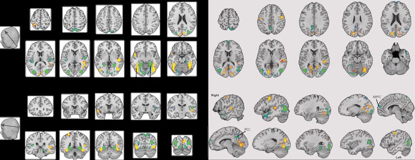
3.5. Imaging subspace projection
The reduced rank ridge regression (RRRR) approach is based on the projection of high dimensional
imaging data onto a subspace of lower dimension. Since this projection is linear, it is possible to visualise
the projections that are applied to imaging data to reconstruct the deep features (see Appendix A for more
details). As the hyperparameter tuning suggested optimal results with rank = 2 (see Figure 4), we display in
Figure 8 two projection maps, one per dimension of the reduced space (see also Table 9-10 in Supplementary
Material).
For the sake of clarity, we present the top 5% of the weights in these models. The first projection (left
panel) includes major bilateral clusters with opposite signs in the fusiform gyrus (including the fusiform face
area) and the parahippocampal pyrus (including the parahippocampal place area). These regions have been
associated with the face processing [55] and scene recognition [56], respectively. The second projection (right
panle) included major hubs in the motor cortex (bilateral) and association visual (bilateral) and auditory
(right) cortex. It also included large clusters across the posterior and anerior superior temporal cortex,
medial prefrontal cortex and the posterior cingulated cortex, which have been implicated in social cognition
and mentalization [57].
Figure 8: Three dimensional maps of the RRRR projections. Only the top 5% of the weights are visualised (minimal cluster
size: 25 voxels). Abbreviations: FG - fusiform gyrus; MPFC - medial prefrontal cortex; PHC - parahippocampal cortex; PCC
- posterior cingulated cortex.
20bioRxiv preprint first posted online Feb. 3, 2019; doi: http://dx.doi.org/10.1101/535377. The copyright holder for this preprint
(which was not peer-reviewed) is the author/funder, who has granted bioRxiv a license to display the preprint in perpetuity.
All rights reserved. No reuse allowed without permission.
To assess the functional meaning of the model in a quantitative manner, we used the web-based multi-
study decoder NeuroVault [58], which allows for the interpretation whole-brain patterns based on a large
database of neuroimaging studies. The top functional entries that were associated by the decoder with the
first projection were “face”, “recognition”, and “face recognition”. The second projection was most strongly
associated with the entries “vocal”, “production”, “saccades”, and “speech production”. These findings
support the notion that the models captured relevant features in the movies; namely, face presence in the
case of the first component and human speech in the case of the second component.
4. Discussion and future directions
In this work we have shown how to harness the richness of deep learning representations in neuroimaging
decoding studies. The potential benefit of the use of CNNs derived features i.e., fc7, is twofold. First, it is
possible to perform a task i.e., the regression from imaging data to fc7, that is more manageable, from the
dimensionality point of view, than a simple classification based solely on imaging data. We have shown in
Section 2.3 that this approach is useful and results in better classification performance, demonstrating how
to embed high-dimensional neuroimaging data onto a space designed for visual object discrimination. In
addition, using these networks for feature extraction allows us to extract stimuli representations by means
of an automatic procedure that does not require ground truth or supervision, and that may help to more
easily address certain unsupervised learning tasks.
ˆ it is possible that this
Regarding the good classification performance achieved with the predicted fc7,
is due to intrinsic redundancy and sparsity properties of CNN representations. A good analogy may be the
signal transmission process, in which some redundancies are introduced on purpose before transmitting the
information through the channel, so that the overall process can afford some losses. Also in this case the
CNN redundancy allows to obtain good classification performance despite the fact that the reconstruction
ˆ is not perfect.
fc7
In brain imaging literature, and in a broader sense in all biomedical engineering fields, from neuroscience
to genetic, there are plenty of multivariate linking methods, with different formulations and training strate-
gies. In this work we have compared some of the most widely used multivariate approaches, and our results
indicate that the best performance for the type of data we considered is obtained by RRRR method. Given
the large amount of time points on which it has been tested, these results are reliable and we thus recommend
the use of RRRR in the context of combining fMRI data and such deep computational models.
The reliability of the proposed method is clearly demonstrated by the adopted inter-subject approach in
the movie dataset. While most of the works present in literature rely on single subject analyses in very con-
trolled stimulation settings, we decided to also consider, alongside with the static image dataset, movie clips
with free viewing. In addition to this, we performed training and testing using separate movie subsets, testing
21You can also read


