Forecasting forecaster accuracy: Contributions of past performance and individual differences

Judgment and Decision Making, Vol. 16, No. 2, March 2021, pp. 323–362

 Forecasting forecaster accuracy: Contributions of
 past performance and individual differences

 Mark Himmelstein∗† Pavel Atanasov‡ David V. Budescu§

 Abstract

 A growing body of research indicates that forecasting skill is a unique and stable
 trait: forecasters with a track record of high accuracy tend to maintain this record. But
 how does one identify skilled forecasters effectively? We address this question using
 data collected during two seasons of a longitudinal geopolitical forecasting tournament.
 Our first analysis, which compares psychometric traits assessed prior to forecasting,
 indicates intelligence consistently predicts accuracy. Next, using methods adapted from
 classical test theory and item response theory, we model latent forecasting skill based
 on the forecasters’ past accuracy, while accounting for the timing of their forecasts
 relative to question resolution. Our results suggest these methods perform better at
 assessing forecasting skill than simpler methods employed by many previous studies.
 By parsing the data at different time points during the competitions, we assess the
 relative importance of each information source over time. When past performance
 information is limited, psychometric traits are useful predictors of future performance,
 but, as more information becomes available, past performance becomes the stronger
 predictor of future accuracy. Finally, we demonstrate the predictive validity of these
 results on out-of-sample data, and their utility in producing performance weights for
 wisdom-of-crowds aggregations.
 Keywords: forecasting, individual differences, item response models, longitudinal
 analysis, skill assessment, wisdom-of-crowds, hybrid forecasting competition
 ∗ Department of Psychology, Fordham University. https://orcid.org/0000-0001-8681-0482.
 † Correspondence Email: mhimmelstein@fordham.edu
 ‡ Pytho LLC. https://orcid.org/0000-0002-9963-7225.
 § Department of Psychology, Fordham University. https://orcid.org/0000-0001-9613-0317.

 323

Judgment and Decision Making, Vol. 16, No. 2, March 2021 Forecasting accuracy

1 Introduction
From ancient oracles to modern prediction markets, humanity has long been fascinated
by the prospect of predicting future events. While data-driven approaches to prediction
have grown in popularity, human forecasting remains important, especially in data-sparse
settings. Human forecasting is a unique psychological process. Unlike strictly intellective
tasks, driven entirely by domain-specific knowledge, or judgmental tasks that relate to
preferences, values and opinions, forecasting features a combination of intellective and
judgmental processes (Fan et al., 2019; Stael von Holstein, 1970; Wallsten & Budescu,
1983). What makes a good forecaster? Is it someone who is highly knowledgeable regarding
the particular subject being forecasted? Someone who excels at probabilistic reasoning and
inference? Perhaps a combination of both? Or perhaps neither, and forecasting is a unique
skill unto its own.
 We address these questions by examining data collected during several geopolitical
forecasting tournaments. Forecasting tournaments are a relatively recent innovation in
which participants make repeated forecasts for numerous events over a specified period of
time, and the winners are determined by objective scoring rules that reflect the forecasts’
accuracy (Tetlock et al., 2014). These tournaments provide an information-rich research
environment for studying processes related to human forecasting, including the correlates
of forecasting skill.

1.1 Forecasting Tournaments
In 2011, the Intelligence Advanced Research Projects Activity (IARPA) launched the Ag-
gregative Contingent Estimation (ACE) program (Tetlock et al., 2014). The goal of the ACE
program was to develop highly accurate forecasting systems by invoking wisdom-of-crowds
(WoC) principles (Budescu & Chen, 2014; Davis-Stober et al., 2014; Surowiecki, 2005).
The WoC predicts that crowdsourced aggregations of judgments of many forecasters will
substantially outperform individual forecasters, including highly trained experts. To incen-

 We would like to thank the entire SAGE team for their dedication to the HFC and support of our research.
 This research is supported by the Office of the Director of National Intelligence (ODNI), Intelligence
Advanced Research Projects Activity (IARPA), via 2017-17071900005. The views and conclusions contained
herein are those of the authors and should not be interpreted as necessarily representing the official policies,
either expressed or implied, of ODNI, IARPA, or the U.S. Government. The U.S. Government is authorized
to reproduce and distribute reprints for governmental purposes notwithstanding any copyright annotation
therein.
 Copyright: © 2021. The authors license this article under the terms of the Creative Commons Attribution
3.0 License.
 ∗ Department of Psychology, Fordham University. https://orcid.org/0000-0001-8681-0482.
 † Correspondence Email: mhimmelstein@fordham.edu
 ‡ Pytho LLC. https://orcid.org/0000-0002-9963-7225.
 § Department of Psychology, Fordham University. https://orcid.org/0000-0001-9613-0317.

 324

Judgment and Decision Making, Vol. 16, No. 2, March 2021 Forecasting accuracy

tivize participation, ACE was structured as a series of forecasting competitions in which
participants forecasted the same events and were assessed by predetermined criteria.
 Multiple research groups were recruited and tasked with developing forecasting systems.
Each group developed their own platform and hosted a separate forecasting tournament
based on an identical set of questions, which covered several domains with forecasting
horizons ranging from a few weeks to several months. One such research group was the
Good Judgment Project (GJP, Mellers et al., 2014). A key feature of the GJP approach was
identifying highly skilled individual forecasters, or Superforecasters (Mellers, et al., 2015b;
Tetlock & Gardner, 2016). By identifying these individuals, GJP was able to both cultivate
their performance and develop weighted aggregation methods that relied more heavily on
their judgments without sacrificing the benefits of the WoC approach (Atanasov et al., 2017;
Budescu & Chen, 2014; Chen et al., 2016; Karvetski et al., 2013).
 In 2017, IARPA launched a follow-up tournament: the Hybrid Forecasting Competition
(HFC) (IARPA, 2018). HFC was a competition between three research groups, whose
goal was to find effective methods for combining human judgment with machine models in
forecasting. HFC was divided into two seasons, structured as Randomized Controlled Trials
(RCTs)1 with forecasters randomly assigned to research groups at the start of each season.
Each season lasted six to eight months. The authors were members of the Synergistic
Anticipation of Geopolitical Events (SAGE) research group (Morstatter et al., 2019).
 This RCT structure raised a new challenge to the crowd prediction approach. As
researchers had only a limited time window to identify skilled forecasters, it was critical to
do so as early as possible and develop optimal weighting schemes based on the information
available at any given moment. Although the constraints of the RCT structure did not allow
research groups to gain an edge by recruiting superior forecasters, they provided a more
controlled research environment. As such, these tournaments provide an ideal opportunity
to generalize and extend past results regarding individual forecasting performance.
 What constitutes a skilled forecaster? Are there certain traits that reliably identify skilled
forecasters? If so, how can we leverage and balance these traits in the presence or absence
of information on past forecasting performance? Our goal is to address these questions and
understand the best ways to measure and identify forecasting skill by using data collected
by the SAGE research group during the two seasons of the HFC program.

1.2 Individual Forecaster Assessment
A critical result from the GJP research was that forecasting skill is a relatively stable trait
(Mellers, et al., 2015a; Mellers, et al., 2015b; Tetlock & Gardner, 2016). Forecasters who
have performed well in the past, and forecasters who are more active and engaged, are more
likely than others to produce accurate forecasts. In other words, it is possible to reliably
predict future accuracy from past performance and task engagement (e.g., Chen et al. 2016;
 1We use the terms “season”, “study”, and “RCT” interchangeably throughout.

 325

Judgment and Decision Making, Vol. 16, No. 2, March 2021 Forecasting accuracy

Mellers, et al., 2015b). Psychometric theory provides methods for measuring trait levels
across individuals.
 Before describing these psychometric methods, it is important to define our usage
of certain terms. Accuracy is a property of an actual forecast — namely, how well it
represented the eventual outcome. Ability or skill is a latent trait that drives the degree
to which forecasters predictably vary in accuracy. Finally, performance is a general term
representing a forecaster’s empirical contributions during a forecasting competition. This
term refers primarily to empirical estimates of ability, but it can also include the extent of
active participation.
 The distinction between performance and skill is subtle, but important. Performance is
a function of an individual’s behavior as well as the task. If an athlete is playing one-on-one
basketball and scores a basket, she is awarded two points. The total score at the end of
a game is a measure of player performance, which can be compared with an opponent’s
performance to determine a winner. If these two players were to play again, it is highly
unlikely the game would end with the exact same score; and if a players’ opponent changed,
it is even less likely the score would be repeated. As this example suggests, performance is
local, specific and unreliable — it varies from elicitation to elicitation — as other contextual
and/or stochastic factors influence the result as well. Skill, on the other hand, is a global and
stable latent ability, or trait, intrinsic to an individual. Traits are not directly observable, but
they are thought to predict behavior, and thus performance. Performance can be considered
an unbiased estimator of skill, but only when certain assumptions are met.

1.3 Psychometric Theory
In classical test theory (CTT), observed performance is considered a combination of an
individual’s “true” level on a given trait, and residual error (Bandalos, 2018; Lord &
Novick, 1968; Novick, 1966). The canonical CCT model, where X refers to an observed
score, T an individual’s unobservable true trait level, and E to residual error, is given as:

 = + (1)

 This equation is mirrored in the literature on forecasting, which partitions measures of
average individual accuracy into skill components perturbed by residual error (Mandel &
Barnes, 2014; Murphy, 1973; Wallsten & Budescu, 1983). If residual error is assumed to
be random with a mean of 0, an observed score is an unbiased estimate of the trait level, as
measured on the scale of the performance metric. Several, often unrealistic conditions are
required for this assumption to hold. For example, all forecasters must either forecast the
same questions, or variation in question difficulties must be accounted for. In the context of
longitudinal forecasting, the timing of a forecast also plays a role: how does the timing of
forecasts about the same event influence difficulty? Addressing these issues is critical for
applying the classical psychometric model to a forecasting tournament in which participants
self-select when and which events to forecast.

 326

Judgment and Decision Making, Vol. 16, No. 2, March 2021 Forecasting accuracy

 An alternative psychometric approach, designed in part to address these issues, is known
as Item Response Theory (IRT) (Embretson & Reise, 2013; Lord & Novick, 1968). Whereas
in CTT, items are typically treated as equivalent components of a total score, IRT is based on
the principle that different items carry unique information about the trait they are supposed
to measure. Originally developed for measuring trait levels based on educational tests,
the most well-known IRT models estimate the conditional probability that an individual
provides a certain response to each item, given their level on the relevant trait as well as
parameters that define each item’s diagnostic properties.2 One of the most common IRT
models is the two-parameter logistic model. The two parameters refer to each item’s two
diagnostic parameters: difficulty (b) and discrimination (a). The trait level of participants
is represented by a person-specific parameter, . Where is a binary response variable
for person j on item i, this model is:
 1
 ( = 1| , , ) = (2)
 1 + − ( − )
In this model, represents the location on the latent trait scale such that, for item i, a
person with = will answer the item correctly with probability = .5, while represents
a steepness parameter which determines how well item i discriminates values of near
 . The scale for is computationally indeterminate. Conventionally it is scaled such that
 ∼ N (0, 1), and the scale for b is determined by the scale for . In this model, each item
can be considered to have its own unique function, known as an item response function.
 Applied to forecasting, one can think of the standard classical test theory model as
producing a direct measure of skill, representing the mean accuracy of all forecasts a
forecaster makes, where all forecasts are assigned equal weight, regardless of the timing or
event being forecasted. One can, likewise, think of measures based on IRT as a weighted
average of a forecasters’ accuracy across all of their forecasts, where the weights are a
function of the event (or item) specific parameters (see Bo et al., 2017). As such the IRT
measures should be more sensitive to the specific events people choose to forecast.

1.4 Longitudinal Forecasting
A unique problem in a longitudinal forecasting setting is the effect of time. Since all
forecasting questions have a pre-determined resolution time, forecasting gets easier as time
passes. In some cases, this reflects the structure of the forecasting problem, as options are
restricted or ruled out, similar to how the number of baseball teams that can theoretically
win the World Series is reduced as other teams are eliminated during earlier playoff rounds.
In other cases, this simply reflects the accumulation of information over time, such as a
sudden shortage of a given commodity increasing its price. Figure 1 demonstrates changes
in average accuracy over time across all HFC questions that were at least 12 weeks in
 2There are various IRT models that vary, primarily, with respect of how many (and which) item parameters
they include.

 327

Judgment and Decision Making, Vol. 16, No. 2, March 2021 Forecasting accuracy

duration and demonstrates how empirical accuracy improved monotonically as a function
of time to resolution.
 Accounting for timing represents a non-trivial problem in assessing a forecaster’s skill.
Merkle et al. (2016) used an IRT-based approach to adjust for the effect of time on accuracy,
however they did not explicitly link their results to proper scoring rules. Bo et al. (2017)
demonstrated that IRT methods can be linked to proper scoring rules, however they did
not consider changes in accuracy over time. We demonstrate that it is possible to combine
these methods and link an IRT-based approach to proper scoring rules while accounting for
temporal changes in forecasting difficulty. We also demonstrate a novel approach to direct
accuracy assessment that can account for temporal changes in difficulty, which bears more
resemblance to CTT methods.

 3
Average Accuracy

 2
 Season
 1
 2
 1

 0

 12 11 10 9 8 7 6 5 4 3 2 1

 Weeks Until Resolution
Figure 1: Average accuracy of forecasts as a function of time for all questions of at least 12
weeks in duration. Average accuracy refers to normalized accuracy scores (see methods).
For a binary forecasting question, normalized accuracy of 0 represents a probability of exactly
.5 assigned to the correct option. Higher values represent more accurate forecasts.

 In addition to expanding on previous studies that have applied IRT models to probability
judgments (Bo et al., 2017; Merkle et al., 2016), we also intend to demonstrate their
practical applications. Both previous studies relied on the same dataset generated by
GJP. These data were based on a subset of questions with especially high response rates,
which were selected to avoid potential complications related to data sparsity. However, as
Merkle et al. (2017) point out, question selection is an important and frequently neglected
dimension of performance. Focusing only on the most popular questions potentially limits
the generalizability of these foundational results. We apply IRT models across all forecasting
questions included in HFC, and demonstrate their practical applications even when less
popular questions are included.

 328

Judgment and Decision Making, Vol. 16, No. 2, March 2021 Forecasting accuracy

1.5 The Cold Start Problem
One inherent problem when using past performance to identify high ability forecasters
is that this information is not immediately available. Without performance information
available to estimate skill, these approaches are of no use. This is an example of the cold
start problem, which is a common issue in systems which use past behavior to predict future
behavior (Lika et al., 2014; Schein et al., 2002).
 Fortunately, results generated by the GJP indicate that forecasting ability can be modeled
using other trait measures that are accessible even in the absence of past performance infor-
mation. Mellers, et al. (2015a) found that general intelligence — particularly quantitative
reasoning ability (Cokely et al., 2012) and reflective thinking (Baron et al., 2015; Frederick,
2005) — along with open mindedness (Stanovich & West, 1997) and relevant subject knowl-
edge were particularly helpful in predicting forecasting skill. Moreover, skilled forecasters
tended to be highly coherent, i.e., their judgments followed the axioms of propositional
logic, and well calibrated, i.e., they assigned probabilities to events which correspond, on
average, with the actual outcomes (Karvetski et al., 2013; Mellers et al., 2017; Moore et al.,
2016). Coherence and calibration have been found to be important factors in other tasks
related to probability judgment as well (Fan et al., 2019). Other approaches to early skill
identification have focused on proxy measures for accuracy available before forecasting
questions resolve (Witkowski, et al., 2017), or on behaviors observable in real-time, such
as forecast updating (Atanasov et al., 2020).
 Cooke’s method (also known as the “classical model”) in which one administers a
series of domain specific general knowledge calibration questions provides an alternative
solution to the cold start problem. The participants provide responses and rate their degree of
confidence in those responses, prior to eliciting any actual forecasts (Aspinall, 2010; Colson
& Cooke, 2018; Hanea et al., 2018). While domain knowledge can be a helpful predictor
of forecasting accuracy (Mellers, et al., 2015a), these confidence ratings also provide
a measure of calibration by comparing a forecaster’s confidence to actual performance
on these domain questions. Calibration is an important component of any probability
judgment, and people tend to be overconfident in their judgments about their performance
to both general knowledge questionnaires (Brenner et al., 1996) and forecasts (Moore et al.,
2016).

1.6 Research Questions and Hypotheses
Our goal is to determine how to best identify high performing forecasters and to demon-
strate how different sources of information can be utilized to achieve this goal. We seek
to demonstrate how helpful individual difference measures are by themselves when no past
performance information is available, and how much benefit is added over time as perfor-
mance information becomes available. Past studies have shown both sources of information
can identify forecasting skill, but no study has shown how they complement each other, or

 329

Judgment and Decision Making, Vol. 16, No. 2, March 2021 Forecasting accuracy

how the relative importance of the sources changes as performance data accumulate. To
answer this question, we first generalize past findings that have demonstrated the utility
of performance and individual difference information separately, before examining their
joint contributions at various time points. We further synthesize the IRT approaches of
Merkle et al. (2016) and Bo et al. (2017) to link our model’s performance-based estimates
of forecasting ability to proper scoring rules, while accounting for changes in difficulty for
forecasting different events over time, as well as propose a new time-sensitive approach to
direct assessment. The first three hypotheses pertain to generalization of prior research,
while the last three are new.
 Hypothesis 1. Individual difference measures of intelligence, cognitive style, domain
knowledge and overconfidence in domain knowledge (calibration) will predict accuracy of
future forecasts. (Generalization)
 Hypothesis 2. Empirical measures of forecaster ability based on the accuracy of their
forecasts will be stable over time. (Generalization)
 Hypothesis 3. IRT-based estimates of forecasting skill (based on past performance)
will predict accuracy of future forecasts better than direct skill measures. (Generalization)
 Hypothesis 4. Adjusting for forecast timing relative to event resolution will improve
direct ability assessment methods. (New hypothesis)
 Hypothesis 5. As information about performance becomes available, these performance-
based skill estimates will surpass individual difference measures assessed in advance at
predicting accuracy of future forecasts. (New hypothesis)
 Hypothesis 6. Performance weights using a combination of individual difference
information and IRT-based skill assessment will optimize wisdom-of-crowds aggregation
relative to weights that combine direct skill assessment measures and individual differences.
However, weights that combine direct skill assessment measures and individual differences
will still perform better than weights that rely on individual differences alone. (New
hypothesis)

2 Study 1: HFC Season 1
2.1 Methods
Sample Information. The first season of the HFC relied on a sample of volunteer recruits
who were randomly assigned to the various research groups. In total, 1,939 participants
were assigned to SAGE and filled out an intake battery of psychometric surveys (see details
below). However, only 559 of them participated in active forecasting. Their mean age
was 43.11 (SD = 13.93) and 16.1% were women. A subset of 326 of these 559 forecasters
made at least five total forecasts. We used this sample (the “core sample”), to reduce noise
introduced by low activity participants. Their mean age was 43.67 (SD = 14.12) and 15.0%
were women. The remaining 1,380 (the “supplementary” sample) registered and completed
the intake surveys but did not forecast. Their mean age was 42.90 (SD = 14.35) and 18.7%

 330

Judgment and Decision Making, Vol. 16, No. 2, March 2021 Forecasting accuracy

were women. Although these participants provided no forecasting data, they did provide
useful data for fitting measurement models of the elicited trait measures.
 Procedure. The core sample forecasted 188 geopolitical questions, generated by
IARPA, between March and November of 2018. Forecasters were eligible to forecast
on as many, or as few, questions as they liked, and could make and revise forecasts as fre-
quently as they liked while a question was open for forecasting. The mean question duration
was 67.97 days, SD = 49.41. The mean number of questions participants made at least one
forecast on was 14.10, SD = 26.29. The mean number of forecasts that participants made
per question was 2.15, SD = 3.12. Questions used C mutually exclusive and exhaustive
response options(2 ≤ ≤ 5), and forecasters were informed exactly how the ground truth
(or resolution) of each item would be determined. Information on all 188 questions is
included in the supplementary materials.
 For each question, forecasters estimated the probability of events associated with each
response option occurring. The sum of all probabilities assigned across all C response
options for a question was constrained to total 100. There were three types of questions:
88 binary questions (47%), 15 multinomial unordered (8%), and 85 multinomial ordinal
questions (45%). Binary questions had only two possible response options (e.g. Yes or
No). Multinomial (unordered) questions had more than two possible response options, with
no ordering (e.g., a question about the outcome of an election between four candidates).
Ordinal questions had more than two possible response options with a meaningful ordering
(e.g., bins corresponding to the price of a commodity on a given date). Table 1 includes
examples of all three types of question.
 Individual Differences. An intake battery was administered to all 1,939 registered
participants in the volunteer sample prior to beginning forecasting activity, including those
who did not participate in forecasting. The surveys were administered in one session prior to
assignment to the SAGE platform (mean testing time = 51 minutes). All scales administered
are included in the supplementary materials. There were three broad classes of measures:
 Intelligence. We used four performance-based scales related to fluid intelligence and
quantitative reasoning. A six-item version of the Cognitive Reflection Test consists of
multiple-choice mathematical word problems with intuitively appealing distractor options.
The version administered contained three items form the original version (Frederick, 2005)
and three items from a more recent extension (Baron et al., 2015). The Berlin Numeracy
Scale is a 4-item scale which measures numerical reasoning ability, including statistics
and probability (Cokely et al., 2012). A 9-item Number Series completion task, in which
participants are asked to complete sequences of numbers which fit an inferable pattern
(Dieckmann et al., 2017). An 11-item Matrix Reasoning Task, similar to Raven’s Progres-
sive Matrices (Raven, 2000), but drawn from a large bank of computer-generated items
(Matzen et al., 2010).
 Cognitive Styles. Two self-report measures were administered. Both used 5-point Likert
response scales. Actively Open-Minded Thinking is an 8-item scale designed to measure

 331

Judgment and Decision Making, Vol. 16, No. 2, March 2021 Forecasting accuracy

 Table 1: Forecasting Question Examples

Question Type Question Resolution Criteria Option 1 Option 2 Option 3 Option 4 Option 5

 Question will be
 resolved if the
 Will the WHO
 World Health
 declare a Public
 Organization (WHO)
 Health Emergency
 declares a PHEIC
Binary of International Yes No –~ – –
 via WHO Statements
 Concern
 from the International
 (PHEIC) before 1
 Health Regulations
 September 2018?
 (IHR) Emergency
 Committee

 Who will win Andrés
 Mexico’s presidential Ricardo José
 Mexico’s Manuel Another
Unordered election is scheduled for Anaya Antonio –
 presidential López candidate
 1 July 2018 Cortés Meade
 election? Obrador

 Between More than Between
 What will be the Question will be resolved
 Less $,120 $,160 $,190 More
 daily closing price of using the London
Ordinal than and but less and than
 gold on 5 September Bullion Market
 $120 $,160, than $1,230, $1,230
 2018 in USD? Association (LBMA)
 inclusive $1,190 inclusive

willingness to reason against one’s own beliefs (Mellers et al., 2015a). Need for Cognition
is an 18-item scale designed to measure willingness to engage in effortful thinking and
reflective cognition (Cacioppo & Petty, 1982).
 Political Knowledge. A 50-item true/false quiz testing participants’ knowledge regarding
current geopolitical events was administered. The questions covered a wide range of
domains and geographic regions. In addition to answering the quiz, participants rated their
confidence in their responses. This confidence judgment provided an application of Cooke’s
method of using calibration between confidence and accuracy for predicting forecasting
skill (Aspinall, 2010; Colson & Cooke, 2018). An Overconfidence score was calculated,
across all 50 items for each forecaster as: = ( ) −
 ( ).
 Trait Measurement Models. The simplest approach to applying the individual differ-
ence measures is to treat each scale as a unique predictor. To reduce the dimensionality
of these data, we fit a confirmatory factor model on the supplementary sample and used
these parameters to estimate factor scores for the core participants for general intelligence
and cognitive style (see above). Details and results of this procedure are included in the
supplementary materials.
 Forecast Accuracy. The accuracy of each forecast was measured using the Brier Score,

 332

Judgment and Decision Making, Vol. 16, No. 2, March 2021 Forecasting accuracy

a metric developed to measure the accuracy of weather forecasts (Brier, 1950). The Brier
score is a strictly proper scoring rule, in that the strategy to optimize it is to provide a
truthful account of one’s beliefs regarding the probability of an event (Gneiting & Raftery,
2007; Merkle & Steyvers, 2013). The Brier score contrasts a forecast and the eventual
ground truth. For an event with C response options (or bins, b), the Brier score is the sum
of squared differences between the forecasted probability for a given bin — which can
range from 0 to 1 — and the outcome of that bin — which takes on a value of 1 if the
event occurred and 0 if the event did not occur. Brier scores range from 0 (perfect accuracy)
to 2 (worst case, most inaccurate). Formally:
 
 Õ
 = ( − ) 2 (3)
 =1

In the binary case, with two possible response options, where represents the forecasted
value of the ground truth option, the formula is reduced to:

 = ( − 1) 2 + ((1 − ) − 0) 2 = 2(1 − ) 2 = 2( − 1) 2 (4)

 There is a wrinkle regarding the scoring of ordinal questions. Consider the example in
Table 1 and assume that the correct option winds up being Option 5, the price of gold >
$1,230. Consider two forecasts which are identical, except in once case a probability of .75
is assigned to Option 4, and in the other, a probability of .75 is assigned to Option 1. Since
Option 4 is “closer” to Option 5, the forecast which assigns higher probability to Option 4
than Option 1 should be considered superior. The standard Brier score is agnostic to this
distinction. To correct this shortcoming, Jose et al. (2009) defined a variant of the Brier
score which accounts for ordinality in response options. The Ordinal Brier score considers
all ( − 1) ordered binary partitions of the C bins, calculates a score for each partition, and
averages them. The Ordinal Brier score formula can be written:
 −1
 " 
 #2
 2 Õ Õ Õ
 Ordinal BS = ( ) − ( ) (5)
 − 1 =1 =1 =1

 Skill Measurement. The ability of individual forecasters is typically assessed by
averaging the Brier scores of all of their forecasts (Bo et al., 2017; Mellers et al., 2015a;
Merkle et al., 2016), a form of direct assessment. However, since the Brier score measures
squared errors across all events associated with a forecasting question, its distribution is
heavily right-skewed, meaning it is increasingly sensitive to higher levels of inaccuracy.
Put another way, it will over-weight large errors relative their expected frequency, which is
not a desirable property for measuring the accuracy of individual forecasters. It also means
standard modeling assumptions, such as normality and homoscedasticity of residuals, will
be violated when Brier scores are used as criterion variables in comparative analyses.
 Merkle et al. (2016) implicitly address this by directly referencing the probability as-
signed to the ground truth as their accuracy criterion, rather than the Brier score. Bo et al.

 333

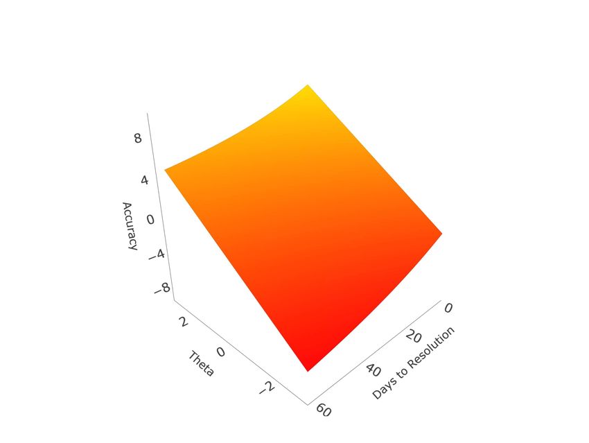
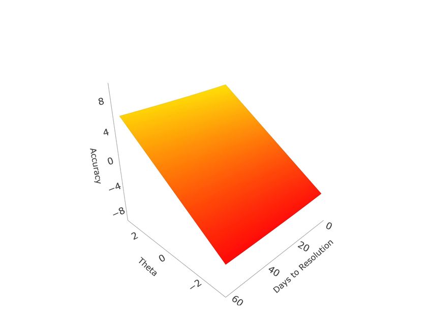
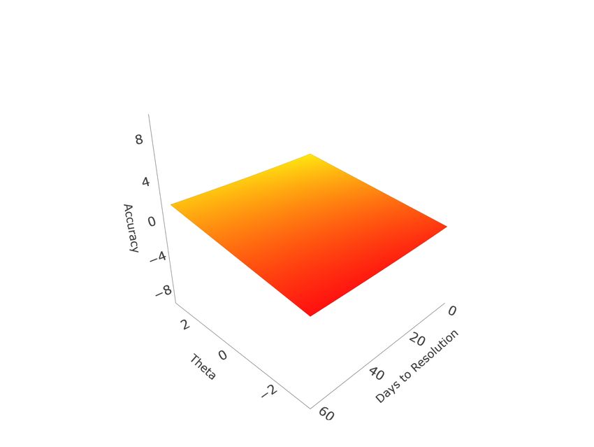
Judgment and Decision Making, Vol. 16, No. 2, March 2021 Forecasting accuracy

(2017) further note, as can be seen from equation 4, that for binary items the probability
assigned to ground truth directly maps onto the Brier score via a quadratic link, though
this is not the case when a forecasting question involves more than two events. In such
cases, different forecast distributions can produce identical Brier scores. However, Brier
scores can be mapped to unique values on the [0,1] scale in the reverse direction using the
following formula, with higher values instead reflecting more accurate forecasts:
 r
 
 = 1 − (6)
 2
This reverse transformation (note than when = 2 this formula reproduces ) permits us
to generalize the methods of Merkle et al. (2016) and Bo et al. (2017) to questions where
 > 2.
 Time and Difficulty. Taking a simple mean of accuracy across forecasts to produce
a standard direct skill assessment ignores the effects of time. This was one of the key
factors motivating Merkle et al.’s (2016) application of IRT models. They proposed two
approaches to transform accuracy scores to satisfy model assumptions: using a probit link
to normalize probability values, or discretizing scores into ordered bins. While Merkle et al.
(2016) recommended, and Bo et al. (2017) opted for, the latter approach, this was driven by
concerns related to unique patterns of dispersion in their data, with high densities of forecast
values at 0, .5, and 1. Due to the large proportion of multinomial and ordinal forecasts
that had to be back-transformed from Brier scores (see eq. 6), our data was more evenly
dispersed. Thus, we pursued the probit approach, which both requires fewer parameters
and preserves information. For our IRT approach, we adopt Merkle et al.’s (2016) probit
model, where Normalized Accuracy is defined as:

 r !
 
 Normalized Accuracy = ( ) = 1 − (7)
 2

 As a direct a transformation of Brier scores, normalized accuracy does not have a precise
intuitive interpretation. One way to conceptualize normalized accuracy is that 0 represents
a Brier score of 0.5, which corresponds to a probability of .5 assigned to the correct option
for a binary question. Higher normalized accuracy values represent more accurate forecasts.
The normalized accuracy IRT model is specified as

 Normalized Accuracy = 0 + ( 1 − 0 ) − 2 + + , (8)

where 0 represents the lower asymptote on an item’s expected accuracy as time to res-
olution increases, 1 the upper asymptote on expected accuracy at resolution, 2 the rate
of change in difficulty over time3, an item’s factor loading (which can be converted into
 3Note that we follow Merkle et al. (2016) in allowing 0 and 1 to vary by item, but not 2 . Thus, 2
represents the mean (common) rate of change in difficulty over time between 0 and 1 for all questions.

 334

Judgment and Decision Making, Vol. 16, No. 2, March 2021 Forecasting accuracy

the IRT discrimination parameter, see Merkle et al., 2016), and a person’s ability level.
Although this model uses a continuous outcome, it resembles the four-parameter logistic
IRT model, which is an extension of the two-parameter model for binary outcomes with
additional parameters for a lower asymptote (representing guessing behavior) and upper
asymptote (representing irreducible uncertainty) (Barton & Lord, 1981; Loken & Rulison,
2010). Figure 2 presents hypothetical item response functions based on this model. By
varying 0 and 1 , we illustrate different ways forecast timing can affect accuracy; and
by varying we illustrate how questions with higher factor loading better discriminate
forecaster ability. The slopes of the response surface illustrate the relative sensitivity of
accuracy to the two factors, time and ability, in the various cases.
 We also consider two additional approaches to direct skill assessment. The first vari-
ation, simple standardized accuracy, standardizes forecasters’ mean accuracy within each
question, to account for differences in difficulty across questions. This is the most similar
metric to what Mellers et al. (2015a) and Bo et al. (2017) used as a criterion. The key
difference in our approach is that, rather than standardizing Brier scores, we standardize the
normalized accuracy scores (eq. 7). This serves to both help satisfy subsequent modeling
assumptions and allow for more direct comparison with the IRT approach.
 The second approach accounts for the effect of time on direct skill assessment by
employing the following hierarchical model:

 Normalized Accuracy = 00 + 0 + 0 + 1 log( ) + (9)

In this model, 0 serves the same function as the T term in the CCT model (eq 1): an
estimated forecaster-specific “true score”. However, in addition to error, in this model 0 is
also conditional on ( ) for each forecast, as well as 0 , which represents the average
accuracy of each question, across all forecasters. This effectively accounts for the difficulty
(or more precisely, easiness) of each question. As such, 0 is an estimated mean forecaster
accuracy which accounts for both question difficulty and the effect of time. This model
represents a compromise between the IRT and simple standardized approaches, in that it
estimates fewer parameters and is more computationally efficient than the IRT approach,
but still includes adjustments for question difficulty and the effect of time.
 Metric Scales. The three metrics are on slightly different, but similar scales. The
simple and hierarchical ability assessments are based on the actual normalized accuracy
scale. Because question difficulty is accounted for, an average forecaster would be expected
to have a score of 0 on both metrics, with better forecasters having higher scores and weaker
forecasters having lower scores, though the units do not have a clear intuitive interpretation.
On the other hand, the IRT model requires to be scaled for model identification. This
makes the resulting metric more meaningful, as it is interpretable as estimated z-scores.
This is an advantage of the IRT approach.

 335

Judgment and Decision Making, Vol. 16, No. 2, March 2021 Forecasting accuracy

 0 = −0.5, 1 = 0.5, = 0.5 0 = −0.5, 1 = 0.5, = 2

 0 = −4, 1 = 4, = 0.5 0 = −4, 1 = 4, = 2

Figure 2: Four hypothetical item response functions. Top row represents questions where
difficulty is relatively constant over time, bottom row where difficulty is very sensitive to timing.
Left column represents questions which poorly discriminate forecasters of differing ability
levels, right column represents questions which discriminate forecasters of differing abilities
well (Note that 2 is held constant at 6.63, the empirical estimate for Season 1).

 Programming. All data analysis was performed with the R statistical computing
platform (R Core Team, 2020). Hierarchical models were fit with the lme4 package (Bates
et al., 2015). Item response models were programmed in Stan (Stan Development Team,
2020b) and interfaced via RStan (Stan Development Team, 2020a). All programs are
available in the supplementary materials.

2.2 Results and Discussion
Individual Differences. We began by probing the results of each intake scale on the
data obtained from the supplementary sample (n = 1,380). Cronbach’s ranged between
moderate and good for the Cognitive Reflection Test (.80), Berlin Numeracy (.70), Number

 336

Judgment and Decision Making, Vol. 16, No. 2, March 2021 Forecasting accuracy

Series (.73), and Need for Cognition (.85); moderate for Matrix Reasoning (.56) and Actively
Open-Minded Thinking (.64) and low for Political Knowledge (.44)4. Measurement model
results for intelligence and cognitive style based on these scales are in the supplementary
materials.
 We removed one item from the Political Knowledge quiz because all participants an-
swered it correctly. Overconfidence scores for the remaining 49 items in the core sample
(n = 326) had mean = 0.02, SD = 0.09, where a score of 0 denotes perfect calibration,
positive scores reflect over-confidence, and negative scores under-confidence. We consider
forecasters who were within half a standard deviation from 0 as relatively well calibrated,
forecasters who were more than half a standard deviation above 0 as over-confident, and
those who were more than half a standard deviation below 0 as under-confident. We found
that 133 (41%) were well-calibrated, 127 (39%) were overconfident, and only 66 (20%)
were under-confident. Overall, participants were twice as likely to be overconfident than
under-confident, a result which is a typical finding (Brenner et al., 1996).
 Ability Measures. Figure 3 displays the distributions and correlations between the
3 ability measures (simple, hierarchical, IRT). The three accuracy measures were highly
correlated across the full dataset (326 forecasters and 188 questions). We next split the
data into two halves (the first 94 questions to resolve, and the remaining 94), to test the
temporal stability of these metrics. Table 2 contains correlations for each measure between
and within time periods. These results are consistent with Hypothesis 2, that empirical
assessments of forecaster ability based on accuracy are stable over time.

Table 2: Correlations between accuracy measures between and within two sets of 94 fore-
casting questions from Season 1 (N = 326 forecasters). Between time correlations in italics,
with comparisons of the same metric across time in bold.

 T1 T2
 Simple Hierarchical IRT Simple Hierarchical
 Hierarchical .72
 T1
 IRT .71 .83
 Simple .36 .34 .38
 T2 Hierarchical .29 .40 .41 .82
 IRT .30 .39 .36 .79 .92

 Individual Differences Predict Estimated Ability. Table 3 displays the correlations
between the ability measures and various scales and the demographic variables. As in
Mellers et al. (2015a), variables related to general intelligence, cognitive style, domain
 4One possible explanation for this result is the wide range of domains and geographic regions covered
by the questions. We opted to retain this metric both as a control variable for the calibration scale based on
political knowledge, and as our only assessment of domain knowledge.

 337

Judgment and Decision Making, Vol. 16, No. 2, March 2021 Forecasting accuracy

 Simple Hierarchical IRT
 1.00
 0.75

 Simple
 Corr: Corr:
 0.50
 0.834 0.782
 0.25
 0.00
 1.0

 Hierarchical
 0.5
 0.0
 Corr:
 0.880
 −0.5
 −1.0

 2

 0

 IRT
 −2

 −4
 −1 0 1 2 −1.0 −0.5 0.0 0.5 1.0 −4 −2 0 2

Figure 3: Scatterplot matrix of three ability assessments (simple, hierarchical, IRT) across
all forecasters from Season 1 (n = 326).

knowledge, and education show the highest correlations with ability. Overall, the correla-
tional pattern is consistent with these past findings for each of the ability measures, with
some minor differences. For example, in our results, CRT, rather than matrix reasoning,
shows the highest correlation with ability. However, Mellers et al. (2015a) used mean
standardized Brier scores, not normalized accuracy, and accounted differently for forecast
timing. It is possible that these methodological differences account for some of these minor
discrepancies.
 Individual Differences Predict Accuracy. To demonstrate the relationship between
individual differences and forecast accuracy, we fit a hierarchical model with intelligence,
cognitive style, political knowledge, overconfidence, age, gender, and education predicting
the normalized accuracy scores for each forecast, with random intercepts for forecasters and
questions, and controlling for (the log of) time remaining until resolution. We compared
this model to a simplified (nested) model with only these random intercepts and the time
covariate. A likelihood ratio test revealed individual differences significantly predict nor-
malized accuracy beyond the effect of time ( 2 (7) = 35.11, < .001, 2 = .14, where 2
is based on the reduction in forecaster random intercept variance attributable to individual
differences using the procedure outlined by Raudenbush & Bryk, 2002). These results are
consistent with Hypothesis 1¸ that individual differences predict forecast accuracy.
 To understand the contributions of the individual predictors in the hierarchical model, we

 338

Judgment and Decision Making, Vol. 16, No. 2, March 2021 Forecasting accuracy

Table 3: Correlations between measures of individual differences and accuracy (Season 1,
n = 326)

 Simple Hierarchical IRT
 Intelligence .20 .22 .21
 Number Series .15 .18 .17
 Berlin Numeracy .15 .16 .15
 Cognitive Reflection Test .20 .22 .20
 Matrix Reasoning .15 .10 .11
 Cognitive Style .13 .14 .10
 Actively Open-Minded Thinking .15 .20 .18
 Need for Cognition .15 .17 .14
 Political Knowledge (% Correct) .11 .11 .09
 Political Knowledge (Overconfidence) -.15 -.13 -.15
 Age -.07 -.05 -.10
 Gender (0 = Male, 1 = Female) .06 .11 .09
 Education .13 .17 .13

used dominance analysis (Budescu, 1993; Luo & Azen, 2013), a method which compares
the contributions of all the predictors in all nested regression subsets to obtain a global
contribution weight on the 2 scale. Results revealed that education, intelligence, and
cognitive style explained the bulk of the variance in forecast accuracy (see Table 4 for full
results), and that each of these factors was positively associated with accuracy.

Table 4: Global Dominance measures of hierarchical regression of normalized accuracy
on individual differences (Season 1 core volunteer sample, n = 326).

 Dominance Weight % of Total 2
 Education .063 44.3
 Intelligence .029 21.1
 Cognitive Style .026 18.6
 PK Overconfidence .010 6.8
 PK Score .007 5.1
 Gender .006 4.1
 Age

Judgment and Decision Making, Vol. 16, No. 2, March 2021 Forecasting accuracy

information — individual differences and past performance — predict forecast accuracy,
and how they complement each other over time as more information on past performance
becomes available. To accomplish this, we sorted the questions by the date they were
resolved and estimated eight ability scores in intervals of 10 questions up to 80 (so each
forecaster had scores based on the first 10 questions to resolve, the first 20 questions . . .
until 80 questions). This procedure was repeated for simple, hierarchical, and IRT ability
scores.
 At each time point, we fit hierarchical models which predicted the normalized accuracy
of the forecasts on the remaining unresolved questions (81-188) using three performance-
based variables (ability score, total number of forecasts made, total unique questions fore-
casted), individual difference results (intelligence, cognitive style, PK quiz score, PK cal-
ibration confidence), and demographic information (age, gender, education). The models
also contained random intercepts for person and question (the hierarchical portion of the
model), and controlled for (the log of) time remaining to question resolution. To balance
the sample of forecasters in each model, we subsetted the data further so that each model
included only forecasters who made at least one forecast on the questions from first partition
(n = 216 forecasters).
 Figure 4 provides a direct comparison of the three approaches to past accuracy mea-
surement. It displays 2 based on reduction in the participant random intercept variance
attributable performance, individual differences, and demographics (Raudenbush & Bryk,
2002) and the BIC of each model. When no past performance data was available, the models
contained fewer parameters, so the increase in BIC between 0 and 10 questions suggests the
extra information was not immediately worth the tradeoff with reduced parsimony.

 0.7 24120

 0.6 24110
 24100
 0.5
 24090
 0.4 24080
 BIC
 R2

 0.3 24070
 24060
 0.2
 24050
 0.1 24040
 0.0 24030
 0 10 20 30 40 50 60 70 80 0 10 20 30 40 50 60 70 80
 0 15 36 47 62 90 122 162 203 0 15 36 47 62 90 122 162 203
 Activity Partition (# of Questions) Activity Partition (# of Questions)
 Mean Forecasts per Forecaster Mean Forecasts per Forecaster

 Accuracy Measure Simple Hierarchical IRT Accuracy Measure Simple Hierarchical IRT

Figure 4: Comparison of model fit (left: 2 , right: BIC) for various accuracy measures,
based on past performance over time (Season 1). Mean forecasts per forecaster at each
time point are also displayed for reference on the X-axis (n = 216).

 When relatively few questions had resolved, the models performed similarly. However,

 340

Judgment and Decision Making, Vol. 16, No. 2, March 2021 Forecasting accuracy

over time, the IRT based model showed an increasingly better fit than the models based on
direct ability assessment methods. When the information about all 80 questions became
available, the IRT assessment-based model produced 2 = .57, the hierarchical assessment-
based model 2 = .41, and the simple assessment-based model 2 = .34. These results
are consistent with Hypothesis 3, that IRT ability measurement are best predictors of
future accuracy, and Hypothesis 4, that including adjustments for forecast timing improves
direct accuracy assessment methods. For simplicity, and because the remaining results
in this section do not meaningfully differ across the three approaches, we will focus on
results from the IRT models (parallel plots for hierarchical and simple accuracy models are
included in the supplementary materials).
 We conducted a dominance analysis on each model, so the importance of each set of
predictors could be compared at each time point. Figure 5 breaks down the results at each
time point by variable class: individual differences (intelligence, cognitive style, political
knowledge total score, political knowledge overconfidence), past performance (ability esti-
mates and activity levels), and demographics (age, gender, education). Although individual
differences were helpful predictors early on, past performance information dominated when
as few as 20 questions had resolved, and continued to explain additional variability through
80 questions (Figure 5). These results provide evidence for Hypothesis 5, that as perfor-
mance information becomes available it dominates individual differences as predictors of
future accuracy.
 Given the dominance of performance information once it becomes available, we plotted
the relative contributions of ability estimates and activity levels as well (Figure 6). Inter-
estingly, it was the number of total forecasts that was the best predictor of future accuracy
when performance information was available for fewer than 40 questions. Note that be-
cause total unique questions forecasted was also included as a separate variable, the unique
contribution of total forecasts is at least partially driven by the number of times forecasters
repeatedly forecasted the same questions, or put another way, updated their beliefs. As such,
this result is consistent with findings that frequent belief updating is a meaningful predictor
of future accuracy (Atanasov et al., 2020). When past performance information exceeded
40 questions, estimated ability surpassed total forecasts as the best predictor, though total
forecasts remained a stable predictor as well (it did not trade off as accuracy information
accumulated).

 341

Judgment and Decision Making, Vol. 16, No. 2, March 2021 Forecasting accuracy

 0.7

 0.6
Dominance Weight

 0.5
 Variable Type
 0.4 Intake

 0.3 Performance
 Demographic
 0.2

 0.1

 0.0

 0 10 20 30 40 50 60 70 80
 0 15 36 47 62 90 122 162 203

 Activity Partition (# of Questions)
 Mean Forecasts per Forecaster
Figure 5: Global dominance measures of different sources of information on accuracy of
future forecast as a function of time, with IRT used for ability assessment (Season 1, n =
216). Mean forecasts per forecaster at each time point are also displayed for reference on
the X-axis.

 Out-of-Sample Analysis. One of the main benefits of identifying skilled forecasters
is to up-weight them when forecasting new questions. Our final analysis demonstrates the
efficacy of these results in predicting new results from out-of-sample data, and applying
them as WoC aggregation weights. Figure 4 and 5 show that the predictive value of estimated
ability appears to increase as information accumulates, but the BIC results suggest it does
not clearly benefit model fit until 60 questions had resolved (Figure 4B). Thus, we used
the first 60 questions as calibration data, to generate ability level estimates. We partitioned
the remaining 128 questions into a training set (64 questions, 61–124) and testing set
(64 questions, 125–188). The training set was used as the dependent side of a series of
hierarchical models with performance results from the calibration data as well as individual
difference measures as predictors. Predicted estimates from these models were compared
with results from the testing set (n = 202 forecasters) in two ways.
 First, we fit a hierarchical model based on eq. 9 on the testing data, and compared
the estimated forecaster intercepts ( 0 ) to the predicted results from the models fit on
the training sample. Correlations between predicted estimates from the training sample
and obtained estimates from the testing sample are shown in Table 5. Tests of dependent
correlations (Lee & Preacher, 2013; Steiger, 1980) revealed that correlations between
testing sample estimates and training sample results did not significantly differ between
IRT and hierarchical assessment methods, whether individual differences were included or
not. However, both methods showed significantly higher correlation with testing sample
estimates than results trained with the simple method. These results provide partial evidence
for Hypothesis 3, suggesting the hierarchical approach may be comparable to the more

 342

Judgment and Decision Making, Vol. 16, No. 2, March 2021 Forecasting accuracy

 0.7

 0.6
Dominance Weight

 0.5
 Variable
 0.4 Accuracy

 0.3 Forecasts
 Unique Questions
 0.2

 0.1

 0.0

 0 10 20 30 40 50 60 70 80
 0 15 36 47 62 90 122 162 203

 Activity Partition (# of Questions)
 Mean Forecasts per Forecaster
Figure 6: Global dominance measures of different sources of past performance information
on accuracy of future forecasts over time, using IRT for past ability assessment (Season 1,
n = 216). Mean forecasts per forecaster at each time point are also displayed for reference
on the X-axis.

sophisticated IRT approach in an out-of-sample predictive validation, and are consistent
with Hypothesis 4, that accounting for timing will benefit direct assessment.
 Aggregation Analysis. Next, we ranked the forecasters according to their predicted
skill estimates based on the training data, and used these rankings as weights in a WoC
aggregation analysis for the testing data. Table 6 displays these results. The first column
contains mean daily Brier scores, which was the criterion for the HFC competition, and the
second column is the mean normalized accuracy.
 Hierarchical one-way ANOVA on the normalized accuracy scores revealed the effect
of weighting scheme was significant ( (7, 48169) = 260.13, < .001). Table 7 contains
pairwise contrasts with Tukey’s HSD adjustment. Results revealed that each weighted
method was a significant improvement over the unweighted method, with Cohen’s d ranging
from 0.09 to 0.16. However, although other results were statistically significant, the practical
significance appears much smaller. For example, only IRT accuracy significantly benefited
the weighting above and beyond individual differences, and Cohen’s d was only 0.02.
Additionally, the IRT and hierarchical methods both improved on the simple method, with
Cohen’s d values of 0.07 and 0.06, respectively; but the difference between the two was not
significant.
 These results provide partial evidence for Hypothesis 6. There appear to be modest
benefits to aggregation weights that adjust for forecast timing in ability estimates and include
individual differences. However, it is not clear that there is a practical difference between
the hierarchical and IRT assessment approaches. The key takeaway appears to be that most

 343

Judgment and Decision Making, Vol. 16, No. 2, March 2021 Forecasting accuracy

Table 5: Correlations between model-predicted results from training sample and observed
results from testing sample by model input type (first column); cross-correlations across
models in training sample (below diagonal), and absolute z-scores for tests of dependent
correlations with testing sample estimates (above diagonal with significant differences at
 < .05 highlighted; Lee & Preacher, 2013) from Season 1 (n = 202 forecasters, 64 questions
in both testing and training samples).

 Testing Training Sample Results
 Sample
 With ID Without ID
 Estimates
 ID Only Sim Hier IRT Sim Hier IRT
 ID Only .22 - 1.96 2.73 3.36 0.70 1.66 2.30
 Sim .30 .82 - 2.16 2.91 0.38 1.02 1.80
 With ID
 Training Hier .35 .75 .94 - 1.76 1.31 0.22 1.16
 Sample IRT .39 .71 .89 .94 - 2.03 0.62 0.48
 Results
 Sim .28 .19 .69 .68 .66 - 2.19 2.99
 Without ID Hier .36 .19 .60 .76 .72 .85 - 1.64
 IRT .41 .20 .56 .68 .79 .78 .89 -
 Note: ID = Individual Differences, Sim = Simple Accuracy, Hier = Hierarchical
 Accuracy, IRT = IRT Accuracy

of the benefit comes from having some method of differentiating skilled from unskilled
forecasters, with only marginal gains from more sophisticated methods.

3 Study 2: HFC Season 2
The second season of HFC took place between April and November of 2019. We repeated
most of the analyses with these data with a special emphasis on three questions. First, we
wanted to gauge if there is a meaningful benefit to the IRT approach to skill assessment.
While this model produced the best fit in Season 1, correlations with out-of-sample accuracy,
and aggregation weights, gains were not significantly higher than the hierarchical assessment
approach. In the aggregation analysis, the IRT and hierarchical approaches produced
significantly more accurate aggregate forecasts, but the effect sizes over less sophisticated
weighting methods were small, also raising questions about practical benefits. Could the
data from Season 2 help clarify these results?
 Second, although individual differences explained significant variability in forecast
accuracy, there was an obvious cost. The battery of measures administered during Season 1
was relatively long and quite demanding, consisting of 106 individual items spread across 7
different scales. Administering such a battery is impractical in some settings. Is it possible

 344