The characteristics and structure of extra-tropical cyclones in a warmer climate - WCD
←
→
Page content transcription
If your browser does not render page correctly, please read the page content below
Weather Clim. Dynam., 1, 1–25, 2020
https://doi.org/10.5194/wcd-1-1-2020
© Author(s) 2020. This work is distributed under
the Creative Commons Attribution 4.0 License.

The characteristics and structure of extra-tropical
cyclones in a warmer climate
Victoria A. Sinclair, Mika Rantanen, Päivi Haapanala, Jouni Räisänen, and Heikki Järvinen
Institute for Atmospheric and Earth System Research/Physics, Faculty of Science,
P.O. Box 64, University of Helsinki, 00014 Helsinki, Finland

Correspondence: Victoria A. Sinclair (victoria.sinclair@helsinki.fi)

Received: 23 August 2019 – Discussion started: 27 August 2019
Revised: 6 November 2019 – Accepted: 22 November 2019 – Published: 3 January 2020

Abstract. Little is known about how the structure of extra-        to diabatic heating increase. Thus, cyclones in warmer cli-
tropical cyclones will change in the future. In this study aqua-   mates are more diabatically driven.
planet simulations are performed with a full-complexity at-
mospheric model. These experiments can be considered an
intermediate step towards increasing knowledge of how, and
why, extra-tropical cyclones respond to warming. A con-            1   Introduction
trol simulation and a warm simulation in which the sea sur-
face temperatures are increased uniformly by 4 K are run for       Extra-tropical cyclones (also referred to as mid-latitude cy-
11 years. Extra-tropical cyclones are tracked, cyclone com-        clones) are a fundamental part of the atmospheric circula-
posites created, and the omega equation applied to assess          tion in the mid-latitudes due to their ability to transport large
causes of changes in vertical motion. Warming leads to a           amounts of heat, moisture, and momentum. Climatologi-
3.3 % decrease in the number of extra-tropical cyclones, with      cally, extra-tropical cyclones are responsible for most of the
no change to the median intensity or lifetime of extra-tropical    precipitation in the mid-latitudes, with over 70 % of precipi-
cyclones but to a broadening of the intensity distribution re-     tation in large parts of Europe and North America due to the
sulting in both more stronger and more weaker storms. Com-         passage of an extra-tropical cyclone (Hawcroft et al., 2012).
posites of the strongest extra-tropical cyclones show that to-     Extra-tropical cyclones are also the primary cause of mid-
tal column water vapour increases everywhere relative to the       latitude weather variability and can lead to strong winds. For
cyclone centre and that precipitation increases by up to 50 %      example, a severe extra-tropical cyclone Kyrill moved over
with the 4 K warming. The spatial structure of the composite       large parts of northern Europe in 2007, bringing strong winds
cyclone changes with warming: the 900–700 hPa layer av-            that resulted in 43 deaths and USD 6.7 billion of insured
eraged potential vorticity, 700 hPa ascent, and precipitation      damages (Fink et al., 2009). Intense extra-tropical cyclones
maximums associated with the warm front all move pole-             can also be associated with heavy rain or snow, which can
wards and downstream, and the area of ascent expands in            result in floods and travel disruption. Thus, given the large
the downstream direction. Increases in ascent forced by di-        social and economic impacts that extra-tropical cyclones can
abatic heating and thermal advection are responsible for the       cause, there is considerable research devoted to understand-
displacement, whereas increases in ascent due to vorticity ad-     ing the climatology and governing dynamics of these sys-
vection lead to the downstream expansion. Finally, maximum         tems.
values of ascent due to vorticity advection and thermal advec-        Many studies have investigated the spatial distribution and
tion weaken slightly with warming, whereas those attributed        frequency of extra-tropical cyclones in the current climate
                                                                   by analysing reanalysis data sets (e.g. Simmonds and Keay,
                                                                   2000; Hoskins and Hodges, 2002; Wernli and Schwierz,

Published by Copernicus Publications on behalf of the European Geosciences Union.
2                                                           V. A. Sinclair et al.: Extra-tropical cyclones in a warmer climate

2006) and consequently the location of the climatological          els that participated in Phase 5 of the Coupled Model In-
mean storm tracks, in both hemispheres, in the current cli-        tercomparison Project (CMIP5) and compared 30-year pe-
mate is well known. Climatologies of cyclone number and            riods of the historical (1976–2005) present-day simulations
intensity in the current climate have also been created based      and the future climate simulations (2070–2099) forced by
on reanalysis data sets and numerous different objective cy-       the Representative Concentration Pathway 4.5 (RCP4.5) and
clone tracking algorithms (Neu et al., 2013). Globally there is    8.5 (RCP8.5) scenarios. In the RCP4.5 scenario, Zappa et al.
good agreement between methods for inter-annual variabil-          (2013b) found a 3.6 % reduction in the total number of
ity of cyclone numbers and the shape of the cyclone intensity      extra-tropical cyclones in winter, a reduction in the num-
distribution but less agreement in terms of the total cyclone      ber of extra-tropical cyclones associated with strong 850 hPa
numbers, particularly in terms of weak cyclones.                   wind speeds, and an increase in cyclone-related precipita-
   The spatial structure of extra-tropical cyclones in the cur-    tion. In addition, they also note that considerable variabil-
rent climate has also been extensively examined (see Schultz       ity in the response was found between different CMIP5
et al., 2019, for an overview). The starting point was the         models. In a similar study, Chang et al. (2012) show that
development of the Norwegian cyclone model (Bjerknes,              CMIP5 models predict a significant increase in the fre-
1919), a conceptual framework describing the spatial and           quency of extreme extra-tropical cyclones during the win-
temporal evolution of an extra-tropical cyclone. As consid-        ter in the Southern Hemisphere but a significant decrease
erable variability was noted in cyclone structures, Shapiro        in the most intense extra-tropical cyclones in winter in the
and Keyser (1990) subsequently developed a sister concep-          Northern Hemisphere. A similar result was obtained by
tual model. In a different theme, Harrold (1973), Browning         Michaelis et al. (2017), who used a mesoscale model to per-
et al. (1973), and Carlson (1980) studied three-dimensional        form pseudo–global warming simulations over the North At-
movement of airstreams within extra-tropical cyclones, thus        lantic where the initial and boundary condition temperatures
developing the conveyor belt model of extra-tropical cy-           were warmed to a degree consistent with predictions from
clones. This model incorporates warm and cold conveyor             climate models forced with RCP8.5. They find a reduction in
belts, which are now accepted and well-studied aspects of          the number of strong storms with warming and an increase
extra-tropical cyclones (e.g. Thorncroft et al., 1993; Wernli      in cyclone precipitation.
and Davies, 1997; Eckhardt et al., 2004; Binder et al., 2016).        Models participating in CMIP5 have systematic biases in
Recently, the structure of intense extra-tropical cyclones in      the location of the climatological storm tracks in histori-
reanalysis data sets has been examined in a quantitative man-      cal simulations, particularly in the North Atlantic where the
ner by creating cyclone composites (e.g. Bengtsson et al.,         storm track tends to be either too zonal or displaced south-
2009; Catto et al., 2010; Dacre et al., 2012). Cyclone com-        ward (Zappa et al., 2013a). In addition, the response of the
posites have also been created using satellite observations        storm track to warming has been found to be correlated to
of cloud fraction and precipitation (Field and Wood, 2007;         the characteristics of the storm track in historical simulations.
Naud et al., 2010; Govekar et al., 2014; Naud et al., 2018),       Chang et al. (2012) show that in the Northern Hemisphere in-
which enables cyclone structure in both reanalysis and model       dividual models with stronger storm tracks in historical sim-
simulations to be systematically evaluated. Thus, consid-          ulations project weaker changes with warming compared to
erable knowledge now exists of the spatial structure, dy-          individual models with weaker historical storm tracks. More-
namics, and variability of the major precipitation-producing       over, the same study shows that in the Southern Hemisphere
airstreams within extra-tropical cyclones.                         individual models with large equatorward biases in storm
   A key question is then how the intensity, number, struc-        track latitude predict larger poleward shifts with warming.
ture, and weather, for example precipitation, associated with         In order to increase confidence in climate model projec-
extra-tropical cyclones will change in the future as the cli-      tions of the number and intensity of extra-tropical cyclones,
mate warms. To answer this question, projections from cli-         there is a clear need to better understand the physical mech-
mate models can be analysed. However, how the circulation          anisms causing changes to these weather systems. This is
responds to warming, which includes the characteristics of         difficult to do based on climate model output alone as fully
extra-tropical cyclones, is notably less clear and more un-        coupled climate models are very complex, include numer-
certain than the bulk, global mean thermodynamic response          ous feedbacks and non-linear interactions, and due to compu-
(Shepherd, 2014). Champion et al. (2011) investigated the          tational and data storage limitations offer somewhat limited
impact of warming on extra-tropical cyclone properties with        model output fields with limited temporal frequency. There-
one global climate model by comparing historical (1980–            fore in this study we undertake an idealized “climate change”
2000) simulations to future (2080–2100) simulations forced         experiment using a state-of-the-art model but configured as
by the IPCC A1B scenario. They found small, yet statisti-          an aqua planet.
cally significant, changes to the 850 hPa maximum vorticity,          Idealized studies have been used extensively in the past
with the number of extreme cyclones increasing slightly in         to understand the dynamics of extra-tropical cyclones. For
the future and the number of average-intensity cyclones de-        example, baroclinic wave simulations have been performed
creasing. Zappa et al. (2013b) analysed output from 19 mod-        to understand the dynamics of extra-tropical cyclones and

Weather Clim. Dynam., 1, 1–25, 2020                                                   www.weather-clim-dynam.net/1/1/2020/
V. A. Sinclair et al.: Extra-tropical cyclones in a warmer climate                                                                   3

fronts in the current climate (e.g. Simmons and Hoskins,              clones, which considerably increased in strength with warm-
1978; Thorncroft et al., 1993; Schemm et al., 2013; Sin-              ing. However, this study was based on an idealized gen-
clair and Keyser, 2015). More recently baroclinic life cy-            eral circulation model, which contained simplified physics
cle experiments have also been used to assess, in a highly            parameterizations; for example, the large-scale microphysi-
controlled simulation environment, how the dynamics and               cal parameterization only considers the vapour–liquid phase
structure of extra-tropical cyclones may respond to climate           transition.
change. Given that diabatic processes, and in particular latent          The first aim of this study is to determine how the number,
heating due to condensation of water vapour, play a large role        intensity, and structure of extra-tropical cyclones change in
in the evolution of extra-tropical cyclones (e.g. Stoelinga,          response to horizontally uniform warming. The second aim
1996), many idealized studies have focused on how the inten-          is to identify the physical mechanisms which lead to changes
sity and structure of extra-tropical cyclones change as tem-          in vertical motion and precipitation patterns associated with
perature and moisture content are varied (e.g Boutle et al.,          extra-tropical cyclones. These aims are addressed in an ide-
2011; Booth et al., 2013, 2015; Kirshbaum et al., 2018).              alized modelling context as it is anticipated that mechanisms
These studies show that when moisture is increased from low           will be easier to identify than in complex, fully coupled cli-
levels to values typical of today’s climate, extra-tropical cy-       mate model simulations. In particular, a full complexity at-
clones become more intense. This is a relatively robust result        mospheric model is used to perform two aqua-planet simula-
across many studies and can be understood to be a conse-              tions: a control simulation and an experiment where the sea
quence of an induced low-level cyclonic vorticity anomaly             surface temperatures are uniformly warmed. Extra-tropical
beneath a localized maximum in diabatic heating (Hoskins              cyclones are then tracked and cyclone centred composites are
et al., 1985). However, when temperatures and moisture con-           created. The omega equation is used to determine the forcing
tent are increased to values higher than in the current climate,      mechanisms for vertical motion at different locations relative
baroclinic life cycle experiments show divergent results. For         to the cyclone centre and at different points in the cyclone
example, Rantanen et al. (2019) found that uniform warming            life cycle for extra-tropical cyclones in both the control and
acts to decrease both the eddy kinetic energy and the min-            warm experiments.
imum surface pressure of the cyclone, whereas Kirshbaum                  The remainder of this paper is set out as follows. In Sect. 2,
et al. (2018) showed that for large temperature increases with        the full-complexity numerical model, OpenIFS, which is
constant relative humidity the eddy kinetic energy decreases          used in this study, is described along with the numerical ex-
whereas the minimum surface pressure increases. Further-              periments that are performed. In Sect. 3, the cyclone tracking
more, Tierney et al. (2018) documented non-monotonic be-              scheme and the omega equation diagnostic tool, which are
haviour of the cyclone intensity in terms of both maximum             applied to the model output to assist with analysis, are de-
eddy kinetic energy and minimum mean surface pressure                 scribed. The results are presented in Sects. 4 to 7. The large-
with increasing temperature.                                          scale zonal mean state and its response to warming are given
   A disadvantage of baroclinic life cycle experiments is that        briefly in Sect. 4, and the results concerning changes to bulk
often only one cyclone and its response to environmental              cyclone statistics are discussed in Sect. 5. The results con-
changes are considered, whereas in reality there is consider-         cerning changes to cyclone structure as ascertained from the
able variability in the structure, intensity, size, and lifetime of   cyclone composites are presented in Sect. 6 and the impact
extra-tropical cyclones. Recent baroclinic life cycle studies         of warming on the asymmetry of vertical motion in extra-
have suggested that the response of cyclones to warming in            tropical cyclones is considered in Sect. 7. The conclusions
these types of simulations may depend on how the simulation           are presented and discussed in Sect. 8.
is configured (Kirshbaum et al., 2018). An alternative, yet
still idealized approach, is to perform multi-year aqua-planet
simulations in which thousands of extra-tropical cyclones de-         2     OpenIFS and numerical simulations
velop and can be analysed. A benefit of this approach com-
pared to baroclinic life cycle experiments is that experimen-         2.1    Numerical model: OpenIFS
tal set-up and initial conditions have a much weaker influence
on the evolution of the model state and thus on the struc-            The numerical simulations are performed with OpenIFS,
ture and size of the simulated extra-tropical cyclones. Pfahl         which is a portable version of the Integrated Forecast Sys-
et al. (2015) used a simplified general circulation model in an       tem (IFS) developed and used for operational forecast-
aqua-planet configuration with a slab ocean to assess how the         ing at the European Centre for Medium Range Forecast-
intensity, size, deepening rates, lifetime, and spatial structure     ing (ECMWF). Since 2013, OpenIFS has been available un-
of extra-tropical cyclones respond when the longwave opti-            der license for use by academic and research institutions. The
cal thickness is varied in such a way that the global mean            dynamical core and physical parameterizations in OpenIFS
near-surface air temperature varies from 270 to 316 K. Their          are identical to those in the full IFS as are the land sur-
main result was that changes in cyclone characteristics are           face model and wave model. However, unlike the full IFS,
relatively small except for the intensity of the strongest cy-        OpenIFS does not have any data assimilation capacity. The

www.weather-clim-dynam.net/1/1/2020/                                                        Weather Clim. Dynam., 1, 1–25, 2020
4                                                           V. A. Sinclair et al.: Extra-tropical cyclones in a warmer climate

version of OpenIFS used here (Cy40r1) was operational              clones are identified as localized maxima in the 850 hPa rel-
at ECMWF between November 2013 and May 2015. The                   ative vorticity truncated to T42 spectral resolution based on
full documentation of Cy40r1 is available online (ECMWF,           6-hourly output from OpenIFS. All cyclones in the Northern
2015).                                                             Hemisphere are initially tracked; however to ensure that no
                                                                   tropical cyclones are included in the analysis, tracks which
2.2    Experiments                                                 do not have at least one point north of 20◦ N are excluded.
                                                                   Furthermore, to ensure that only synoptic-scale, mobile sys-
Numerical simulations are performed with OpenIFS config-           tems are considered, it is required that a cyclone track last
ured as an aqua planet. The surface of the Earth is therefore      for at least 2 d and travel at least 1000 km. Finally cyclones
all ocean, and the sea surface temperatures (SSTs) are speci-      which have a maximum vorticity of less than 1×10⁻⁵ s−1 are
fied at the start of the simulation and held constant through-     also excluded from the analysis. The output from TRACK
out the simulation. There is no ocean model included. How-         consists of the longitude, latitude, and relative vorticity value
ever, the dynamics and physical parameterizations are ex-          of each point (every 6 h) along each individual extra-tropical
actly the same as in the full IFS and the wave model is also       cyclone track from which statistics such as genesis and lysis
active in the aqua-planet simulations.                             regions may be determined.
   The control simulation (CNTL) is set up similarly to the           The cyclone tracks are then used as the basis to create com-
experiments proposed by Neale and Hoskins (2000), and              posites of extra-tropical cyclones following the same method
their QObs sea surface temperature distribution is used. This      as Catto et al. (2010) and Dacre et al. (2012). Rather than
SST distribution is specified by a simple geometric function       creating a composite of all identified extra-tropical cyclones,
and is intended to resemble observed SSTs more so than the         only the 200 strongest cyclones in terms of their maximum
other distributions specified by Neale and Hoskins (2000).         850 hPa relative vorticity are selected from the CNTL and
The resulting SST pattern is zonally uniform and symmetric         SST4 experiments, and composites of a range of meteorolog-
about the Equator. The maximum SST is 27 ◦ C in the trop-          ical variables are created for these extreme cyclones at dif-
ics, and poleward of 60◦ N in both hemispheres the SSTs            ferent offset times relative to the time of maximum intensity
are set to 0 ◦ C. There is no sea ice in the simulation. The       (t = 0 h). Each composite is created by first determining the
atmospheric state is initialized from a randomly selected          values of the relevant meteorological variable, at each offset
real analysis produced at ECMWF. First the real analysis           time, and for each individual cyclone to be included in the
is modified by changing the land–sea mask and setting the          composite, on a spherical grid centred on the cyclone cen-
surface geopotential to zero everywhere. The atmospheric           tre. The meteorological values are thus interpolated from the
fields are then interpolated to the new flat surface in regions    native model longitude–latitude grid to this spherical grid,
where there is topography on Earth. The perturbed experi-          which has a radius of 12◦ and is decomposed into 40 grid
ment (hereinafter referred to as SST4) is identical to CNTL        points in the radial direction and 360 grid points in the an-
except that the SSTs are uniformly warmed by 4 K every-            gular direction. To reduce smoothing errors, the cyclones are
where. Both experiments have a diurnal cycle in incoming           rotated so that all travel due east. To obtain the cyclone com-
solar radiation but no annual cycle; throughout the simula-        posite, the meteorological values on the radial grid are aver-
tions the incoming solar radiation is fixed at the equinoctial     aged at each offset time. Thus, the composite extra-tropical
value and is thus symmetric about the Equator.                     cyclone is the simple arithmetic mean of the 200 individual,
   Both aqua-planet simulations are run at T159 resolution         rotated cyclones.
(approximate grid spacing of 1.125◦ equivalent to 125 km)             In addition to composites of the 200 strongest extra-
and with 60 model levels. The model top is located at 0.1 hPa.     tropical cyclones, composites of the 200 “most average” cy-
Both simulations are run for a total of 11 years and the first     clones were also created for both the CNTL and SST4 exper-
year of each simulation is discarded to ensure that the model      iments. These cyclones were identified as the 100 cyclones
has reached a balanced state. Analysis of global precipita-        with maximum vorticity values lower than but closest to the
tion from the first year of simulation (not shown) reveals that    median relative vorticity and the 100 cyclones with maxi-
a steady state is achieved after 3–4 months. Model output,         mum vorticity values higher than but closest to the median
including temperature tendencies from all physical parame-         relative vorticity. The results from these median composites
terization schemes, is saved every 3 h.                            are shown in the Supplement as although uniformly warming
                                                                   the SSTs led to increases in the total column water vapour
3     Analysis methods                                             and precipitation, it had little coherent impact on the spatial
                                                                   structure of the median extra-tropical cyclone.
3.1    Cyclone tracking and compositing
                                                                   3.2   Omega equation
In both numerical experiments, extra-tropical cyclones are
tracked using an objective cyclone identification and tracking     The omega equation is a diagnostic equation from which
algorithm, TRACK (Hodges, 1994, 1995). Extra-tropical cy-          the vertical motion (ω) resulting from different physical pro-

Weather Clim. Dynam., 1, 1–25, 2020                                                   www.weather-clim-dynam.net/1/1/2020/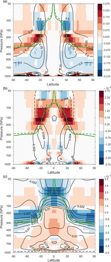
V. A. Sinclair et al.: Extra-tropical cyclones in a warmer climate                                                                    5

Figure 1. Zonal mean (a) temperature (K) and (b) zonal winds (m s−1 ) averaged over 10 years of simulation. Black contours show the CNTL
simulation and shading the difference between the SST4 and control simulations (SST4 − CNTL). The green solid line shows the dynamic
tropopause (the 2 PVU surface) in CNTL and the dashed line in SST4.

cesses can be calculated. Different forms of the omega equa-          Eq. (1). Correlation coefficients between the model calcu-
tion with differing degrees of complexity exist and range             lated vertical motion and the diagnosed vertical motion were
from the simplest “standard” quasi-geostrophic (QG) form              calculated at each grid box and pressure level and averaged
with friction and diabatic heating neglected (Holton and              over latitude bands (not shown). In the latitude band 30–
Hakim, 2012) to the complex generalized omega equation                60◦ N the correlation coefficients were 0.84 at 700 hPa and
(Räisänen, 1995; Rantanen et al., 2017). Here we solve the            exceeded 0.9 at 500 hPa.
following version of the QG omega equation in pressure (p)
coordinates:
                    ∂ 2ω     ∂                                        4   Climatology and large-scale response to warming
σ0 (p)∇ 2 ω + f 2        =f    (v · ∇(ζ + f ))
                    ∂p 2    ∂p
                                                                      In this section the zonal mean climatology of CNTL is de-
                          R                 R 2                       scribed along with the response to the uniform warming. Fig-
                         + ∇ 2 (v · ∇T ) −      ∇ Q.          (1)
                          p                cp p                       ure 1 shows that the control simulation produces a realistic
                                                                      distribution of temperature and of zonal winds. The dynamic
  The static stability parameter, σ0 , is only a function of
                                                                      tropopause varies from 300 hPa in the polar regions to about
pressure and time and is given by
                                                                      100 hPa in the tropics, similar to what is observed on Earth.
           −RT0 1 ∂θ0                                                 The zonal mean jet streams have maximum wind speeds of
σ0 (p) =              ,                                       (2)     45 m s−1 and are located on the tropopause at 35◦ N/S. As
            p θ0 ∂p
                                                                      expected from the aqua-planet model set-up the two hemi-
where θ0 (T0 ) is the horizontally averaged potential tempera-        spheres are almost symmetrically identical.
ture (temperature) profile over the global domain calculated             The response to the uniform 4 K warming is shown by the
at every time step. The left-hand side operator of Eq. (1)            shading in Fig. 1. The temperature increases everywhere in
is identical to the standard QG omega equation. The terms             the troposphere with the largest warming in the tropical up-
on the right-hand side of Eq. (1) represent forcing for ver-          per troposphere, where temperature increases by up to 7 K.
tical motion due to differential vorticity advection, thermal         Cooling takes place in the polar stratosphere, which acts
advection, and diabatic heating. The right-hand side differs          to increase the upper-level meridional temperature gradient.
from the standard QG omega equation in that diabatic heat-            The tropopause height increases at most latitudes with warm-
ing (Q) is retained, the advection terms are calculated us-           ing. The spatial pattern of these changes in zonal mean tem-
ing the full horizontal winds (v) rather than the geostrophic         perature is similar to those found in more complex climate
winds, and the full relative vorticity (ζ ) is advected rather        models (e.g. Fig. 12.12, Collins et al., 2013). However, the
than the geostrophic vorticity. Friction is neglected as on an        warming in the low to mid-troposphere is relatively uniform
aqua planet this is expected to be small.                             with latitude. The lack of enhanced warming in the Northern
   Overall good agreement is found between the model cal-             Hemisphere polar regions (polar amplification) and hence no
culated vertical motion and the vertical motion diagnosed by          decrease in low-level baroclinicity is the most notable differ-

www.weather-clim-dynam.net/1/1/2020/                                                         Weather Clim. Dynam., 1, 1–25, 2020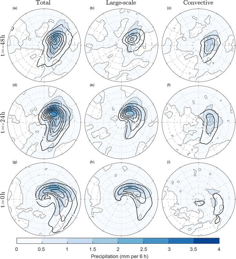
6                                                              V. A. Sinclair et al.: Extra-tropical cyclones in a warmer climate

ence in the atmosphere’s response to warming in these aqua-
planet experiments compared to in complex climate model
simulations.
   At low levels, the increase in temperature in the SST4 ex-
periment relative to CNTL is typically of the order of 4 K,
which is of similar magnitude to the enforced increase in
SSTs. This temperature increase can be put into context by
comparison with predictions from CMIP5 models. Under the
RCP8.5 scenario, CMIP5 models predict that global mean
near-surface temperatures will increase by 2.6 to 4.8 K by
the end of the 21st century relative to the 1986–2005 mean.
Hence, the aqua-planet simulations performed here have a
degree of warming that could be expected to occur by the end
of the 21st century under large greenhouse gas emissions.
   The response of the zonal mean zonal wind shows that
the subtropical jet intensifies and moves vertically upwards.
The eddy-driven jet, evident at low levels, displays a dipole         Figure 2. Zonal mean (a) total precipitation (mm d−1 ), (b) mean
structure indicative of a poleward shift. This is confirmed           sea level pressure (hPa), and (c) 950 hPa temperature (◦ C) averaged
                                                                      over 10 years of simulation. Blue line shows CNTL and red SST4.
when the latitude of the maximum 700 hPa zonal mean zonal
wind speed is considered: this moves polewards by 3.3◦
in the SST4 experiment compared to in CNTL. These re-                 mean 950 hPa temperature, which indicates that the low-level
sponses of the zonal mean jet streams to uniform warming              temperature increase is almost constant with latitude and im-
are similar to those found in more complex climate models             plies that the low-level baroclinicity does not change.
(e.g. Collins et al., 2013), particularly in the Southern Hemi-          The impact of uniformly warming the SSTs on the baro-
sphere, demonstrating that the OpenIFS aqua planet can re-            clinicity can be quantified via the maximum (dry) Eady
alistically simulate an Earth-like atmosphere.                        growth rate, σ , which is given by
   The zonal mean precipitation in both CNTL and SST4 ex-
periments are shown in Fig. 2a. Again strong similarities ex-                    |f | ∂u
ist with real Earth observations and CMIP5 model projec-              σ = 0.31           ,                                            (3)
                                                                                  N ∂z
tions (e.g. Lau et al., 2013). The largest rainfall is observed in
the tropics and a secondary peak occurs in the mid-latitudes,         where f is the Coriolis parameter, N is the Brunt–Väisälä
which is associated with the mid-latitude storm track. The            frequency, and u is the zonal wind component. In the CNTL
effect of warming the SSTs is to increase the mean pre-               simulation (Fig. 3a) the Eady growth rate has maximum val-
cipitation at almost all latitudes. The largest absolute in-          ues of 0.75 day−1 in the mid-latitude middle to upper tro-
crease occurs in the tropics. In the Northern Hemisphere              posphere. A secondary maximum is evident in the strato-
mid-latitudes the maximum precipitation rate increases from           sphere; however, this most likely has little significance for
3.9 to 4.2 mm d−1 and the location of the maximum moves               the growth of extra-tropical cyclones. The response of the
polewards by 2.2◦ . This is in agreement with the poleward            Eady growth rate to warming includes an increase just above
shift in the eddy-driven jet and strongly suggests that, on av-       the dynamical tropopause and a decrease co-located with
erage, extra-tropical cyclones move poleward with warming.            the secondary maximum in the stratosphere. With the mid-
This will be confirmed in Sect. 5.                                    troposphere, the Eady growth rate decreases slightly with
   Figure 2b shows the zonal mean mean sea level pres-                warming; for example, at 700 hPa the maximum value de-
sure (MSLP). The highest zonal mean MSLP in the CNTL                  creases from 0.54 d−1 in CNTL to 0.50 d−1 in SST4. Close
experiment occurs in the subtropics and moves poleward                to the surface, at 900 hPa, the maximum value of the Eady
with warming. The lowest values of MSLP occur on the                  growth rate also experiences a small decrease with warming,
poleward side of the jet stream and again move poleward               from 0.92 to 0.89 d−1 . The most notable impact of warming
with warming. A notable difference between these MSLP                 on the Eady growth rate at 900 hPa is a poleward shift of 5.4◦
distributions and the MSLP distribution on Earth is the ab-           in the position of the maximum. Equatorward of 45◦ N the
solute magnitude of the values. The mean MSLP on Earth is             900 hPa Eady growth rate decreases with warming, whereas
1013 hPa, whereas in both the CNTL and SST4 experiments,              poleward of 45◦ N it increases.
the global mean MSLP is 985.4 hPa. This difference is solely             Figure 3b and c show the vertical shear of the zonal wind
due to the initialization method (see Sect. 2.2), and the aver-       and the Brunt–Väisälä frequency respectively. There is lit-
age surface pressure of 985.4 hPa results, as it is the average       tle change in the vertical wind shear with warming in the
pressure at the actual surface height in the randomly selected        mid-troposphere, which via thermal wind balance is con-
analysis used for the initialization. Figure 2c shows the zonal       sistent with the lack of any large changes to the horizontal

Weather Clim. Dynam., 1, 1–25, 2020                                                       www.weather-clim-dynam.net/1/1/2020/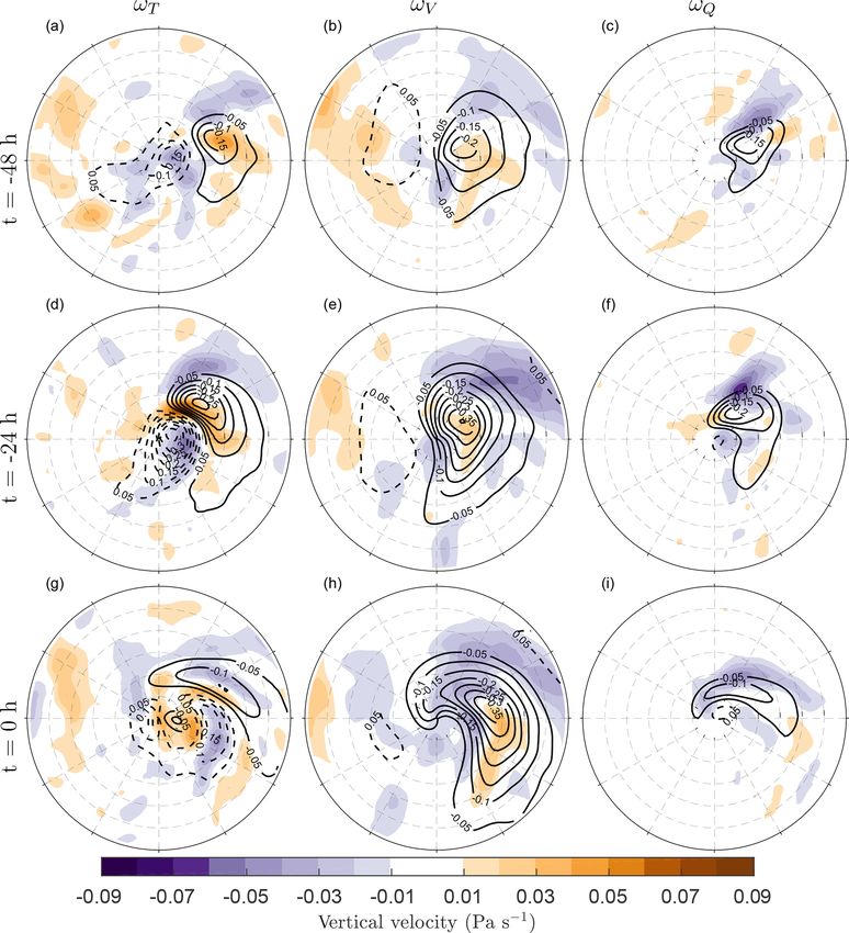
V. A. Sinclair et al.: Extra-tropical cyclones in a warmer climate                                                                  7

                                                                      temperature gradient in the troposphere (Fig. 1a). Near the
                                                                      surface, there is a dipole pattern showing that the maximum
                                                                      in wind shear moves polewards. This is consistent with the
                                                                      poleward shift of the eddy-driven jet and also explains the
                                                                      poleward shift in the 900 hPa Eady growth rates. The Brunt–
                                                                      Väisälä frequency increases in the troposphere, which indi-
                                                                      cates that the decrease in the Eady growth rates at 700 hPa,
                                                                      and at lower latitudes higher up in the troposphere, is due pri-
                                                                      marily to changes in the static stability. Near the tropopause
                                                                      the decrease in the stability associated with an increase in the
                                                                      tropopause height increases the Eady growth rate. In contrast,
                                                                      the decrease in the secondary maximum in the stratosphere
                                                                      is due to changes in the vertical wind shear.

                                                                      5   Cyclone statistics

                                                                      In this section bulk cyclone statistics are presented from
                                                                      both the CNTL and SST4 simulations. All cyclone tracks
                                                                      that meet the criteria described in Sect. 3.1 are included
                                                                      in this analysis, and their mean and median characteristics
                                                                      are summarized in Table 1. In the control simulation there
                                                                      are 3581 extra-tropical cyclones which have a median life-
                                                                      time of 108 h (4.5 d) and a median maximum vorticity of
                                                                      5.94 × 10⁻⁵ s−1 (Table 1). The uniform warming acts to de-
                                                                      crease the total number of cyclone tracks by 3.3 % but does
                                                                      not alter the median duration (lifetime) of extra-tropical cy-
                                                                      clones (Table 1). The inter-annual variability in the number
                                                                      of cyclone tracks, quantified by calculating the number of
                                                                      cyclone tracks each year and then obtaining the standard de-
                                                                      viation of these 10 values, is small (13.5 in CNTL and 10.1 in
                                                                      SST4) relative to the absolute decrease in the number of cy-
                                                                      clone tracks (119). This, and a two-sided Student’s t test,
                                                                      shows that the decrease in the number of tracks is statisti-
                                                                      cally significant.
                                                                         Figure 4a shows histograms of maximum 850 hPa vortic-
                                                                      ity (also referred to hereinafter as maximum intensity). There
                                                                      are more stronger cyclones, for example with intensities ex-
                                                                      ceeding 10 × 10−5 s−1 , in the SST4 experiment than in the
                                                                      CNTL experiment. However, the mean intensity does not
                                                                      change considerably and there is a 3.2 % decrease (equiv-
                                                                      alent to 0.19 × 10⁻⁵ s−1 ) in the median maximum vortic-
                                                                      ity. This change (i.e. the signal) is very small compared to
                                                                      the variation between individual cyclones quantified by the
                                                                      standard deviation of the maximum relative vorticity of all
                                                                      storms (2.55 × 10⁻⁵ s−1 in CNTL). Furthermore, the mean
Figure 3. Zonal mean (a) maximum Eady growth rate (d−1 ),             maximum vorticity for all cyclones occurring in each indi-
(b) vertical shear of the zonal wind (s−1 ), and (c) Brunt–Väisälä    vidual year can be obtained and the standard deviation of
frequency (s−1 ) averaged over 10 years of simulation. Black con-     these 10 values calculated to obtain the inter-annual stan-
tours show the CNTL simulation, and shading shows the difference      dard deviation of the maximum relative vorticity. For CNTL
between the SST4 and control simulations (SST4 − CNTL). In (c)        this is 0.14 × 10⁻⁵ and 0.10 × 10⁻⁵ s−1 in SST4, which are
contours are every 0.002 s−1 for values greater than 0.01 s−1 , and   both larger than the absolute change in the mean maximum
the dashed line shows the 0.005 s−1 contour. The green solid line
                                                                      relative vorticity (−0.04 × 10⁻⁵ s−1 , Table 1). A two-sided
shows the dynamic tropopause (the 2 PVU surface) in CNTL and
                                                                      Student’s t test further confirms that the mean intensity does
the green dashed line in SST4.
                                                                      not differ in a statistically significant way between CNTL

www.weather-clim-dynam.net/1/1/2020/                                                       Weather Clim. Dynam., 1, 1–25, 2020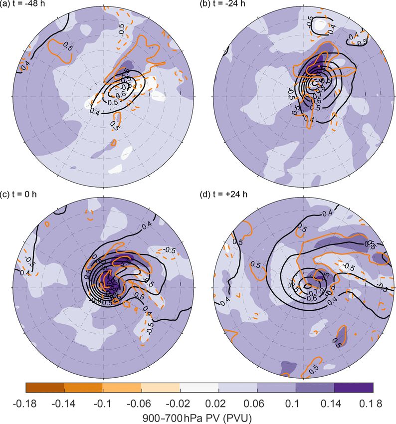
8                                                              V. A. Sinclair et al.: Extra-tropical cyclones in a warmer climate

Figure 4. Normalized histograms of the extra-tropical cyclone’s (a) maximum 850 hPa relative vorticity, (b) average deepening rate between
time of genesis and time of maximum vorticity, (c) genesis latitude, and (d) lysis latitude. Blue shows CNTL and red shows SST4.

and SST4, and a Wilcoxon rank-sum test shows that the me-              between the time of genesis and time of maximum intensity
dian maximum intensities are not statistically significantly           confirms that the median values are not statistically different.
different between the CNTL and SST4 experiments. How-                  The same test applied to the deepening rates calculated over
ever, as evident from Fig. 4a, and confirmed by a one-tailed           the 24 h before the time of maximum intensity also shows
F test applied to the maximum vorticity distributions, the             that the control and SST4 experiments do not differ signifi-
maximum vorticity distribution in the SST4 experiment has              cantly. However, similar to what is found with the maximum
a larger variance than in the CNTL experiment. Thus, it can            vorticity distributions, the variance of the deepening rates
be concluded that the average population of all cyclones does          is statistically significantly larger in the SST4 experiment
not change with warming but that there are more stronger and           compared to in CNTL. The lack of any notable change in
more weak cyclones in the SST4 experiment than in CNTL.                the median deepening rate of all extra-tropical cyclones dif-
   Table 1 also includes the median deepening rates of all             fers somewhat from the zonal mean calculations of the Eady
extra-tropical cyclones. The deepening rate is the temporal            growth rate (Fig. 3a), which indicate a 5 %–10 % decrease.
rate of change of the 850 hPa relative vorticity so that positive      This difference likely arises because the Eady growth rate is
values indicate a strengthening, or deepening, of the extra-           a measure of dry baroclinicity whereas moist processes are
tropical cyclone. In CNTL, the relative vorticity increases            acting in these simulations.
by 1.31 × 10⁻⁵ s−1 every 24 h when evaluated from genesis                 Distributions of the genesis and lysis latitudes for all extra-
time to time of maximum intensity. In SST4, the correspond-            tropical cyclones are shown in Fig. 4c and d. As hypothesized
ing value is 1.28 × 10⁻⁵ s−1 per 24 h. The change is very              in Sect. 4, both genesis and lysis regions move poleward with
small in comparison to the standard deviation of the deep-             warming. The median genesis region moves 2◦ polewards
ening rates (Table 1). Distributions of the deepening rates of         from 44.2 to 46.2◦ N, and the median lysis region moves
all identified extra-tropical cyclones calculated between the          poleward by 1.9◦ from 51.4 to 53.3◦ N (Table 1). The inter-
time of genesis and time of maximum intensity are shown in             annual standard deviation of the genesis latitude is 0.27◦ in
Fig. 4b. A rank-sum test performed on the deepening rates              CNTL and 0.69◦ in SST4, suggesting that the 2◦ poleward

Weather Clim. Dynam., 1, 1–25, 2020                                                        www.weather-clim-dynam.net/1/1/2020/
V. A. Sinclair et al.: Extra-tropical cyclones in a warmer climate                                                                          9

Table 1. Cyclone statistics from CNTL and SST4. Relative vorticity values have units of ×10−5 s−1 . Duration (lifetime) is given in units of
hours. Deepening rates (units of ×10−5 s−1 (24 h)−1 ) are the temporal rate of change of the 850 hPa relative vorticity. Positive deepening
rate values indicate a strengthening, or deepening, of the extra-tropical cyclone. For vorticity, duration, and deepening rates, change is the
relative change ((SST4 − CNTL)/CNTL) given as a percentage. For genesis and lysis latitude, change is the absolute change.

                                                                               All cyclones                    Strongest 200 cyclones
  Diagnostic                                                        CNTL        SST4          Change      CNTL        SST4       Change
  Number of tracks/cyclones                                         3581        3462          −3.3 %      200         200        0%
  Mean maximum 850 hPa vorticity                                    6.11        6.07          −0.7 %      11.55       11.87      +2.8 %
  Median maximum 850 hPa vorticity                                  5.94        5.75          −3.2 %      11.24       11.56      +2.8 %
  Standard deviation of maximum 850 hPa vorticity                   2.55        2.80          +9.8 %      1.00        1.22       +22 %
  Mean track duration                                               132.3       127.8         −3.4 %      209.7       190.8      −9.9 %
  Median track duration                                             108.0       108.1         0%          192.0       180.0      −6.25 %
  Standard deviation of track duration                              77.3        73.5          −4.9 %      83.0        83.2       +0.24 %
  Median deepening rate (genesis to t = 0 h)                        1.31        1.28          −2.3 %      2.63        3.36       +27.7 %
  Standard deviation of deepening rate (genesis to t = 0 h)         1.13        1.25          +10.6 %     1.43        1.65       +15.4 %
  Median deepening rate (−24 h to t = 0 h)                          1.42        1.43          +0.7 %      3.57        4.41       +23.5 %
  Standard deviation of deepening rate (−24 h to t = 0 h)           1.25        1.42          +13.6 %     1.53        1.75       +14.37 %
  Median genesis latitude                                           44.2◦ N     46.2◦ N       +2.0◦       37.8◦ N     38.2◦ N    +0.4◦
  Median lysis latitude                                             51.4◦ N     53.3◦ N       +1.9◦       51.2◦ N     55.0◦ N    +3.8◦
  Standard deviation of genesis latitude                            12.8◦       13.7◦         +0.9◦       8.6◦        8.9◦       +0.3◦
  Standard deviation of lysis latitude                              13.8◦       14.7◦         +0.9◦       11.3◦       11.0◦      −0.3◦
  Median dlat (lysis–genesis latitude)                              6.2◦        6.0◦          −0.2◦       13.7◦       16.7◦      +3.0◦
  Median dlat (max vort lat–genesis latitude)                       2.9◦        2.9◦          0◦          9.0◦        9.3◦       +0.3◦
  850 hPa relative vorticity threshold for strongest 200 cyclones   –           –             –           10.44       10.88      +4.2 %
  Vorticity of the strongest cyclone                                –           –             –           15.55       16.80      +8.1 %
  Maximum deepening (genesis to time of max)                        –           –             –           7.05        9.10       +29.0 %

shift in genesis latitude is significant. Likewise, the inter-           the median genesis latitude of the 200 strongest extra-tropical
annual standard deviation of the lysis latitude is 0.52 and              cyclones only moves 0.4◦ poleward with warming, which
0.72◦ in CNTL and SST4 respectively and therefore also                   is notably less than the 2.0◦ poleward shift found when all
smaller than the response to warming. Two-sided Student’s                extra-tropical cyclones are considered. Thirdly, deepening
t tests show that the mean genesis latitude differs between the          rates increase much more with warming for the strongest
CNTL and SST4 experiments at the 95 % confidence level                   200 extra-tropical cyclones than for all extra-tropical cy-
and that both the median genesis and lysis latitudes differ              clones. Finally, the mean, median, and maximum intensity
significantly at the 0.05 significance level. The standard de-           of the 200 strongest extra-tropical cyclones in the SST4 ex-
viation of both the genesis latitude (12.8◦ in CNTL, Table 1)            periment are larger than in the CNTL experiment.
and lysis latitude (13.7◦ in CNTL, Table 1) of all cyclones
is larger than the mean change in genesis and lysis latitudes,
indicating that the change is small compared to the variation            6     Cyclone structure
between individual cyclones.
   Table 1 also includes statistics for the strongest 200 extra-         6.1     Evolution of the composite cyclone in CNTL
tropical cyclones in each experiment as the structure of these
intense extra-tropical cyclones will be investigated in de-              The cyclone composite of the strongest 200 extra-tropical cy-
tail in Sect. 6. Firstly, the median genesis latitudes of the            clones in the CNTL experiment is now discussed. The tem-
strongest extra-tropical cyclones are 6 to 8◦ farther equator-           poral evolution of the composite mean cyclone in the CNTL
ward than for all extra-tropical cyclones in both the CNTL               simulation, in terms of mean sea level pressure and total
and SST4 experiments, which means that the strongest                     column water vapour (TCWV) is shown in Fig. 5. A total
storms form in climatologically warmer and more moist en-                of 48 h before the time of maximum intensity (t = −48 h,
vironments than average-intensity storms. The more equa-                 Fig. 5a) the composite cyclone has a closed low-pressure
torward genesis region, combined with similar (CNTL) or                  centre with a minimum MSLP of 978 hPa. The location of
more poleward (SST4) lysis regions, means that the strongest             the cold and warm fronts is evident as enhanced gradients in
extra-tropical cyclones have much larger latitudinal displace-           the TCWV and the warm sector, located between the cold
ments than extra-tropical cyclones do on average. Secondly,              front and warm front, are well defined and have values of

www.weather-clim-dynam.net/1/1/2020/                                                              Weather Clim. Dynam., 1, 1–25, 2020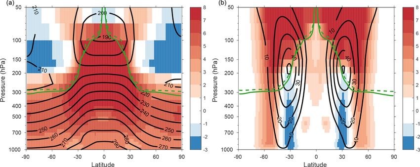
10 V. A. Sinclair et al.: Extra-tropical cyclones in a warmer climate
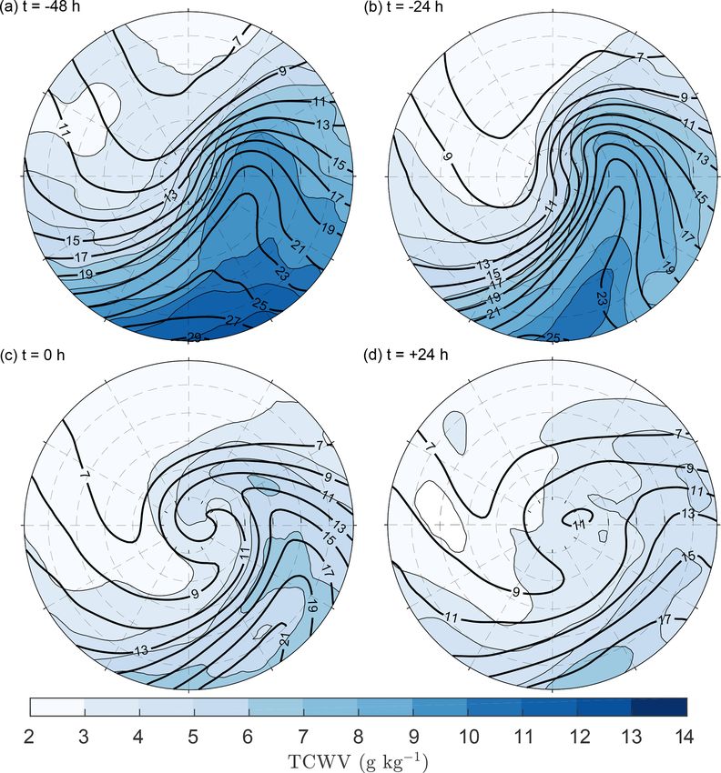
Figure 5. Composite cyclone of the strongest 200 extra-tropical cyclones in the CNTL simulation at (a) 48 h before time of maximum
vorticity, (b) 24 h before time of maximum vorticity, (c) time of maximum vorticity, and (d) 24 h after the time of maximum vorticity.
Shading shows the total column water vapour (g kg−1 ), and black contours show the mean sea level pressure (hPa). The plotted radius is 12◦ .
TCWV exceeding 25 g kg−1 . At 24 h before the time of max- after the time of maximum intensity (t = +24 h, Fig. 5d), the
imum intensity (t = −24 h, Fig. 5b) the low-pressure centre cyclone resembles a barotropic low and has weak frontal gra-
has become deeper (minimum MSLP of 960 hPa), the warm dients associated with it. The evolution of the composite cy-
sector has become narrow and the gradients in TCWV across clone in the CNTL experiment is, however, qualitatively very
both the warm and cold fronts have become larger. The dry similar to real extra-tropical cyclones observed on Earth.
air moving cyclonically behind the cold front now extends
farther south relative to the cyclone centre than it did 24 h 6.2 Low-level potential and relative vorticity
earlier. By the time of maximum relative vorticity (t = 0 h,
Fig. 5c), the MSLP shows a mature, very deep cyclone which The response of the cyclone structure to warming is now
has a minimum pressure of 944 hPa. The TCWV over the considered primarily using changes to the mean values
whole cyclone composite area is now considerably lower (i.e. SST4 − CNTL). First the temporal evolution of the low-
than at earlier stages most likely because as the cyclones in- level potential vorticity (PV) and the changes to this variable
cluded in the composite intensify they move poleward to cli- with warming are considered (Fig. 6). Before the compos-
matologically drier areas. The TCWV pattern also shows that ite cyclone reaches it maximum intensity (Fig. 6a and b), the
the composite cyclone starts to occlude by this point (t = 0 h) maximum in the 900–700 hPa layer-averaged PV in the con-
as the warm sector does not connect directly to the centre of trol simulation is poleward and downstream of the cyclone
the cyclone – instead it is displaced downstream. Finally 24 h centre. By the time of maximum intensity (Fig. 6c), the max-
imum PV is co-located with the cyclone centre and there is
Weather Clim. Dynam., 1, 1–25, 2020 www.weather-clim-dynam.net/1/1/2020/V. A. Sinclair et al.: Extra-tropical cyclones in a warmer climate 11 Figure 6. Composite mean of the strongest 200 extra-tropical cyclones at (a) 48 h before time of maximum vorticity, (b) 24 h before time of maximum vorticity, (c) time of maximum vorticity, and (d) 24 h after the time of maximum vorticity. Black contours show the 900–700 hPa layer mean potential vorticity in CNTL (contour interval 0.1 PVU, starting at 0.4 PVU). Shading shows the difference in the 900–700 hPa layer mean potential vorticity between SST4 and CNTL. Orange contours show the difference in the 850 hPa relative vorticity between SST4 and CNTL (contour interval 0.5 × 10⁻⁵ s−1 , the 0 contour is omitted). Solid orange contours show positive differences and dashed contours negative differences. a secondary maximum which extends downstream of the cy- front, as found at the earlier stages of development, and the clone centre and is co-located with the warm front. second is almost co-located with the cyclone centre yet dis- At t = −48 and t = −24 h, the largest absolute increases placed slightly downstream. Both localized increases in low- in the 900–700 hPa PV occur poleward of the warm front level PV are also associated with increases in relative vortic- location (Fig. 6a and b). This low-level PV anomaly is pri- ity. In relative terms (not shown) the low-level potential vor- marily caused by a diabatic heating maximum above this ticity poleward of the warm front increases by 25 %–30 %, layer and therefore the poleward movement of the maxi- whereas near the cyclone centre the low-level PV only in- mum indicates that the maximum in diabatic heating has also creases by 15 %–20 %. moved polewards with warming. The increase in PV is co- The response to warming also shows that almost every- located with an increase in relative vorticity (orange con- where within a 12◦ radius of the cyclone centre, at all offset tours in Fig. 6), which is consistent with an intensified cy- times, there is an increase in low-level PV. The absolute val- clonic circulation beneath a region of localized heating. It ues of increase are smaller, mostly less than 0.1 PVU, but can therefore be concluded that the relative vorticity associ- in relative terms the increase is similar in magnitude to that ated the warm front increases with warming. At t = 0 and found near the warm front and cyclone centre. Away from t = +24 h (Fig. 6c and d), two distinct regions of increased the cyclone centre, where there is no significant relative vor- low-level PV are evident. The first is poleward of the warm ticity, this increase in low-level PV is primarily caused by an www.weather-clim-dynam.net/1/1/2020/ Weather Clim. Dynam., 1, 1–25, 2020
12 V. A. Sinclair et al.: Extra-tropical cyclones in a warmer climate
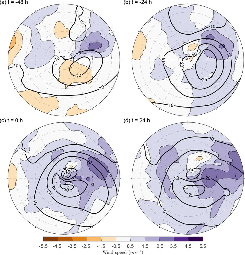
Figure 7. Composite mean of the 900 hPa wind speed of the strongest 200 extra-tropical cyclones in the CNTL simulation (black contours,
every 5 m s−1 ) and the difference between SST4 and CNTL (shading) at (a) 48 h before time of maximum intensity, (b) 24 h before time of
maximum intensity, (c) time of maximum intensity, and (d) 24 h after the time of maximum intensity.
increase in stratification. However, given that the cyclones (Fig. 7a). However, the positive values are greater in magni-
are more poleward in the SST4 experiment, the increase in tude than the negative values, thus indicating an overall in-
planetary vorticity also plays a small role. crease in wind speed. At t = −24, 0, and 24 h (Fig. 7b–d)
the 900 hPa winds speeds of the composite cyclone increase
6.3 Low-level wind speed with warming by ∼ 1.5 m s−1 in a large area surrounding the
cyclone and by up to 3.5 m s−1 in the warm front area. Con-
Figure 6 highlights that the relative vorticity increases with sequently, the size of the area affected by wind speeds over a
warming at all offset times. Associated with this increase fixed threshold value increases, indicating greater wind risk
in relative vorticity is an increase in low-level horizontal in warmer climates. As the increase at all offset times is not
wind speeds. In the composite from the CNTL experiment, at co-located with maximum wind speed in CNTL, this sug-
t = −48 and t = −24 h (Fig. 7a and b), the strongest 900 hPa gests that the spatial structure of the composite extra-tropical
wind speeds exceed 20 and 25 m s−1 respectively and oc- cyclone changes with warming.
cur in the warm sector. At the time of maximum intensity
(Fig. 7c), the strongest 900 hPa winds in CNTL are located 6.4 Total column water vapour
equatorward of the cyclone centre, behind the cold front in a
very dry area, and exceed 30 m s−1 . By t = 24 h (Fig. 7d) The response of the TCWV is now considered (Fig. 8). The
the wind speeds have started to weaken. At t = −48 h, a uniform warming leads to an increase in TCWV everywhere
dipole structure in the change in wind speed due to warm- in the cyclone composite at all offset times. The largest ab-
ing is evident, indicating that the maximum wind speeds solute increases occur at t = −48 and t = −24 h (Fig. 8a
move poleward and downstream relative to those in CNTL and b). At both of these offset times, the largest absolute in-
Weather Clim. Dynam., 1, 1–25, 2020 www.weather-clim-dynam.net/1/1/2020/V. A. Sinclair et al.: Extra-tropical cyclones in a warmer climate 13
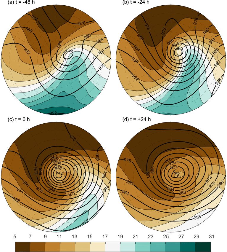
Figure 8. Composite mean of the total column water vapour (TCWV) of the strongest 200 extra-tropical cyclones in the CNTL simulation
(black contours, every 2 g kg−1 ) and the difference between SST4 and CNTL (shading) at (a) 48 h before time of maximum intensity, (b) 24 h
before time of maximum intensity, (c) time of maximum intensity, and (d) 24 h after the time of maximum intensity.
crease occurs in the warm sector where the mean values are 6.5 Precipitation
largest in the control simulation. In terms of percentage in-
crease (not shown), at t = −24 h, the TCWV increases the The response of the total, convective, and large-scale precip-
least, approximately 25 %, in the cold sector upstream of the itation to warming is now considered. Composites of total,
cyclone centre and the most ahead of the warm front where large-scale, and convective precipitation are shown in Fig. 9
the increase exceeds 50 %. At the time of maximum intensity valid 48, 24, and 0 h before the time of maximum intensity.
(Fig. 8c), absolute increases of up to 6 g kg−1 are still evi- Precipitation is calculated as the 6 h accumulated value cen-
dent in the warm sector and in a localized region northeast of tred on the valid time in units of millimetres per 6 h. In the
the cyclone centre, whereas at t = +24 h (Fig. 8d) increases CNTL simulation the maximum total precipitation is down-
of this magnitude are constrained to the most southern part stream and poleward of the cyclone centre at all offset times.
of the cyclone composite. The composites also show the At t = −48 h, the total precipitation has maximum values of
meridional moisture gradient across the composite cyclone 6 mm (6 h)−1 and is mainly located in the warm sector of the
increases notably with warming since the absolute increase is cyclone and near the warm front (Fig. 9a). At t = −24 h, the
much larger in the most equatorward regions (e.g. 12 g kg−1 total precipitation in the CNTL simulation is slightly larger,
at t = −48 h) than in the most poleward regions (e.g. an in- covers a greater area, and has a more distinct comma shape
crease of 2 g kg−1 ). than 24 h earlier (Fig. 9d). Also at this time, large values of
total precipitation are evident along the cold front to the south
of the cyclone centre. By the time of maximum intensity the
total precipitation in the CNTL experiment has started to de-
www.weather-clim-dynam.net/1/1/2020/ Weather Clim. Dynam., 1, 1–25, 202014 V. A. Sinclair et al.: Extra-tropical cyclones in a warmer climate Figure 9. Composites of total precipitation (a, d, g), large-scale precipitation (b, e, h), and convective precipitation (c, f, i) in the CNTL simulation (black contours) and the difference between SST4 and control (shading). Panels (a)–(c) are valid 48 h before the time of maximum intensity, panels (d)–(f) are valid 24 h before the time of maximum intensity, and panels (g)–(i) are valid at the time of maximum intensity. All composites are of the strongest 200 extra-tropical cyclones in each experiment. crease, with maximum values of 4 mm (6 h)−1 , and the loca- 2.0 mm (6 h)−1 at t = −48, t = −24 h, and the time of max- tion of the precipitation has rotated cyclonically around the imum vorticity (t = 0 h) respectively. These values corre- cyclone centre (Fig. 9g). spond to relative increases of up to almost 50 %. The maxi- The response to warming of the total precipitation is a mum increase in the total precipitation is not co-located with large absolute and relative increase at all offset times. The the maximum in the CNTL simulation, indicating that the maximum absolute increases are of the order of 2.5, 3.5, and spatial structure of the composite cyclone has changed with Weather Clim. Dynam., 1, 1–25, 2020 www.weather-clim-dynam.net/1/1/2020/
V. A. Sinclair et al.: Extra-tropical cyclones in a warmer climate 15
warming. The largest increases in total precipitation occur in Fig. 10a, c, and e. In the CNTL simulation at t = −48 and
in the warm front region, poleward and downstream of the t = −24 h, there is large coherent area of ascent downstream
maximum in the CNTL simulation at all offset times. This of the cyclone centre largely co-located with the warm sector
spatial change is largely similar to that found when the 900– indicative of the warm conveyor belt, an ascending airstream
700 hPa potential vorticity response to warming was consid- associated with extra-tropical cyclones. At t = 0 h (Fig. 10e),
ered (Fig. 6). This is consistent in the sense that more precipi- the area of ascent is still maximized in the warm sector region
tation, and particularly more condensation, results in more la- but is further downstream relative to the cyclone centre than
tent heating and thus a stronger positive PV anomaly beneath at earlier times. The ascent at t = 0 h has also started to wrap
the localized heating. However at t = 0 h, it is interesting to cyclonically around the poleward and upstream side of the
note that while there is only one localized area where pre- cyclone, meaning that the cyclone has formed a bent-back
cipitation increases in SST4 compared to in CNTL (Fig. 9g), warm front and likely has started to occlude. The absolute
which is ahead of the warm front, there are two regions where magnitude of the largest values of ascent occur at t = −24 h
the low-level PV increases (Fig. 6c). One of these regions is and exceed 0.6 Pa s−1 (Fig. 10c), approximately 6 cm s−1 . A
co-located with the increase in precipitation but the second region of weak descent is evident behind the cold front in the
region is closer to the cyclone centre. While this may be due drier air mass at all offset times.
to the larger mean relative vorticity of the strongest 200 cy- Uniform warming changes the vertical motion in a com-
clones in SST4 compared to CNTL (Table 1), it is also pos- plex manner. The largest increases in ascent are not co-
sible that this second area of enhanced PV may be due to en- located with the strongest ascent in the CNTL simulation and
hanced advection by the cold conveyor belt of PV produced instead occur poleward and downstream of the maximum.
diabatically in the warm front region, beneath the ascending This pattern is present at all offset times and suggests that
warm conveyor belt. Schemm and Wernli (2014) noted such the warm front and the warm conveyor belt are located far-
a mechanism in their study linking warm and cold conveyor ther poleward relative to the cyclone centre in the SST4 sim-
belts. ulation. This is consistent with the response of the total and
The contribution of the large-scale stratiform precipitation large-scale precipitation, and the low-level potential vortic-
calculated from the cloud scheme and the convective precipi- ity, which also showed a poleward shift in the warm frontal
tation produced by the convection scheme to the total precip- region. A tri-pole structure is also evident in Fig. 10a, c,
itation is now considered. In CNTL, the large-scale precip- and e, which show that the area of ascent either weakens in
itation (Fig. 9b, e, and h) contributes more to the total pre- the centre and broadens with warming or the ascent associ-
cipitation than the convective precipitation (Fig. 9c, f, and i), ated with the warm and cold fronts becomes more spatially
particularly at t = −24 h and the time of maximum inten- separate with warming. The first of these two options will
sity. However, the convective precipitation is larger and of prove to be correct.
equal magnitude to the large-scale precipitation in the more To further understand the spatial pattern of the response
equatorward parts of the warm sector of the CNTL compos- of the vertical velocity to warming, the contribution to the
ite cyclone where the temperature and moisture content are total vertical velocity from vorticity advection, thermal ad-
higher. The large-scale precipitation increases in SST4 com- vection, and diabatic processes as diagnosed by the omega
pared to CNTL in the warm frontal region, poleward of the equation (Eq. 1) is examined. The sum of these three terms
maximum in the CNTL simulation, at all offset times. This (Fig. 10b, d, and f) at 700 hPa is first compared to the to-
spatial shift is very similar to that observed for the total pre- tal model calculated vertical motion (Fig. 10a, c, and e). At
cipitation, meaning that the resolved precipitation is leading t = −48 h, the diagnosed ascent in CNTL is slightly weaker
to the poleward shift in the total precipitation with warming. than the model-calculated (i.e. direct from OpenIFS) ascent,
However, the large-scale precipitation also has a smaller in- particularly in the cold front region. The response of the
crease (1–1.5 mm per 6 h) in a narrow band along the cold diagnosed vertical motion to warming is however spatially
front, upstream of the maximum in the control simulation, similar to that of the model-calculated vertical motion. At
which is most evident at t = −24 h. In contrast, the convec- t = −24 h, the diagnosed ascent is slightly stronger than the
tive precipitation, which increases by almost 50 %, has the model-calculated ascent and covers a larger area, especially
largest increases co-located with the maximum in the control in the zonal direction. In addition, the descent diagnosed
simulation, meaning that the position of convective precip- from Eq. (1) covers a smaller area than descent in the model-
itation relative to the cyclone centre does not change with calculated vertical motion field. Similar differences between
warming. the model-calculated and diagnosed vertical motion occur
at t = 0 h. There is, however, broad agreement between the
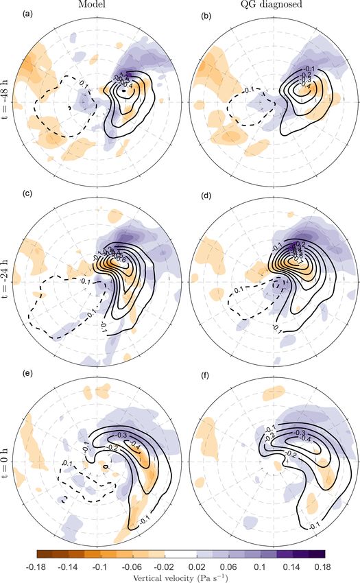
6.6 Vertical velocity model-calculated vertical motion and the vertical motion di-
agnosed using Eq. (1) in CNTL at all offset times, and the
The mean cyclone composite of vertical velocity at 700 hPa response to warming in the diagnosed vertical motion field is
(given in pressure coordinates, Pa s−1 ) obtained directly from very similar to that in the model-calculated field. Thus, the
the model simulations and the response to warming is shown individual contributions to the diagnosed ascent will provide
www.weather-clim-dynam.net/1/1/2020/ Weather Clim. Dynam., 1, 1–25, 2020You can also read