A Search for Mountain Waves in MLS Stratospheric Limb Radiances from the Winter Northern Hemisphere: Data Analysis and Global Mountain Wave Modeling
←
→
Page content transcription
If your browser does not render page correctly, please read the page content below
A Search for Mountain Waves in MLS Stratospheric
Limb Radiances from the Winter Northern Hemisphere:
Data Analysis and Global Mountain Wave Modeling

Jonathan H. Jiang1, Stephen D. Eckermann2, Dong L. Wu1, and Jun Ma3

1
    Jet Propulsion Laboratory, California Institute of Technology, Pasadena, California, USA
2
    Middle Atmosphere Dynamics Section, Naval Research Laboratory, Washington, DC., USA
3
    Computational Physics, Inc., Springfield, Virginia 22151, USA

    J. G. R. – Atmospheres:             In Press

    Short title: Mountain waves in the northern winter stratosphere

    Key Words:
    Gravity waves, dynamics, general circulation, global modeling, vortex, jet-stream, remote sensing, and
    climate

                                                                                                             1
Abstract

   Despite evidence from ground-based data that flow over mountains is a dominant
source of gravity waves (GWs) for the Northern Hemisphere winter middle atmosphere,
GW-related signals in global limb radiances from the Microwave Limb Sounder (MLS)
on the Upper Atmosphere Research Satellite (UARS) have shown little direct evidence of
mountain waves. We address this issue by combining a renewed analysis of MLS limb-
track and limb-scan radiances with global mountain wave modeling with the Naval
Research Laboratory Mountain Wave Forecast Model (MWFM). MLS radiance variances
show characteristics consistent with mountain waves, such as enhanced variance over
specific mountain ranges and annual variations that peak strongly in winter. However,
direct comparisons of MLS variance maps with MWFM-simulated mountain wave
climatologies reveal limited agreement. We develop a detailed “MLS GW visibility
function” that accurately specifies the three-dimensional in-orbit sensitivity of the MLS
limb-track radiance measurement to a spectrum of GWs with different wavelengths and
horizontal propagation directions. On post-processing MWFM-generated mountain wave
fields through these MLS visibility filters, we generate MWFM variance maps that agree
substantially better with MLS radiance variances. This combined data analysis and MLS-
filtered MWFM modeling leads us to conclude that many MLS variance enhancements
can be associated with mountain waves forced by flow over specific mountainous terrain.
These include mountain ranges in Europe (e.g., Scandinavia; Alps; Scotland; Ural,
Putoran, Altai, Hangay and Sayan Mountains; Yablonovyy, Stanovoy, Khingan,
Verkhoyansk and Central Ranges), North America (e.g., Brooks Range, MacKenzie
Mountains, Colorado Rockies), southeastern Greenland and Iceland. Our results show
that, given careful consideration of the in-orbit sensitivity of the instrument to GWs,
middle atmospheric limb radiances measured from UARS MLS, as well as from the new
MLS instrument on the Earth Observing System (EOS) satellite, can provide important
global information on mountain waves in the extratropical Northern Hemisphere
stratosphere and mesosphere.

                                                                                        2
1. Introduction

   Atmospheric gravity waves (GWs) play crucial roles in driving the general circulation

and thermal structure of the atmosphere. Quasi-continuous GW breaking at a range of

heights around the globe maintains body forces and turbulent diffusion that drive winds,

temperatures and chemical constituent distributions well away from those of an

atmosphere lacking these processes [e.g,, Andrews, 1987; Holton and Alexander, 2000;

McIntyre, 2001; Fritts and Alexander, 2003]. Since the spectrum of breaking gravity

waves is not resolved in global climate and weather prediction models at present, these

unresolved GW processes must be comprehensively parameterized so that models can

reproduce realistic circulations on both short and long time scales [see, e.g., Hamilton,

1996; McLandress, 1998; Kim et al., 2003]. Gravity waves can produce other important

effects, such as wave clouds at various heights that can have important follow-on effects

on processes such as precipitation and ozone [e.g., Jensen and Toon, 1994; Carslaw et

al., 1998; Koch and Siedlarz, 1999; Thayer et al., 2003]. This has led to a new class of

parameterizations of subgridscale gravity wave effects on clouds for global models [e.g.,

Cusack et al., 1999; Bacmeister et al., 1999; Pierce et al., 2003].

   GWs are generated by a variety of processes in the lower atmosphere [Fritts and

Alexander, 2003]. Of these, flow over mountains is believed to be one of the dominant

sources, particularly in the extratropics during winter [e.g., Nastrom and Fritts, 1992].

The drag produced by the breaking of these so-called mountain waves is important for

both short-term weather prediction and long-term climate modeling, and so considerable

effort has been devoted to mountain wave drag parameterization schemes for global

models [see, e.g., Kim et al., 2003].

                                                                                       3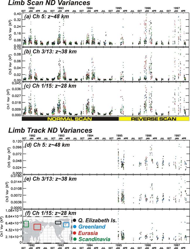
Unfortunately, many aspects of GW parameterizations are uncertain and highly

simplified, due mainly to a lack of detailed global data on GWs which could be used to

intercompare, assess and constrain the various models of these processes currently in use.

This paucity of global data has arisen because, until recently, limb and nadir viewing

remote-sensing instruments on satellites lacked the spatial or temporal resolution to

resolve atmospheric GW perturbations. Fetzer and Gille [1994], however, showed that

raw temperature data acquired by the Limb Infrared Monitor of the Stratosphere (LIMS)

on the Nimbus-7 satellite resolved long wavelength gravity wave fluctuations. During the

last decade, other high-resolution satellite instruments have attained the necessary

resolutions and accuracies to provide our first tentative global glimpses of these long

wavelength portions of the GW spectrum. One of the most important instruments in this

critical emerging database has been the Microwave Limb Sounder (MLS) on the Upper

Atmosphere Research Satellite (UARS) [Waters et al., 1999]. Since the mid-1990’s,

UARS MLS 63 GHz radiance fluctuations have been used to study global GW

morphologies in the stratosphere and mesosphere [Wu and Waters, 1996a,b; Wu and

Waters, 1997; Alexander, 1998; McLandress et al., 2000; Wu, 2001; Jiang and Wu, 2001;

Wu and Jiang, 2002; Jiang et al., 2002; Jiang et al., 2003a,b].

   Previous global maps of MLS radiance variances in the stratosphere and mesosphere

showed good correlations between enhanced variance and strong background wind

speeds [e.g. Wu and Waters, 1996a,b; Wu and Waters, 1997; McLandress et al., 2000;

Jiang and Wu, 2001]. Alexander [1998] showed that much of this structure could be

reproduced by a simple source-independent GW ray-tracing model, which accounted for

the Doppler-shifting effects of background winds on the gravity wave spectrum and the

finite vertical width of the MLS channel weighting functions, which allowed only those

                                                                                         4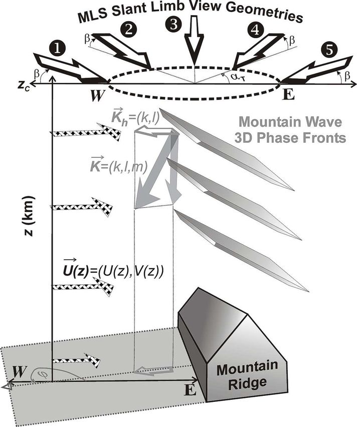
waves with long vertical wavelengths to be resolved. McLandress et al. [2000] performed

a detailed follow-up study of MLS variances measured by channels 3 and 13 (altitudes

z~38 km) and used a similar global GW ray model to simulate the observed variance

distributions. Their work showed that refraction and observational filtering of waves by

background winds alone could not explain all of the structure in MLS GW variance

maps. For example, model sensitivity experiments suggested that large increases in

stratospheric variances in the summer subtropics and in winter over the southern Andes

were consistent with intense local generation of gravity waves from underlying

convective and topographic sources, respectively.

   Eckermann and Preusse [1999] analyzed a week’s worth of infrared limb temperature

data acquired by the CRISTA instrument on the Shuttle Pallet Satellite in November,

1994. After isolating stratospheric temperature perturbations, they used simple theory and

output from the Naval Research Laboratory (NRL) Mountain Wave Forecast Model

(MWFM) to show that enhanced stratospheric temperature fluctuations over the southern

tip of South America were produced by mountain waves forced by flow across the

Andes. A detailed follow-up study by Preusse et al. [2002] confirmed this using retrieval

modeling, GW theory, a mesoscale model and ray-tracing experiments. Given these

indications, Jiang et al. [2002] conducted a thorough study of stratospheric radiance

variances over the southern Andes region, utilizing slightly more than 2 years of MLS

limb track data between late 1994 and early 1997. Variances over the Andes exhibited a

strong annual variation, peaking in winter, with somewhat weaker wintertime activity in

1996 compared to 1995. These features were reproduced quite well by a detailed MWFM

“hindcast” simulation formulated for this particular time period. Wu and Jiang [2002]

                                                                                        5
also reported enhancements of MLS variances over Antarctica that may also be mountain

wave-related.

   Mountain waves are believed to be more energetic and geographically prevalent in

the Northern Hemisphere [Bacmeister, 1993; Fritts and Alexander, 2003], due to the

more extended mountainous landmasses in this hemisphere. Yet little if any progress has

been made to date in extracting unambiguous data on mountain waves from MLS

radiances in the Northern Hemisphere. McLandress et al. [2000] documented highly

structured variance distributions in the northern extratropics, but they were unable to

draw conclusions as to the sources of this wave activity because strong longitudinal and

day-to-day variations in stratospheric wind fields complicated their model-data

comparisons. Jiang and Wu [2001] further demonstrated how strong variable

stratospheric flow fields in the north substantially modulated MLS variances, seemingly

masking any signatures of wave sources. Such difficulties do not appear to be unique to

MLS. Despite showing clear evidence of enhanced stratospheric temperature variance

from gravity waves over deep tropical convection, GPS/MET occultation data have to

date yielded little clear evidence of enhanced temperature variances over mountains in

the Northern Hemisphere during winter [Tsuda et al., 2000].

   Despite these complications, MLS satellite data do show occasional hints of variance

enhancements over topography during northern winter. For example, Figure 5b of

McLandress et al. [2000] shows enhancements in limb track variances over mountainous

regions such as Scandinavia, central Eurasia, Ellesmere Island and southern Greenland,

where long wavelength stratospheric mountain waves have sometimes been observed

[e.g., Leutbecher and Volkert, 2000; Dörnbrack et al., 2002]. Furthermore, Eckermann

and Preusse [1999] found enhanced CRISTA temperature perturbations over central

                                                                                       6
Eurasia and used MWFM hindcasts to show that they were consistent with energetic

stratospheric mountain waves emanating from flow across significant underlying

mountain ranges in this region.

   Why are mountain waves evident in some satellite observations, yet seemingly absent

or obscured in others? Do MLS radiances contain any information on stratospheric

mountain waves in the Northern Hemisphere? If not, why not, particularly when clear

mountain wave signals appear in MLS data from the Southern Hemisphere [Jiang et al.,

2002]? If there is mountain wave information buried within these data, can we extract it

to provide much-needed global information on these waves? Motivated by these

questions, this paper combines a careful analysis of MLS stratospheric radiance data from

the Northern Hemisphere with detailed companion modeling of anticipated global

distributions of mountain waves that MLS might resolve. Our scientific approach is as

follows: 1) construct improved climatological maps of GW-related MLS variances in the

Northern Hemisphere; 2) identify specific zones of variance enhancement that are the

likeliest candidates for a mountain wave explanation; 3) analyze variances over these

“focus regions” using all available MLS data in ways that test the mountain wave

hypothesis further; 4) conduct detailed “hindcast” modeling of these observations using

the NRL MWFM, paying particular attention to the instrumental and environmental

effects that influence how mountain waves manifest in MLS radiances.

   In section 2, we describe the MLS GW variance calculation techniques and their

recent improvements. In section 3, we analyze MLS radiance variances in Northern

Hemispheric winter and identify geographical regions with potential mountain wave-

induced variance enhancements. In section 4, we outline our modeling strategy, which

uses the MWFM to simulate MWs that manifest in MLS radiances. In particular, we

                                                                                       7
develop a complete three-dimensional (3D) MLS visibility function which mimics the
MLS GW observation, specifically its sensitivity to waves of different wavelengths and
horizontal orientations with respect to the MLS line-of-slight (LOS). Section 5 compares
modeled MWFM fields with the MLS variance data. Results are briefly summarized and
discussed in section 6.
2. Computation of MLS Radiance Variances
The UARS MLS consists of three double-sideband radiometers that measure
atmospheric O2, O3, ClO, and H2O emission features near 63, 183 and 205 GHz [Waters,
1993; Barath et al., 1993]. The 63-GHz radiometer has 15 spectral channels, with
channel 8 measuring the central O2 line, and progressing to channels 1/15 which are
located at +/− 200MHz from this central line. In limb-scan operation mode (years 1991-
1997), MLS step-scans the atmospheric limb from 90 km to the surface in 65 s with ~ 2-s
integration time for each measurement. The limb radiances become saturated as the
antenna views tangent heights near the surface. In limb-track operation mode (years
1994-1997), the MLS antenna tracks a constant tangent height (often at ~ 18 km) where
the limb radiances are saturated. UARS moves at a constant speed of 7.5 km s−1 along its
orbit and the MLS antenna points orthogonal to the satellite velocity. Thus the horizontal
separation between adjacent limb-track measurements is ~ 15 km.
The MLS saturated radiance basically measures the atmospheric temperature of the
saturation layer, and wave-induced temperature fluctuations can appear as along-track
fluctuations in measured radiances [Wu and Waters, 1996b]. To derive GW variances
from MLS saturated radiances, Wu and Waters [1996b] used a straightforward analysis
8method consisting of three main parts. Our current version of that basic analysis method
is outlined below.
2.1 Variance Estimate
For each MLS 63GHz frequency channel, the estimated radiance variance σ~ 2 is
obtained from n consecutive individual measurements of saturated radiances, as follows:
n
1
σ2 = ( yi − a − bzi )2 , (1)
n−2 i =1
where yi and zi are individual radiance and tangent height measurements, respectively.
Wu and Waters [1996a,b] used n=6 for both limb-scan and limb-track variances. In this
study, we use n=4 for limb-scan and n=6 for limb-track data, for reasons described in
section 2.4. Because the saturated radiances may depend slightly on tangent height as the
limb path length decreases, a linear trend (described by parameters a and b) is fitted to
the radiances to remove both the mean radiance trend and any tangent height dependence.
The factor n-2 in the denominator of (1) comes from reduced degrees of freedom in this
variance estimate [Wu and Waters, 1997], since a and b are two constraint parameters for
yi and zi.
2.2 Variance Averaging
The next step in the analysis involves substantial averaging of many individual
variance estimates σ 2j
p
σ =p
2 −1
σ 2j . (1b)
j =1
Since the small-scale atmospheric (wave-induced) radiance variances are often
transient and weak compared to instrument noise [e.g., McLandress et al., 2000; Wu,
2001], the statistical uncertainties in the estimated variances must be reduced via
9substantial averaging as in (1b) (p>>1). To a good approximation, the statistical
uncertainty (random error) of one given MLS radiance variance estimate σ~ 2 can be
expressed as [Wu and Waters, 1997]
σ~ 2 − σ 2 ≈ 2σ 2 , (2)
where σ 2 is the true variance. This measurement uncertainty on the right-hand side of (2)
is reduced by a factor of p when p independent variance estimates are averaged as in
(1b) [Wu and Waters, 1997]. Such averaging is achieved at the expense of the final
spatial and temporal resolution of the variance maps, and thus some tradeoff between
signal averaging and final resolution must be made. In practice, improvements from the
averaging are also ultimately limited by other factors such as the atmospheric/noise
variance ratio, spatial/temporal resolution, and MLS sampling rate. The statistical
uncertainty in the mean variance, discussed here, should not be confused with the large
standard deviations of the MLS variances that can arise due to geophysical variations in
the intensity of the local wave fields (see, e.g., Figure 7 of McLandress et al., 2000).
2.3 Noise Estimation and Removal
The final step in the process involves estimating and removing instrument noise
variances. The variance in (1) has two main components: instrument noise and
atmospheric variance, i.e., σ 2 = σ N2 + σ A2 (here we neglect an additional nonlinear
pressure error variance σ NL
2
that arises only for data from channels 1/15 and 2/14 [Wu
and Waters, 1997]). We associate the atmospheric component ( σ~ A2 ) with radiance
fluctuations produced by GWs and refer to it hereafter as the GW variance. For UARS
MLS, the instrument noise σ N2 is frequency (channel) dependent but stable during the
10entire mission [Lau et al., 1996]. Thus, one way to estimate the instrument noise is to
average radiance variances at latitudes (usually near the tropics) where there is little
resolved GW activity ( σ A2 ≈ 0 ), so that σ 2 ≈ σ N2 . In practice, we estimate the instrument
noise from the minimum variance of monthly zonal-mean averages (evaluated globally
within equispaced 5° latitude bins). The minimum variances from about 36 months of
such averages are themselves then averaged together to yield a mean estimate of the noise
variance σ N2 for each MLS channel. These noise variances (see Table 1) are within 20%
of the calibrated values [Wu and Waters, 1997]. GW variances then follow by subtracting
the noise variance: σ A2 = σ 2 − σ N2 .
[Insert Table 1 here]
The σ A2 estimates are available at the 8 MLS channel saturation altitudes (~28, 33,
38, 43, 48, 53, 61, and 80 km). Only a small portion of the atmospheric GW field is
resolved by these MLS limb measurements, an effect that must be carefully considered
when using σ A2 data to infer information on fundamental gravity wave properties
[Alexander, 1998; McLandress et al., 2000]. This “observational filtering” is particularly
acute for the six-point variances we consider here (see, e.g., Figure 1 of McLandress et
al., 2000]. We provide a thorough discussion of these issues in section 4.
2.4 Further Improvements
In this study we improved the σ A2 calculations in several ways. Specifically, we
improved the quality of the channel 1 radiance variances (which saturate at the lowest
altitude), improved the signal-to-noise ratios (SNR) of all the channel variances, and
increased the data volume that went into the mean variance statistics.
11We found that the tangent height zt must be below ~14 km in order for channel 1/15
radiances to satisfy the saturation condition. This cutoff limits the number of individual
radiance values for the variance calculations in (1) during normal limb-scan operation to
n 4. Thus, 4-point limb-scan variances replace the previous 6-point limb-scan variances
used in Wu and Waters [1996b] and give more reliable results at lower altitudes. For
limb-track data, we still compute 6-point variances ( zt ~18 km), but with the following
improvements.
To improve the SNR of σ A2 , we combined radiances from a pair of channels that are
symmetric about the line center before performing the detrending operation in (1). Since
the symmetric channels have similar temperature weighting functions and mean noise
levels [Wu and Waters, 1997], the variance of the combined channel radiances yields a
noise variance about half that from the single channel radiances alone, namely,
σ N2
σ combined
2
= σ A2 + . This represents a factor of 2 improvement in the variance SNR. It is
2
important to combine the radiances before averaging, otherwise the averaged variances
from the two paired channels would only improve the SNR by a factor of 2 instead of
2.
Another improvement in the GW variance analysis is to make a full use of all
saturated radiances. Instead of cutting off the limb radiances at the same tangent height
for all the channels, we make the cutoff height channel-dependent. Because radiances
from different channels saturate at different heights, higher cutoff heights increase the
number of samples p in (1b), reducing statistical uncertainties.
Finally, the new GW variance data have more accurate geographical registration of
the atmospheric volume measured by each channel. Because saturated MLS radiances
12measure the atmospheric volume on the near side of the tangent point (see, e.g., Figure 2
of Jiang et al., 2003a), the geographical location of this atmospheric volume is displaced
from the tangent point, in contrast to the atmospheric volume of unsaturated limb
radiances. This correction was not considered in previous MLS GW variance
calculations. We found by studying mountain waves and comparing them to model
predictions in this work that inferred distributions of wave activity prove particularly
sensitive to any such geolocation errors in σ A2 .
3. Enhanced MLS Variances Over Mountains
To investigate possible variance enhancements over Northern Hemisphere
topography, we focus initially on the limb-track data, which have higher along-track
resolution and are more easily analyzed for their GW content than limb-scan data
[McLandress et al., 2000]. Figure 1a plots an hemispheric map of mean 6-point limb
track radiance variances from channels 3 and 13 (altitude ~38 km) during northern winter
(December-February) for the years 1994-1997, as acquired during north looking (N) yaw
cycles and descending (D) orbit segments. We refer to these hereafter as “ND variances,”
(σ )
2
A ND . NA variances (σ A2 )
NA
derived from north looking (N) ascending (A) orbits are
plotted in Figure 1c. Figure 1b plots a high-resolution map of the topographic elevations
of landmasses in the Northern Hemisphere, with major features relevant to potential
mountain wave forcing highlighted. This includes major continental mountain ranges,
mountainous islands, and the Greenland mountain-ice complex. The major focus is
topography poleward of 30oN, since MLS variances equatorward of 30o in Figures 1a and
1c show no significant variance enhancements.
[Insert Figure 1 here]
133.1 Sensitivity of Variances to MLS View Direction
MLS can view low-latitude regions of the atmosphere in any one of four different
viewing geometries, which vary with the north-south yaw cycle of UARS and whether
the spacecraft is on the ascending (south to north) or descending (north to south) portion
of its orbital track. Only north-viewing yaw cycles yield near-hemispheric coverage of
the Northern Hemisphere, which limits us to the two ND and NA views introduced in
Figures 1a and 1c, respectively. ND and NA variances differ significantly. Most obvious
is an overall decrease in intensity and a much “spottier” global distribution of (σ A2 )
NA
compared to (σ A2 ) . Jiang et al. [2003a] found a similar result on plotting ND and NA
ND
variance maps over the southern Andes and western USA. The visual correlations with
topography (Figure 1b) are much more striking for (σ A2 ) in Figure 1a than for (σ A2 )
ND NA
in Figure 1c.
This sensitivity to view direction was studied and quantified somewhat by
McLandress et al. [2000]. Why it arises physically is depicted schematically in Figure 2,
for the particular case of a stationary mountain wave in the northern winter midlatitude
stratosphere. Predominantly eastward winds generate mountain waves propagating
westward with respect to this flow, yielding waves with three-dimensional (3D) phase
fronts aligned broadly as depicted in Figure 2. Various MLS limb view directions,
labeled 1 though 5, are depicted above this wave. Each limb view intercepts the 3D wave
structure at the indicated slant angle β and varying azimuth angles αT in acquiring
saturated radiances from this specific volume of the atmosphere. MLS view directions 1-
3 in Figure 2 are the most favorable for resolving this wave, since they intercept the wave
roughly parallel to its sloping 3D wave fronts, whereas views 4-5 sample it at
14progressively more anti-parallel alignments with respect to wave phase, which smears the
wave’s signature out along the limb. For north yaw cycles, MLS views towards the east
during descending orbits, yielding viewing geometries somewhat like those labeled 1 and
2 in Figure 2, whereas ascending orbits produce westward MLS view directions and
unfavorable viewing geometries more like those labeled 4-5 in Figure 2. For further
illustrations of these effects, see Jiang et al. [2003a].
[Insert Figure 2 here]
For these reasons, we focus primarily on (σ A2 ) in our initial investigation of
ND
possible mountain wave signals in MLS northern hemispheric radiances. However, this
simple ND/NA discrimination is just the first step in unraveling the complex ways in
which MLS viewing angles influence the mountain wave content of the σ A2 data. We
defer a thorough treatment of these issues to section 4.2 as part of our attempt to model
the mountain wave content of both the (σ A2 ) and (σ A2 ) data globally.
ND NA
3.2 Sensitivity to Background Wind Speed
Dotted contours in Figures 1a and 1c show mean horizontal wind speeds from the
United Kingdom Meteorological Office (UKMO) assimilations [Swinbank and O’Neill,
1994], averaged for the specific MLS observation days that contributed data to these
variances. Figure 1a shows a strong correlation between enhanced (σ A2 ) and strong
ND
stratospheric horizontal wind speeds U that has been noted in previous studies [e.g., Wu
and Waters, 1996a,b; 1997; Jiang and Wu, 2002]. Regions in Figure 1a where U is less
than ~ 10 m s−1 correspond to very small (σ A2 ) (mainly blue contours where radiance
ND
variances arelatitude regions where mean stratospheric winds U are ~25 m s-1 or greater. These
(σ )
2
A ND enhancements follow to some extent the zonal modulation of the flow by the
climatological quasi-stationary wavenumber-1 pattern that emerges in these UKMO wind
averages, such that strong (weak) mid-latitude mean winds over Eurasia (North America)
correspond to similarly strong (weak) (σ A2 ) over each continent.
ND
Alexander [1998] showed that the primary source of this U- (σ A2 ) correlation is the
ND
refraction of GW vertical wavelengths by background winds, coupled with the deep
vertical width of MLS weighting functions [Wu and Waters, 1997] which do not allow
MLS to resolve GWs with vertical wavelengths λz ≤ 10km or so. For the specific case of
stationary hydrostatic mountain waves, the vertical wavelength λz is given by:
2πU cos θ
λz = (3)
N
where N is the Brunt-Väisälä frequency and is the angle between the horizontal wind U
and the wave’s horizontal wavenumber vector K h (see, e.g., Figure 2). At latitudes ~40°-
60°N over central Eurasia, U ~ 40 to 50 ms−1 from Figure 1a. If we assume for now that
some of these mountain waves are aligned parallel to the mean flow ( ~ 0o or 180o), then
N ~0.02 rad s−1 so that (3) yields λz ~13-16 km . Thus MLS should resolve these waves,
consistent with the variance enhancements observed here in Figure 1a. Conversely, a
similar calculation for mountain waves over the Himalayas at ~30°N, where U < 10 ms−1,
yields λz ≤ 3 km, a vertical wavelength too short for any MLS channel to resolve.
163.3 Enhanced (σ A2 ) over Mountainous Regions
ND
The analysis in sections 3.1 and 3.2 has introduced some important ways in which
mountain waves may and may not manifest in MLS limb track radiances. With these
issues in mind, we now compare Figures 1a and 1b and identify four geographical “focus
regions” with significant underlying topography where enhanced stratospheric (σ A2 )
ND
levels are evident. We choose these particular regions based on previous observational
precedents for supposing that these variance enhancements are good potential candidates
for a mountain wave explanation.
• Kjønas Mountains of Scandinavia (~20oE, 65oN): clear (σ A2 ) bursts are evident
ND
in Figure 1a along the northern and southern ends of these mountains. Regional
observations and modeling studies have shown that eastward flow from the Arctic
Ocean across these mountains during winter can generate stratospheric mountain
waves with long horizontal and vertical wavelengths [e.g., Dörnbrack et al.,
2002] that should theoretically be detectable in satellite limb radiances. To study
MLS variances here further, we define a latitude-longitude box of 55o-70oN, 5o-
40oE.
• Central and Western Eurasia (~100oE, 50oN): large geographically-extended
(σ )
2
A ND values occur in this region where a broad complex of interconnected
mountain ranges exist: the Altai, Hangay and Sayan Mountains to the west, the
Yablonovyy, Khingan, and Stanavoy Ranges to the east. Eckermann and Preusse
[1999] noted stratospheric variance enhancements in a similar location during
CRISTA infrared stratospheric limb observations in November, 1994, and used
the MWFM (see section 4.1) to identify them as stratospheric mountain waves
17forced by flow across these ranges. We define a latitude-longitude box in the
range 45o-65oN, 80o-130oE to study variances in this region further.
• Queen Elizabeth Islands (~270oE, 70oN): these Canadian Arctic islands include
regions of significant topography, such as Baffin and Ellesmere Islands, the latter
slightly poleward of the most northern observing latitudes for saturated MLS
radiances. Accumulated high-resolution lidar and balloon profiling of the winter
stratosphere over stations in this region has revealed gravity waves whose
temperature variances vary in intensity with background winds in ways consistent
with quasi-stationary phase speeds, and thus wave energy here has been attributed
mostly to locally-generated mountain waves [e.g., Whiteway and Duck, 1996,
1999; Duck et al., 1998; Duck and Whiteway, 2000]. For further study of (σ A2 )
ND
over these islands, we define a latitude-longitude box in the range 65o-75oN, 80o-
120oW.
• Southern Greenland (~315oE, 65oN): in addition to the large ice cap which
dominates Greenland’s topographic relief, significant nunataks (mountains that
protrude through glacial ice) occur all along the east coast to its southernmost tip.
An ER-2 flight over southern Greenland on January 6, 1992 recorded enhanced
velocity fluctuations in the stratosphere, which Leutbecher and Volkert [2000]
simulated with a mesoscale model and attributed to mountain waves forced by
flow over southern Greenland’s topography. To study (σ A2 ) in this region
ND
further, we define we define a latitude-longitude box in the range 55o-70oN, 20o-
60oW.
18In studying (σ )2
A ND variability further over our four mountainous focus regions
defined above, we fold in limb-scan data in addition to limb-track data. UARS MLS
acquired ~ 6 years of limb-scan data (1991-1997) in addition to the ~3 years of limb-track
data (1994-1997). The differences between limb-scan and limb-track data are mainly in
viewing geometry and sampling periods [McLandress et al., 2000; Jiang et al., 2003a].
The different viewing geometries give rise to systematic differences in the radiance
variances computed from each data type. For example, 4-point and 6-point limb-scan
variances are generally much larger than corresponding 6-point limb-track variances,
which McLandress et al. [2000] attributed to aliasing of longer wavelength GWs into
limb-scan data due to a varying LOS angle, effects we will investigate further in
subsequent studies.
3.3.1 Seasonal and Interannual Variations
Figure 3 plots time series of (σ A2 ) for channels 1/15, 3/13 and 5 (pressure altitudes
ND
z ~ 28 km, ~ 38 km and ~ 48 km, respectively) over our four mountainous areas of
interest just defined (plotted on the inset map in panel f): limb-scan variances are shown
in panels (a)-(c), limb-track variances in panels (d)-(f). At all four focus regions we find
a strong reproducible annual cycle, peaking in winter.
[Insert Figure 3 here]
Rocket measurements of stratospheric GW temperature variances at middle and high
northern latitudes also show annual variations peaking in winter [e.g., Hirota and Niki,
1985; Eckermann et al., 1995], as do GPS/MET satellite measurements [Tsuda et al.,
2000]. At high latitudes, Eckermann [1995] showed that a seasonal variation in
atmospheric densities at a given geometric altitude could reproduce most of the observed
19annual cycle in the rocket data. As noted by Alexander [1998], a similar model cannot
explain the annual variations of (σ A2 ) in Figure 3, since MLS channel altitudes are
ND
registered at pressure heights rather than geometric heights, which largely factors out the
seasonal density effect. Using a ray model, Alexander [1998] attributed much of the
annual variability in MLS variances to seasonal variations in stratospheric winds that
allowed more waves in winter to attain long vertical wavelength and become visible to
MLS, in the manner outlined in section 3.2.
In their study of MLS variances over the southern Andes, Jiang et al. [2002] also
found an annual variation, peaking in winter, which they attributed via modeling studies
to increased mountain wave activity in winter. The variance enhancements observed at
our four northern hemisphere focus regions also occur during winter and persist into early
spring, abating rapidly in April. Very similar winter-to-spring variations have been
observed in stratospheric GWs profiled at stations in and around the Queen Elizabeth
Islands, where enhanced winter variances correlate with strong eastward vortex winds
[e.g., Whiteway, 1999; Whiteway and Duck, 1999]. Sudden reductions in early spring
occur with final breakdown of the winter vortex, which yields weaker winds and reduced
transmission of locally generated mountain waves into the stratosphere [Duck and
Whiteway, 2000]. Much reduced variances in summer are consistent with westward flow
which prevents mountain wave penetration into the middle stratosphere via critical-level
filtering. We also note considerable site-to-site and interannual variability of the
wintertime peaks in Figure 3, which is consistent with the interannual variability of the
winter vortex which gives rise to considerable interannual variations in the intensity of
Arctic mountain waves entering the stratosphere [Dörnbrack and Leutbecher, 2001].
However, larger limb-scan variances after 1995 are an observational artifact
20corresponding to changes from “normal scan” mode (top to bottom) to “reverse scan”
mode (bottom to top), the latter yielding generally larger (σ A2 ) variances.
ND
In summary, time series of (σ A2 ) in Figure 3 are consistent with increases in
ND
resolved stratospheric mountain waves over the four focus regions during winter. This
interpretation is not definitive, however, since complex wind-modulated visibility effects
outlined in section 3.2 yield a similarly phased annual variation [Alexander, 1998]
3.3.2 ND versus NA Variances
As noted in section 3.1, mountain waves in winter should manifest more strongly in
(σ )
2
A ND relative to (σ A2 ) . Figures 1a and 1c showed that, climatologically, mean ND
NA
limb-track variances in northern winter were indeed significantly larger than the NA
variances over most mountainous regions. To study this in more depth, Figure 4 shows
scatterplots of daily mean ND versus NA limb-scan variances over our four mountainous
regions of interest during winter months from 1991-97. When variances are strongly
enhanced (i.e. ~ 0.01 K2), we note a much greater likelihood that this enhanced variance
is observed during ND views, whereas NA views of the same region yield moderate or
small variances. This bias is consistent with what we would expect if MLS fluctuations
over these regions were enhanced by viewing large-amplitude mountain waves
propagating southwestward in a mainly eastward winter stratospheric flow (as depicted in
Figure 2).
[Insert Figure 4 here]
3.3.3 Height Variations
Figure 5 plots mean altitude profiles of limb-scan (σ A2 ) normalized by mean
ND
radiance brightness temperatures, derived from the 6 years of measurements in all
21channels above the four mountainous focus regions during winter. These regional profiles
resemble zonal-mean profiles at high latitudes reported in previous studies [Wu and
Waters, 1996b; Wu and Jiang, 2002]: specifically, exponential growth up to an altitude
~50 km, then an apparent “saturation” of the variance profile at altitudes above 50 km.
Values here are somewhat smaller than those reported by Wu and Waters [1996b] due to
a 4-point rather than 6-point variance calculation.
[Insert Figure 5 here]
Wu and Waters [1996b, 1997] interpreted variations below 50 km in terms of the
~ exp ( dz / H E ) growth in wave-induced temperature variances with height [Fritts and
VanZandt, 1993; Eckermann, 1995]. When H E ≈ H ρ ≈ 7 km (where H ρ is density scale
height), all the waves are nondissipating: growth at this rate is shown with a grey curve in
Figure 5. “Energy scale heights” HE for the MLS variances below ~50 km in Figure 5 are
~12 km, suggestive of some limited dissipation of wave energies with height.
Above ~50 km, variances in Figure 5 become almost constant with height
( H E → ∞ ). Two interpretations of this observation have been proposed. Wu and Waters
[1996b, 1997] interpreted this as a transition to greater GW dissipation, leading to
saturation limits at high altitudes indicative of strong wave breaking. Wu and Jiang
[2002] reiterated this interpretation when studying variances over Antarctica, while Wu
[2001] proposed a similar explanation for vertical growth tendencies observed in along-
track wavenumber spectra of MLS radiances. Alexander [1998], however, used a global
GW model to argue that wind-modulated MLS visibility effects in section 3.2 produced
most of the apparent “saturation” in variances above 50 km, and that profiles like those in
Figure 5 gave little indication of where the strongest wave breaking was occurring.
22We leave these interpretation issues for future dedicated modeling studies. Here, we
point out that the vertical variations of MLS variances over these four mountainous
locations are generally consistent with earlier zonal mean results and indicate that the
GW activity here propagates through the stratosphere and into the mesosphere. This is
consistent with a mountain wave interpretation, since eastward winter stratospheric flow
persists climatologically into the lower mesosphere and so should often allow mountain
waves to propagate through the full depth of the winter middle atmosphere from 0-50 km.
The strong altitude correlations between winter variance enhancements in Figure 3
further support such conclusions.
4. MWFM Modeling of Mountain Waves in MLS Variances
Data analysis in section 3 has provided evidence that mountain waves may be
enhancing (σ A2 ) variances over topography. To investigate these issues in depth, we
ND
develop here a global modeling strategy for estimating the mountain wave content of
MLS radiances using the Mountain Wave Forecast Model (MWFM). We begin by briefly
introducing the MWFM, develop in detail a critical “MLS visibility function,” which
specifies the waves that MLS can and cannot see in orbit, and then apply it to some
simple examples. Finally we outline details of our MWFM simulations with this visibility
term included that are targeted to the MLS observations presented in section 3.
4.1 The Mountain Wave Forecast Model (MWFM)
Bacmeister et al. [1994] documents the first version of this model (MWFM-1). Here,
as in Jiang et al. [2002], we use version 2 (MWFM-2). The MWFM uses a set of
diagnosed quasi-two dimensional (2D) ridge functions that fit the dominant features in
the Earth's topography relevant for mountain wave generation [Bacmeister et al., 1994].
23Each ridge function has a range of properties: the most important are its geographical location, cross-ridge width L, peak height h, base altitude zb and horizontal orientation ϕ LONG of its long (along-ridge) axis. Also important for MWFM-2 calculations is a normalized “ridge quality” parameter q (0 q 1), which defines how closely the original topography was approximated by fitting a 2D ridge function: q~1 indicates highly 2D ridge-like topography, whereas q
away from the source with significant amplitudes [see, e.g,, Gjevik and Marthinsen,

1978; Broutman et al., 2001]. For q~1 (2D ridge-like topography), initial wave

amplitudes decay rapidly with increasing ϕ i − ϕ OR , and thus the ray method yields

significant energy only for those few rays aligned close to ϕ OR , yielding a plane wave

pattern with phase lines quasi-parallel to the long ridge axis, much as is observed for

flows over two-dimensional ridges (see Figure 2). Once assigned, these wave amplitudes

vary along each ray’s group propagation path according to conservation of the vertical

flux of wave action density, subject to dissipation by dynamical and convective wave

breaking thresholds [Marks and Eckermann, 1995]. Wave breaking is parameterized

using a linear saturation hypothesis, with wave action densities scaled back to saturation

thresholds where breaking occurs. At any altitude the wave action density can be

converted to a more usual wave amplitude measure [Marks and Eckermann, 1995]. In

these experiments we convert to peak temperature amplitude Tˆi , which relates most

closely to the radiance fluctuations measured by MLS.

      The total number of rays launched from each ridge I = I K Iϕ , where I K is the total

number of horizontal wavenumbers assigned to each ridge and Iϕ is the total number of

propagation azimuths per horizontal wavenumber. In the experiments reported here,

(K ) = (K )
      h i     h i   = 1.5 ji / L ( ji = 1   I K , L is cross ridge width), I K = 2 and Iϕ = 18 ,

yielding a total of 36 rays per ridge. Since we ignore horizontal gradient terms in our ray

formulation, these source-level horizontal wavenumbers and azimuths remain constant

along each ray trajectory.

      In the MWFM-2 we use the sign convention of Eckermann [1992]. We define m < 0

for     upward      propagating      mountain     waves.   For   the   horizontal   wavenumber
                                                                                              25
( )
vector K h
i
= ( ki , li ) = ( K h )i (cos ϕ i ,sin ϕ i ) , we define the absolute wavenumber azimuth
ϕ i such that the component of ( K h ) in the direction of the background horizontal wind
i
( )
vector U = (U , V ) = U h (cos χ , sin χ ) is always negative. This always yields K h i ⋅U < 0
( ( ) )
and thus positive intrinsic frequencies ω i = − K h i ⋅ U > 0 , so that the intrinsic vertical
phase velocity ωi mi < 0 and thus phase moves downwards for waves propagating
energy upwards. Further, intrinsic horizontal phase speed along the horizontal wind
vector direction is ωi [( K h )i cos(ϕ i − χ )] = −U h , which has the mountain wave
propagating its phase in the intrinsic frame opposite to, but at the same speed as the wind,
so that phase in the ground-based frame is always stationary, as required.
This consistent sign convention proves particularly important for quantifying the
precise sensitivity of MLS to MWFM-simulated mountain waves, as will now be
described.
4.2 MLS analytical filter function and implementation in MWFM
The MWFM generates mountain waves with a broad range of possible vertical and
horizontal wavelengths, yet, as noted in sections 3.1 and 3.2, MLS can only resolve a
small subset of these waves. To enable meaningful MWFM-MLS comparisons, we must
apply an observational filter to the MWFM results that accurately specifies the sensitivity
of MLS to mountain waves of various horizontal and vertical wavelengths aligned at
various angles to the MLS LOS.
In earlier MWFM modeling of MLS variances over the Andes, Jiang et al. [2002]
adopted a simple filter that retained waves with vertical wavelengths λz>10 km and
horizontal wavelengths λh>30 km, similar to the earlier modeling approach of Alexander
26[1998]. However, on hemispheric scales, Wu and Waters [1997] and McLandress et al.
[2000] showed that there was an important azimuthal sensitivity to the MLS response
which changed as the MLS viewing angle changed from the bottom (top) to the top
(bottom) of any given ascending (descending) orbital segment. McLandress et al. [2000]
derived an analytical observational filter function for MLS limb track observations,
which approximated the global three-dimensional response to GWs. In order to simulate
how MWFM-simulated mountain waves in the NH winter stratosphere manifest in MLS
data, we developed a fairly general MLS filter function that builds upon this existing
work, and implemented it within the MWFM. Given its important role in model-data
comparisons, a full description follows. We do not derive a similar filter function for the
limb scan data here: as noted by McLandress et al. [2000], additional complications (e.g.,
variable LOS) makes analytical treatment of the limb scan response considerably more
difficult.
Figure 6 shows the horizontal geometry of the MLS observation for a descending
orbital segment. Given our focus on ND variances (σ )
2
A ND , we consider the
north/descending MLS view, shown in darker colors on the top-right. MLS limb-track
radiances for a given channel saturate at some altitude zC: for channels 3 and 13, zC= 38
km and the tangent height zt= 18 km [Wu and Waters, 1997]. The portion of the
atmosphere centered at zC contributes most to the retrieved MLS radiance, and so we
define this as the instantaneous “data point” and the line of data points acquired following
the satellite motion as the “data track”. We define (x,y,Z) axes with the origin at the data
point, such that Z=z-zC where z is height above the Earth’s surface. As in McLandress et
al. [2000], we specify the instantaneous horizontal viewing geometry in terms of the
horizontal azimuth angle αT of the orbital motion vector from due east, and then rotate
27the (x,y,Z) axes by this angle to new axes (X,Y,Z) such that satellite motion now occurs
along the X axis and MLS views the atmospheric limb along the Y axis, at 90° to the
spacecraft motion, as depicted in Figure 6:
X cos α T sin α T 0 x
Y = − sin α T cos α T 0 y (4)
Z 0 0 1 z − zC
[Insert Figure 6 here]
Figure 7 plots track angles αT as a function of latitude for both ascending and
descending orbits and for the two yaw cycles where MLS points either to the north or to
the south. For south viewing geometries, we adopt a slightly different definition of αT
from McLandress et al. [2000], such that the values we use are 180° different. The UARS
yaw maneuver is succinctly described by a reflection of the Y axis about the X axis (see
Figure 6), the convention used by McLandress et al. [2000]. However, this has the
disadvantage of transforming the (X,Y) axes from right-handed to left-handed [Anton,
2000] which complicates sign conventions for GW wavenumbers. To get around this, our
approach here is to treat the yaw maneuver as a 180° rotation of the (X,Y) coordinate
axes. The advantage is that this and all subsequent axis transformations are rotations and
so right-handed coordinate axes persist throughout. The disadvantage is that the X axis is
rotated such that, for southern views, the satellite motion is in the negative direction
along the X axis, rather than in the positive direction specified in the original αT
definition. The MLS visibility functions introduced below prove insensitive to the
absolute sense of quantities along the X axis, so for our purposes this side effect poses no
problems.
[Insert Figure 7 here]
28The MLS view along the Y axis points downward through the atmosphere at an angle
β with respect to the horizontal plane, where by geometry (see Figure 11b of McLandress
et al., 2000)
β = − cos −1 [(a + zt ) (a + zC )] (5)
and the radius of the Earth a=6378 km. For channels 3 and 13, β = −4.53° and thus this
small angle allows us to assume sinβ ≈ β to a good approximation.
The vertical temperature weighting functions for each MLS channel [Wu and Waters,
1996b] are approximated using the Gaussian fit
2
Z
Wz ( Z ) = exp − (6)
wC
where wC≈ 6.8 km for channels 3 and 13 [McLandress et al., 2000], as plotted in Figure
8b. The width of the MLS antenna pattern yields additional smearing across the MLS line
of sight (LOS) in the Y-Z plane. On ignoring the small increases in this spatial width with
increasing Y, this across-LOS weighting function at the data point can be approximated as
2
Z − Yβ
WLOS (Y , Z ) = exp − (7)
wb
where by geometry the antenna’s full width half maximum (FWHM) of ~0.206o [Jarnot
et al., 1996] corresponds to wb ≈ 4.85 km for channels 3 and 13. This function is plotted in
Figure 8a, and shows the MLS LOS at an angle β below the horizontal and the symmetric
response around this LOS due to the antenna width. The net weighting function along the
(Y,Z) plane, centered about the data point, is the product of (6) and (7):
WYZ (Y , Z ) = WZ ( Z )WLOS (Y , Z ) (8)
which is plotted in Figure 8c.
29[Insert Figure 8 here]
The along-track (X) weighting function is determined by a somewhat broader antenna
width of ~0.43o (FWHM) in this direction [Jarnot et al., 1996], which can be
approximated as
2
X
WX ( X ) = exp − (9)
wS
where ws≈ 10.1 km for channels 3 and 13 [McLandress et al., 2000]. Not considered in
(9) is an additional along-track broadening due to the 2s integration time for each MLS
measurement, which, given the 7.5 km s−1 satellite velocity, corresponds to a 15 km
footprint along-track. We modeled this effect numerically, and found that it let to a
broadened normalized Gaussian that was well fitted by (9) but using ws ≈ 12 km.
Thus the three-dimensional (3D) MLS weighting function about the data point is
W ( X ,Y , Z ) = WX ( X )WYZ (Y , Z ) (10)
Equations (6)-(8) can be re-expressed by rotating axes by an angle
2β
2φ = tan −1 (11)
1 − β 2 + γ −1
such that
X′ 1 0 0 X
Y′ = 0 cos φ sin φ Y (12)
Z′ 0 − sin φ cos φ Z
This transformation enables (8) to be re-expressed as a separable two-dimensional (2D)
weighting function [McLandress et al., 2000]
2 2
Y′ Z′
WYZ (Y , Z ) → WY ′Z ′ (Y ′, Z ′) = exp − exp − (13)
wY ′ wZ ′
where
30wC
wY ′ =
[
sin φ + γ (sin φ − β cos φ )
2
] (14)
wC
wZ ′ =
[
cos φ + γ (cos φ + β sin φ )
2
]
The cigar-shaped MLS weighting function in Figure 8c has a major axis that is
aligned at an “effective line of sight” angle φ that is more horizontal than the actual MLS
LOS angle β, as was noted in earlier studies [e.g., Figure 6b of Wu and Waters, 1997].
The angle φ quantifies this effective LOS: φ ~ −2.94° for channels 3 and 13.
The separable 3D MLS weighting function W ′( X , Y ′, Z ′) = WX ( X )WY ′Z ′ (Y ′, Z ′)
represents a point spread function about the atmospheric data point to be measured. This
point spread function (or instrument function) will be convolved through the spatially
varying atmospheric temperature field, T ( X , Y ′, Z ′) , as the satellite moves along the X
axis acquiring atmospheric radiances along the limb track. The Fourier transform of
W ′( X , Y ′, Z ′) is
R(k X , kY ′ , k Z ′ ) = R X (k X ) RY ′ ( kY ′ ) RZ ′ (k Z ′ )
[
= exp − (π w X k X ) − (π wY ′ kY ′ ) − (π wZ ′ k Z ′ )
2 2 2
] (15)
where k X , kY ′ and k Z ′ are wavenumbers (in cyc km−1) along the X, Y ′ and Z ′ axes,
respectively. Since convolution of W ′( X , Y ′, Z ′) with T ( X , Y ′, Z ′) in the spatial domain
corresponds the multiplication of the same quantities in the Fourier domain, then
R(k X , kY ′ , k Z ′ ) represents the spectral sensitivity or “visibility” [Kraus, 1986] of the MLS
instrument to temperature structure of a spatial scale defined by the three-dimensional
wavenumber (k X , kY ′ , k Z ′ ) , such that
kX 1 0 0 kX
kY ′ = 0 cos φ sin φ kY (16)
k Z′ 0 − sin φ cos φ kZ
31where kY and kZ are wavenumber components (in cyc km−1) along the Y and Z axes. For a
GW with a wavenumber vector K = (k , l , m ) defined along the usual (x,y,z) axes, such
that K h = (k , l ) = K h (cos ϕ ,sin ϕ ) where K h = ( k 2 + l 2 )1 2 , then k X = K h cos[ϕ − α T ] ,
kY = K h sin[ϕ − α T ] , and thus
kX cos α T − sin α T 0 k
kY = sin α T cos α T 0 l (17)
kZ 0 0 1 m
Thus (16) and (17) transform us from/to the 3D GW wavenumber (k,l,m) to/from the
components ( k X , kY ′ , k Z ′ ) relevant to the MLS visibility calculation (15).
The sign of the GW wavenumbers (k,l,m) must be defined self-consistently to
properly represent via (17) the precise 3D wave orientations that MLS is most sensitive
to. The MWFM ray-tracing sign convention for mountain waves described in section 4.1
fulfills these requirements.
Figure 9b plots the two-dimensional (2D) MLS spectral visibility function
RY ′Z ′ ( kY ′ , k Z ′ ) = RY ′ (kY ′ ) RZ ′ ( k Z ′ ) in (kY,kZ) space following application of the inverse of
the transformation (16). The tilted nature follows directly from the tilt of WYZ(Y,Z) about
the Y ′ axis, or the tilting angle φ in Figure 8c. Also plotted are the lines kY = − kZsinφ
(solid grey) and kY = −kZsinβ (dotted grey), which, for a given contour level, mark the
shortest vertical wavelength λZ = k Z−1 and along-LOS (or cross-track) wavelength
λY = kY−1 , respectively, that yield an MLS visibility of a given level or greater at some
altitude. For example, on inspecting Figure 9b we can see that the wave with the shortest
cross-track horizontal wavelength λY resolved at the 40% level (where the dotted line
intercepts the 0.4 contour) is ~200 km with a corresponding vertical wavelength λZ of
32~(200 km)/|sinβ| ~16 km. The shortest vertical wavelength resolved at the 40% level is
~13 km with a corresponding cross-track wavelength λY of ~13|sinφ| km ~250 km.
[Insert Figure 9 here]
We see from Figure 9b that the peak response for upward-propagating waves (m < 0,
hence kZ < 0) occurs for waves with kYdirection leads it to project a longer wavelength component along the X axis, and thus it
gets filtered out following the long wavelength cutoff in Figure 9a.
To study the directional sensitivity to waves in this 30-90 km horizontal wavelength
band more quantitatively, we consider a specific example: a GW of horizontal
wavelength λh = K h−1 = 80 km and vertical wavelength λZ = m −1 =20 km. We profile this
wave’s MLS visibility (15) in Figure 10 as a function of latitude and wave propagation
azimuth ϕ for north-descending (ND) orbits: the track angles αT as a function of latitude
are overplotted from Figure 7 with the broken grey curve.
[Insert Figure 10 here]
We see that nonzero MLS visibilities only occur for propagation azimuths ϕ near αT
and αT +180°, indicating that MLS is primarily sensitive to this wave when it propagates
in the along-track (X) direction, as then it projects long cross-track wavelengths λY that
are not smeared out along the limb. However, the peak response (red) is offset from αT by
~12° in this case for waves traveling slightly towards the MLS instrument. The reason for
this can be gleaned from Figure 9b, which shows that the peak visibility for a given
vertical wavelength is located along the grey solid curve kY k Z = − sin φ . Since
kY = K h sin(ϕ − α T ) for a given GW, then the peak response comes from equating these
two equations:
λh sin φ
sin(ϕ − α T ) = (18)
λZ
For channels 3/13 (φ = − 2.93°), this yields ϕ −αT ≈ −12°. Note from (18) that this offset
scales as λh λZ , and thus the maximum absolute offset in the peak response from αT is
defined by the maximum value of λh λZ . Since the visibility in Figure 9b is < 20% for
34You can also read