NoiseModelling: An Open Source GIS Based Tool to Produce Environmental Noise Maps - MDPI
←
→
Page content transcription
If your browser does not render page correctly, please read the page content below
International Journal of
           Geo-Information

Article
NoiseModelling: An Open Source GIS Based Tool to
Produce Environmental Noise Maps
Erwan Bocher 1, *,† , Gwenaël Guillaume 2,† , Judicaël Picaut 3,† , Gwendall Petit 1,†              and
Nicolas Fortin 3,†
 1    French National Centre for Scientific Research, Lab-STICC, F-56017 Vannes, France;
      gwendall.petit@univ-ubs.fr
 2    Environmental Acoustics Research Unit (UMRAE), French Institute of Science and Technology for Transport,
      Development and Networks (IFSTTAR), Centre for Studies on Risks, Mobility, Land Planning and the
      Environment (CEREMA), F-67035 Strasbourg, France; gwenael.guillaume@cerema.fr
 3    Environmental Acoustics Research Unit (UMRAE), Centre for Studies on Risks, Mobility, Land Planning and
      the Environment (CEREMA), French Institute of Science and Technology for Transport, Development and
      Networks (IFSTTAR), F-44344 Bouguenais, France; judicael.picaut@ifsttar.fr (J.P.);
      nicolas.fortin@ifsttar.fr (N.F.)
 *    Correspondence: erwan.bocher@univ-ubs.fr
 †    These authors contributed equally to this work.

 Received: 8 February 2019; Accepted: 26 February 2019; Published: 4 March 2019

 Abstract: The urbanisation phenomenon and related cities expansion and transport networks entail
 preventing the increase of population exposed to environmental pollution. Regarding noise exposure,
 the Environmental Noise Directive demands on main metropolis to produce noise maps. While based
 on standard methods, these latter are usually generated by proprietary software and require numerous
 input data concerning, for example, the buildings, land use, transportation network and traffic.
 The present work describes an open source implementation of a noise mapping tool fully implemented
 in a Geographic Information System compliant with the Open Geospatial Consortium standards.
 This integration makes easier at once the formatting and harvesting of noise model input data,
 cartographic rendering and output data linkage with population data. An application is given for
 a French city, which consists in estimating the impact of road traffic-related scenarios in terms of
 population exposure to noise levels in relation to both a threshold value and level classes.

 Keywords: noise mapping; END directive; GIS; open source; standards; road traffic; population exposure

1. Introduction
      Most cities in the world are faced with the same urbanisation phenomenon and, according to a
recent report of the United Nations [1], currently gather half of the worldwide population. The urban
expansion leads to numerous critical concerns, particularly in terms of population exposure to pollution,
whether regarding air and water quality or noise, owing to their deleterious effects on people’s health
and more globally on the environment (e.g., on biodiversity).
      Considering noise exposure, many works show that it can be associated to many adverse
health outcomes, such as hearing impairments and tinnitus [2], cardiovascular and metabolic
repercussions [3], learning impairment [4], sleep disorders [5], and annoyance [6]. As a dramatic
consequence, the World Health Organization (WHO) estimates that noise effects on health may be
responsible for up to 1.6 million Disability-Adjusted Life-Years (DALYs), i.e., the potential years of
life lost due to premature death, in Western Europe [7]. Among the noise sources, those related
to transportation, i.e., aircraft, railway and road (in this order), make a major contribution to both
the perception of noise disturbance and health impact, due to several factors, such as long-term

ISPRS Int. J. Geo-Inf. 2019, 8, 130; doi:10.3390/ijgi8030130                        www.mdpi.com/journal/ijgi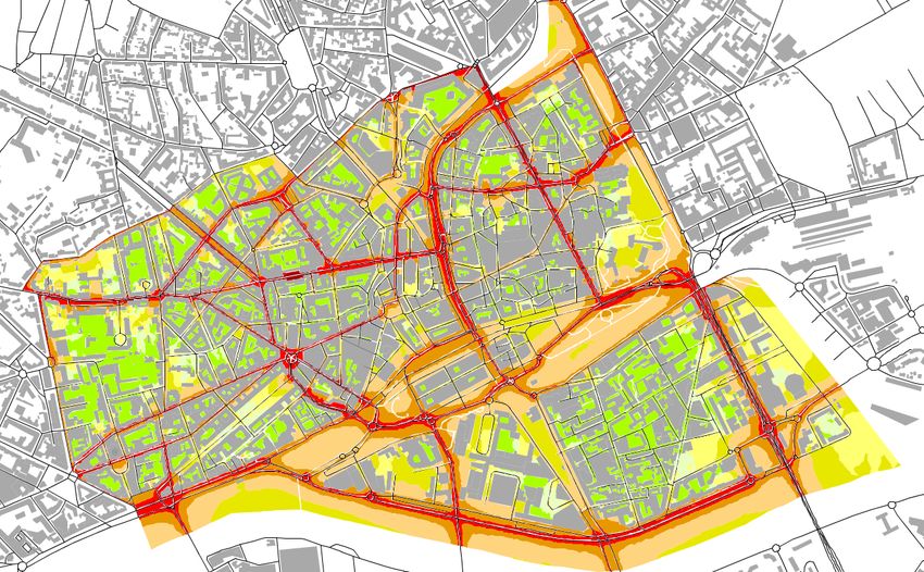
ISPRS Int. J. Geo-Inf. 2019, 8, 130                                                                 2 of 30

exposure [8], noise intermittency [9] or low frequency noise [10]. However, it should be noted that,
to a lesser extent, noise annoyance and some noise effects may come from other sound sources, such as
community noise [11], industrial noise [12] or recreational and leisure noise [13]. Lastly, the total
annoyance can also be the result of combined noise, such as between road traffic and industrial noise
sources [14].
      In response to these major health and societal challenges, the European Union implemented in
2002 the Directive 2002/49/EC [15], relating to the assessment and management of environmental
noise. The goal is to define an EU common approach to avoid, prevent or reduce the harmful effects
due to environmental noise exposure, mainly due to transportation and industrial sources. On the
basis of all the data acquired through the application of this directive, in 2012, almost 122 million
inhabitants were subject to noise levels above the limit of 55 dB(A), which is the threshold to consider
the first health effects of noise on inhabitants, including 14 million at extremely annoying levels [16].
This justifies why studies are still needed to reduce noise pollution, whether in relation to road, rail
and air traffics, or industrial activities (see, for example, [14,17–19] for recent studies).
      In the context of the Directive 2002/49/EC [15], noise maps are the main tool for investigation
and decision-making in the implementation of action plans to reduce noise pollution [20]. At present,
noise maps are obtained using numerical simulations, with software specifically developed for
environmental noise mapping, based on acoustic emission models of transportation and industrial
noise sources as well as propagation models. These emission and propagation models are derived from
national standards, such as DIN 18005-1 (Germany [21]), NMPB-08 (France [22,23]) or NORD 2000
(Denmark [24,25]). At the European level, harmonised standards were also proposed, such as
Harmonoise [26,27], or more recently the CNOSSOS-EU model (“Common Noise Assessment Methods
in Europe”) [28], which should become the reference model in Europe from 31 December 2018. Other
approaches, based on measurement (using fixed sensor networks [29] or participatory measurements
with smartphones [30–32]) or social data [33], are beginning to emerge, but will still require coupling
with numerical models [34] to be able to test action plans, as required by the European directive.
The usual numerical methods will remain the reference approach for a very long time, until the
approaches evolve and the standards change. Presently, improving calculation methods and noise
map representation are therefore still very important issues.
      Noise mapping based on numerical simulations requires beforehand a huge amount of
information concerning the investigated area, based on third-party data or models. Firstly,
the generation of the noise emission requires the knowledge of the road network including the
speed limits, the signage and the traffic flow on each road section. Secondly, the sound propagation
model requires data about the type of buildings, in addition to both the topography and soil landscape.
Thirdly, statistical data are needed in terms of population distribution and location of offices and
business activities. Because noise prediction models rely on geometric calculations, a fine description
and accurate quality of the geometric data (i.e., roads, buildings. . . ) are required, otherwise it would
be impossible to evaluate noise levels [35,36]. Therefore, the manipulation of all these data through
Geographic Information System (GIS) seems obvious to facilitate the production of noise maps [20]
(Chapter 10). In addition, the evolution of GIS technologies makes it possible to share the results with
citizens and decision-makers thanks to the standards and geographical services distributed over the
Internet, through Spatial Data Infrastructure (SDI) platforms [37,38]. As Abramic et al. [39] pointed
out, applying SDI techniques for noise mapping strategies permits also encoding data in a similar
manner, thus achieving semantic interoperability between models. In addition, SDI offers a natural
way to expose and share data on the web. This clearly shows the potential interest of integrating the
production of noise maps directly within a GIS, and not in parallel, as is currently the case by coupling
the inputs and outputs of noise mapping software with GIS platform. Such implementation could
considerably facilitate the evaluation and implementation of action plans to reduce noise [20] (Chapters
10–12). Lastly, as underlined by King and Rice [40], the philosophy behind the European directive
2002/49/EC, and more generally the context of the European directive INSPIRE [41], also motivates
ISPRS Int. J. Geo-Inf. 2019, 8, 130                                                              3 of 30

the use of open-source GIS [42], instead of black box implementations of comparable commercial
software packages.
      Thus, the present paper proposes an implementation of a simplified noise mapping approach
within a GIS, allowing to produce noise maps at a city or urban agglomeration scale with limited
calculation times, in order to consider several planning scenarios within reasonable duration.
The proposed method relies on a simplified implementation of the French national method ‘NMPB-08”,
but a similar approach could be considered for other national or international standards.
      After a review of existing noise mapping solutions and an analysis of the main scientific and
technical barriers in Section 2, Section 3 presents the French standard method and, in Section 4,
its implementation within the open source GIS platform OrbisGIS (website: http://www.orbisgis.org/)
in the form of a plugin, named NoiseModelling (website: http://noise-planet.org/noisemodelling.
html) (formerly NoiseM@p). A full application of NoiseModelling to the study of urban mobility plan
impacts in terms of noise exposure is finally shown in Section 5. This application was carried out
within the framework of the Eval-PDU project 2008–2012 (see, e.g., [43,44]). Three scenarios were
selected by the project consortium for their potential impacts in several societal, economical and
environmental concerns, and are thus investigated in the present paper in terms of noise impact by
means of dedicated methodologies managed entirely through an open source GIS tool.

2. Noise Mapping Issues

2.1. Existing Noise Mapping Solutions
      Nowadays, most strategic noise maps are produced by means of standard methods, as mentioned
in the Introduction. Such methods use constraints to break down the road infrastructure into segments
of approximately constant cross-section, thus describe each road section as a set of incoherent point
sources, and lastly compute noise attenuation along the propagation path between each point source
and an observation point. In contrast, no recommendation or peer-reviewed article specifies the
geometrical aspects concerning the research of the relevant propagation paths between sources and
receivers by ray tracing techniques. Some practical and specialist skills are yet developed by software
developing companies, as suggested by a few conference papers [45,46].
      Otherwise, the use of a Geographic Information System (GIS) software for the purpose of
noise mapping appears essential to harvest all required spatial data and to compute exposure
indicators [20] (Chapters 10–12). Prior to the establishment of the Directive 2002/49/EC [15],
De Kluijver and Stoter [47] underlined the need in a standardized method in Europe for the purpose
of noise forecasting and highlighted the virtues of a GIS integration for data collection, storage and
querying. To our knowledge, the first application of a GIS tool for the forecast of environmental noise
was established about two decades ago by Reijnen et al. [48] who studied the impact of road traffic
noise on breeding birds over a large area in the Netherlands. Thereafter, few authors experimented
on the integration of a road traffic noise model into a GIS. Thus, Li et al. [49] proposed a GIS based
traffic noise system implemented in the commercial GIS software ArcView (renamed latter ArcGIS)
including a few extensions and designed it for noise prediction in China. Unfortunately, the model
is implemented using a proprietary high-level algorithmic language (AVENUE), which does not
allow the portability of the application to other GIS systems. Pamanikabud and Tansatcha [50]
developed two traffic noise prediction models based on the UK’s standard CoRTN [51] and on the US’s
standard FHWA [52] that are also integrated in the previously mentioned commercial GIS system with
the same programming language, implying the same inconvenience as the preceding development.
Similarly, Gulliver et al. [53] developed an open-source tool for road traffic noise modelling that is
integrated in ArcGIS too. One can also cite the works by Reed et al. [54] who proposed an open-source
application, named SPreAD-GIS, dedicated to the modelling of anthropogenic noise propagation in
natural ecosystems. The application was implemented in Python as a toolbox in the ArcGIS software,
and is based on the System for the Prediction of Acoustic Detectability (SPreAD) developed by the US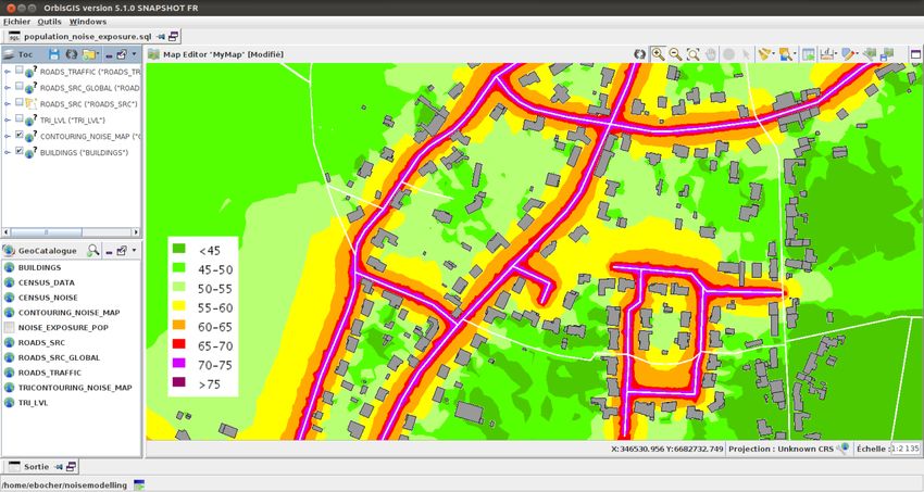
ISPRS Int. J. Geo-Inf. 2019, 8, 130                                                                4 of 30

Forest Service (USFS) and Environmental Protection Agency (EPA). Therefore, no full open-source
framework currently exists for the purpose of noise mapping at the territory scale.
     Moreover, further improvements are necessary to make large scale noise maps, at an
agglomeration scale for instance, within the END framework. One of the first optimizations concerns
the ray-tracing calculations between the receiver and the set of contributing sound sources [55],
which proves to be more efficient in the case of an equidistant segmentation of the line sources.
For large scale domains, it is necessary to limit the computation area. Since a fixed search radius
approach is likely to overlook significant noise sources, Probst (2008) [45] preferred the so-called
maximum error approach, for which the geometrical paths are first sorted with respect to their length,
and the combination of the sources is carried out in increasing order of length. The author also
mentioned a projection method where straight lines connect the receiver to the outermost edges of
all objects between the receiver and the source. It is reported that the method must be restricted to a
maximal distance from a source or from a receiver.
     Consequently, the prevision and mapping of environmental noise within the framework of the
END directive still require some improvements in terms of numerical optimization such as the search
for propagation paths between the sound sources and the receivers. The integration of both the
noise emission and propagation models into a GIS offers many advantages, particularly concerning
the management of the input and output data and the linkage with population data. However,
some scientific and technical barriers need to be overcome for this purpose.

2.2. Scientific and Technical Barriers
      The main scientific and technical barriers for the purpose of fulfilling at once the European noise
and the environmental data-related regulations, i.e., directives 2002/49/EC (END) and 2007/2/EC
(INSPIRE), respectively, concern the accessibility to the data, in particular in terms of standards
compliancy, interoperability and open data. In addition, some information is often lacking regarding
the physical properties of the various elements that make up the environment. For example, the nature
of the land plots are usually poorly defined or unknown. Indeed, if a vast amount of data were
now available, thanks to open data, its integration into modelling tools would remain a long and
complex task due to their quality, regarding positional uncertainty, temporal accuracy, covered area,
and attribute description [56,57]. Recent works and technologies should allow addressing this issue in
the near future (see, e.g., [58]). Likewise, the properties of the building facades, which are currently
deduced from another source of information (e.g., type or age of the building, and location of services),
could also be provided through open data portals or community databases such as OpenStreetMap.
Indeed, there is a general movement toward open data access [59]. For environmental assessment,
it induces new challenges, for example, the necessity to develop data processing techniques to capture,
document and collect data coming from various providers. GIS tools are once again well adapted to
solve this issue.
      Moreover, the calculation of sound levels requires significant computing resources. Nevertheless,
the computational burden can be addressed by optimizing the implementation of the computational
core, e.g., by multithreading the processes and threads as experimented by Probst [46] and by
Salomons et al. [60]. Besides, the noise annoyance is not only related to sound levels but also to
their time variations. Some improvements are thus still required to account for the noise dynamics by
integrating more advanced indicators and adapted mapping representations (see, e.g., [61]). Lastly,
the modelling of traffic-related noise at the urban scale relies on a few simplifications and hypotheses
of both the noise emission and propagation phenomena detailed hereinafter.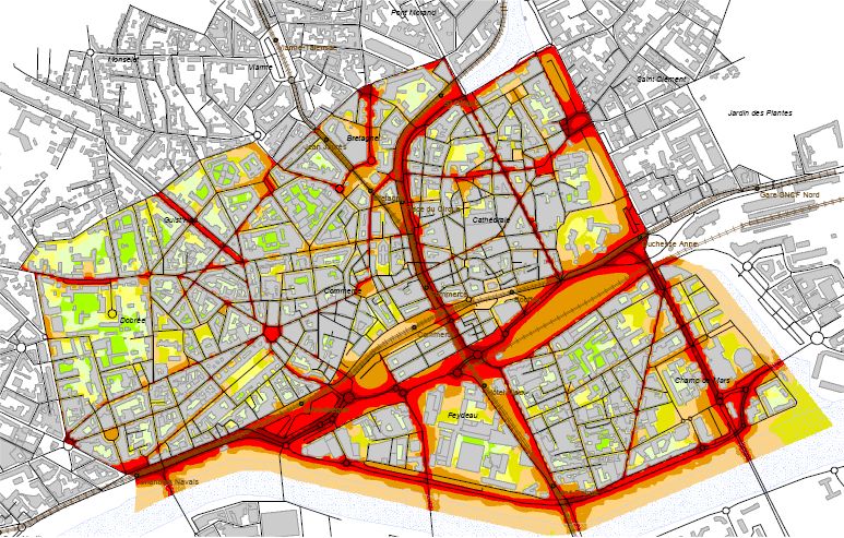
ISPRS Int. J. Geo-Inf. 2019, 8, 130                                                                 5 of 30

3. Noise Mapping Approach

3.1. Principle and Hypotheses
       As mentioned in the Introduction, the present approach is based on a simplified implementation
of the French national method “NMPB-08”, which consists in two steps: the estimation of traffic
noise emission over the transport network [62] (see Section 3.2) and the calculation of sound levels
over a receivers grid issued from the propagation from these noise sources to each receiver [63]
(see Section 3.3).
       Each implementation component is based on a few hypotheses in comparison to these two latter
methodological guides for reducing the computational burden and addressing the lack of input data.
Concerning the noise emission, the main simplifications relate to the description of the type and the
age of the road pavement, the stopping and starting road sections, the vehicles kinematic, and the
distribution between traffic of light and heavy vehicles over the various daily time periods, due to the
lack of related data. Nevertheless, the majority of the roads in built-up area consists of non-draining
(i.e., non-porous) surfaces, these latter being mostly used for road segments with vehicle speed over
70 or even 90 km/h. Other types of surfaces (e.g., rubberized asphalts) are therefore not considered.
This missing information in terms of input data also affects the sound propagation modelling since
land use data are often defined using another geographical reference frame as other dataset, making it
difficult to merge them with each other. Thus, the ground is considered as perfectly reflecting. Besides,
the approximations of the propagation calculations also concern the 2D modelling instead of 3D
computations, which implies locating the sound sources near the ground and the receivers on the same
horizontal plane as the sources. Thus, the reflected and diffracted fields remain on a same plane parallel
to the ground. Therefore, the horizontal diffraction by the vertical edges of the buildings is taken into
account (i.e., the sound rays propagate around the buildings), whereas the vertical diffraction by the
horizontal edges are neglected (i.e., the sound rays cannot propagate over the buildings). However,
the impact of this latter simplification on the prediction is relatively weak in densely multi-sourced
environment as encountered in urban area where the direct and reflected components of the sound field
largely predominate over the diffracted component. Since meteorological effects affect ground effects
and vertical diffraction, which are neglected for the above-mentioned reasons, only homogeneous
atmospheric conditions are considered.

3.2. Noise Emission
     The proposed implementation of the noise emission is based on the methodology detailed in the
guide published by the Sétra [62] for road vehicles. The noise generated by tramways is not addressed
in this methodological guide. However, this transportation mode is treated in the German directive
Schall 03 [64]. Thus, the method defined in the guide book of the Sétra [62] is extended in the present
work to tramways according to the German directive.

3.2.1. Point Sources Decomposition
     The noise emission depends on the Vehicles Categories (VC), which distinguishes Road Vehicles
(RV), gathering Light Vehicles (LV) and Heavy Trucks (HT), and Tramways (TW). The proposed
implementation consists in breaking down the line sources (i.e., the traffic and railway flows) into a
series of NS point sources Si (i = 1 to NS ) as depicted at Figure 1.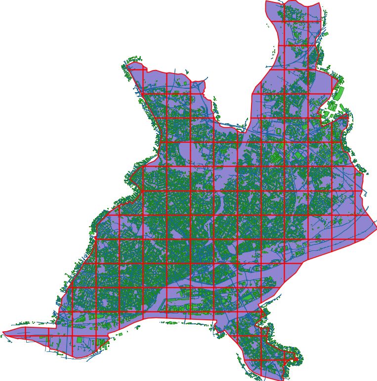
ISPRS Int. J. Geo-Inf. 2019, 8, 130                                                                  6 of 30

                           Figure 1. Breakdown of a line source into a series of point sources.

     The sound emission level of a point source Si is determined for a given frequency band j according
to the acoustic power level LW/m per metre of a line source, by the formula:

                                                  j       j
                                                LW,i = LW/m + 10 log10 di ,                             (1)

where di is the distance between two successive sources for the same line source. This distance is
selected in such a way as it complies with the rules defined by the reference method [62], namely:

                                                      di 6 0.5 × dmin,i                               (2a)
and
                                                      di 6 20 m,                                      (2b)

where dmin,i is the orthogonal distance between the point source Si and the nearest receiver point
Rnearest,i (see Figure 1).
      In our approach, the generation of the point sources is based on an equidistant breakdown of line
sources. The first point source Si=0 matches the entrance of the section, all next point sources being
                                          #    »
regularly spaced with a distance di = kSi Si+1 k. Depending on the distance to the end of the line source,
a last point source Si= NS may be added. When a new line source starts from the end of the previous
line source, the same process is applied. If the last point source of the previous line source coincides
with the first point source of the next line source, both noise level contribution are energetically added.

3.2.2. Sound Power Level Calculation
                                j
     The power level LW/m per metre for each point source is calculated as the energetic addition
(referred to by the symbol ⊕) of each VC contribution, that is:

                                       j          j                        j
                                                h                            i
                                      LW/m = ⊕ ∑ LW/m,VC + 10 log10 QVC + RVC .                         (3)
                                                 VC

      An energetic addition is defined as:

                                         L A ⊕ L B = 10 log10 10 L A /10 + 10 LB /10 .                  (4)

     The contribution of each VC corresponds thereby to the sum of the spectral distribution of the
                 j
emission power RVC , given per third octave bands in Table 1, and of the emission powers per metre of
lane LW/m,VC for an unit flow rate, weighted by the average hourly flow rate QVC .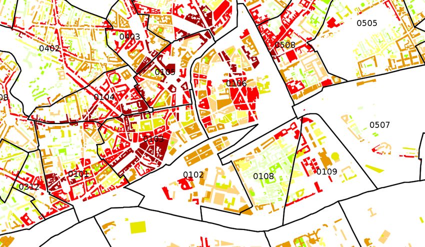
ISPRS Int. J. Geo-Inf. 2019, 8, 130                                                                                             7 of 30

                                                                         j
      Table 1. Spectral distribution of the emission power RVC (in dB(A)) of an elementary point source for
      RV (i.e., LV and HT) over non-porous surfaces and for TW at third octave bands of central frequencies
      f c (in Hz).

             f c [Hz]              100     125       160          200         250     315        400        500          630
             RRV [dB(A)]      −27         −26      −24           −21         −19     −16      −14          −11          −11
             RTW [dB(A)]      −11.3       −11.3    −11.3         −11.3       −11.3   −11.3    −11.3        −11.3        −11.3
             f c [Hz]              800      1k      1.25k        1.6k         2k      2.5k       3.15k      4k           5k
             RRV [dB(A)]       −8          −7       −8           −10         −13      −16     −18          −11          −23
             RTW [dB(A)]      −11.3       −11.3    −11.3         −16.3       −16.3    16.3    −21.3        −21.3        −21.3

                                                                                                             j
      Concerning RV, the emission power per metre of lane for an unit flow rate LW/m,RV is calculated
                                                                                                       j
at frequency j by breaking down the contributions of rolling noise Lr,W/m,RV and mechanical
         j
noise Lm,W/m,RV :
                                              j              j                   j
                                             LW/m,VC = Lr,W/m,VC ⊕ Lm,W/m,VC .                                                     (5)

      These two contributions depend on both the speed v (in km/h) and pace (i.e., steady speed and
acceleration) of the vehicle. Correction factors are introduced to take into account the age a (in years)
of the road pavement concerning the rolling noise, and the road declivity p (in %) for mechanical noise.
      For TW, the noise emission is mainly related to rolling noise, which is introduced similarly as the
road vehicles implementation, yet by neglecting the accelerating effect. Besides, a correction is applied
if an anti-vibration base is present (e.g., a floating slab).
      The calculation of the rolling noise for all VC (i.e., LV, HT and TW) and of the mechanical
contribution for RV (i.e., LV and HT) are detailed in Tables 2–5.

      Table 2. Rolling noise components of the emission powers per metre of lane for LV and HT at speed v
      (between 20 and 130 km/h) with their respective corrections associated with the age a (in years) of the
      road segment (the formulas correspond with the surfacing category R2 in the methodological guide of
      the Sétra [62] (Tables 2.4–2.6)).

                                                                              Correction [dB(A)]
                             RV          Lr,W/m,RV [dB(A)]
                                                                    a 6 2 Years       2 < a < 10 Years
                             LV       55.4 + 20.1 log10 (v/90)           −2.0          0.25 × ( a − 10)
                            HT        63.4 + 20.0 log10 (v/80)           −1.2         −0.15 × ( a − 10)

      Table 3. Mechanical noise components of the emission powers per metre of lane for LV and HT
      at steady speed according to v with their respective corrections according to the declivity p (in %,
      with Ascent (Asc.) and Descent (Desc) declivities) of the road segment (the methodological guide
      considers accelerating and decelerating road sections too [62] (Tables 2.8, 2.9 and 2.11)).

                                                                                     Correction [dB(A)]
             RV         v [km/h]         Lm,W/m,RV [dB(A)]                                Asc.                Desc.
                                                                    0 6 p 6 2%
                                                                                       2 < p < 6%          2 < p < 6%
                         20–30        36.7 − 10.0 log10 (v/90)               0               0                      0
             LV          30–110        42.4 + 2.0 log10 (v/90)               0               0                      0
                        110–130       40.7 + 21.3 log10 (v/90)               0               0                      0
                        20–70         49.6 − 10.0 log10 (v/80)
             HT                                                              0          2 × ( p − 2)             ( p − 2)
                        70–100         50.4 + 3.0 log10 (v/80)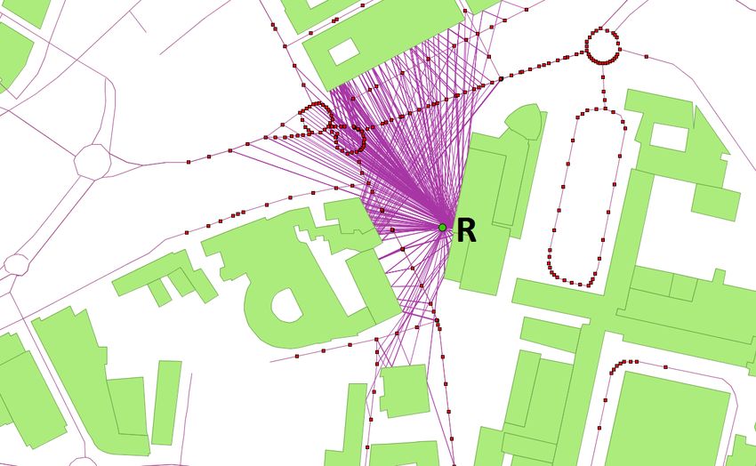
ISPRS Int. J. Geo-Inf. 2019, 8, 130                                                                                      8 of 30

      Table 4. Mechanical noise components of the emission powers per metre of lane for LV and HT at
      starting section according to the declivity p (in %, with Ascent (Asc.) and Descent (Desc) declivities) of
      the road segment.

                                      RV   Declivity p [%]                     Lm,W/m,RV [dB(A)]
                                      LV    all declivities                           51.1
                                              06p62                                   62.4
                                      HT   Asc. 2 < p < 6                 62.4 + max [2 × ( p − 4.5) , 0]
                                           Desc. 2 < p < 6                            62.4

      Table 5. Emission powers per metre of lane for tramways (TW) according to the ground type with the
      corrections associated with the nature of the rail base.

                                                                                            Correction [dB(A)]
                      Ground Type             LW/m,TW [dB(A)]
                                                                                       Classic Base      Absorber Base
                           Rigid           78.0 + 26.0 log10 (v/40)
                                                                                           0.0                 −2.0
                           Grassy          75.0 + 26.0 log10 (v/40)

3.3. Noise Propagation
     The modelling of the noise propagation relies on the methodological guide published by the
Sétra [63]. The sound propagation from a point source to a receiver is submitted to various phenomena
such as the geometrical spreading due to the expansion of the wavefront and the atmospheric
absorption that results from the molecular relaxation effect. The propagation can be modelled by
separating the contributions of each phenomenon, which leads to consider the sound field received at
a given location as a combination of:

•     the direct field, which corresponds to the sound waves propagating directly from the source to
      the receiver (Figure 2a);
•     the diffracted field, related to the diffraction of the sound waves around and over the buildings
      (Figure 2b); and
•     the reflected field, associated with the reflections on the ground and on the buildings facades
      along the propagation path that can also include absorption by these elements (Figure 2c,d).

    In the present implementation, the noise propagation is modelled as described in the
                                             j
methodological guide [63]. The sound level L R ,i at a receiver Rk from a point source Si , characterised
                                                                   k
                           j
by a power level LW,i as defined in Equation (1) for a given frequency band j, is evaluated from
the formula:
                         j       j                 j          j      j
                       L R ,i = LW,i − AdivR ,i − AatmR ,i − Adif − Agrd ,                     (6)
                                      k                        k                   k             Rk ,i      Rk ,i

where the attenuation terms refer to the respective contributions of the geometrical spreading (Adiv ),
the atmospheric absorption (Aatm ), the horizontal diffraction around the vertical edges of obstacles
(Adif ) and the ground effect (Agrd ).
      The geometrical spreading Adiv corresponds to the natural attenuation of noise during
propagation over a distance di , which is expressed as:

                                                AdivR          = 20 log10 (di ) + 11.                                       (7)
                                                        k ,i

    The atmospheric absorption Aatm is given as a function of the frequency-dependent atmospheric
absorption coefficient αair (ISO 9613-1:1993 [65]), namely:

                                                         j                          di
                                                    AatmR                 = αair        .                                   (8)
                                                                   k ,i            1000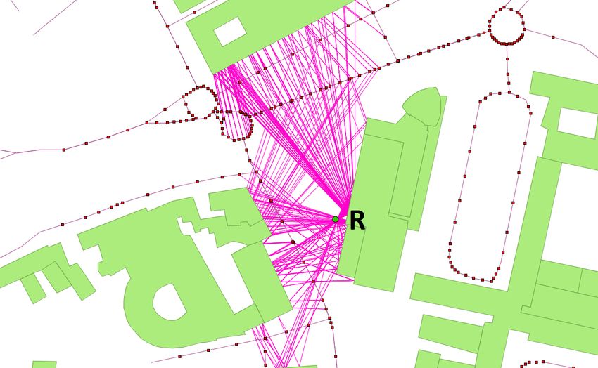
ISPRS Int. J. Geo-Inf. 2019, 8, 130 9 of 30
(a) Direct propagation (b) Horizontal diffraction (first-order)
(c) Specular reflection (first-order) (d) Specular reflection (second-order)
Figure 2. Illustrations of the propagation paths between the point sources (red) and a given receiver
point (green) for each contribution to the total sound field: (a) direct path; (b) first-order horizontally
diffracted path; and (c,d) first- and second-order specularly reflected paths.
The horizontal diffraction Adif around the vertical elements (e.g., the building edges) depends
on the path length difference δ (expressed in m) between the direct and diffracted propagation paths
(see Figure 2b) and is given by the relation:
10 log 40 00 40 00
j 10 3 + λC δ if λC δ > −2,
Adif = (9)
R k ,i 0 otherwise,
where λ stands for the wavelength of the center frequency for the considered frequency band and C 00
is a coefficient used to consider multiple diffractions (nth
dif - order) such as:
1 if ndif = 1 (single diffraction),
C 00 = 2 (10)
1+(5λ/e) 2 if ndif > 1 (multiple diffraction) and e > 0.3 m,
1/3+(5λ/e)
with e the distance between the first and last diffractive edges. The path length difference δ is calculated
by means of a “corner-to-corner” propagation technique with an offset of a few centimetres in relation
to the wall (the offset is required since the sound ray would be rejected by the algorithm if it collides
with a wall).
Both the reflected and diffracted fields on vertical surfaces are modelled by introducing an
order of reflection nref and an order of diffraction ndif , respectively, which correspond to the
number of reflections and diffractions that are taken into account from the source to the receiver
(see Figure 2). In addition, one can also limit the number of reflections and diffractions, in the
calculation, by considering an extra parameter dlim for the maximal distance between the source and
the corresponding vertical surface (see Section 4).
The ground effect Agrd is also simplified in comparison to the standard methodology detailed
in the guide Sétra [63] since the soil nature is often unknown. Thus, the grounds are considered as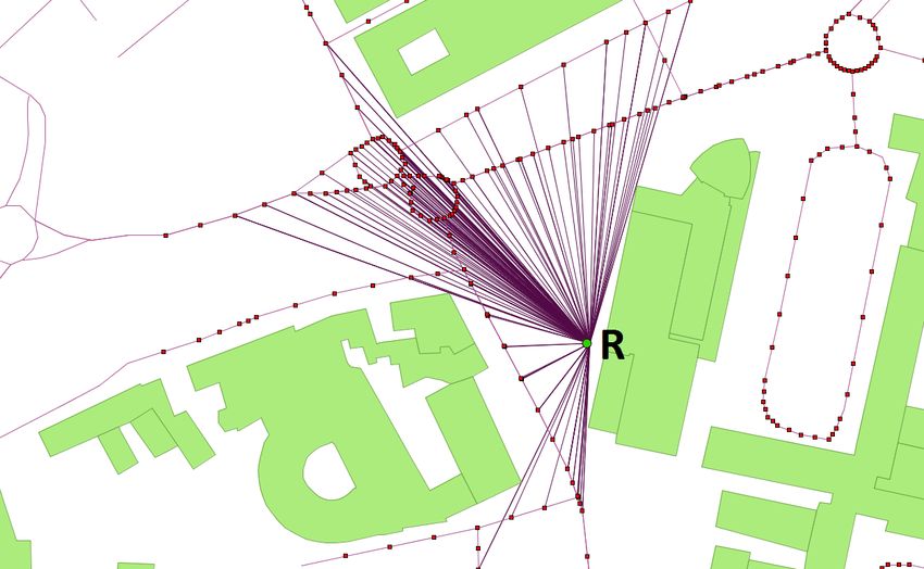
ISPRS Int. J. Geo-Inf. 2019, 8, 130                                                                                   10 of 30

perfectly flat (i.e., without a specific topography) and reflecting, with AgrdR                      = −3 dB, which tends to
                                                                                              k ,i
slightly overestimate the overall noise levels.
     Besides, the potential specular reflections (nth
                                                   ref - order) from the vertical surfaces (e.g., facades,
                                                                                                            j
noise barriers, etc., see Figure 2c,d) are considered by correcting the power level LW,i of the sound
source in Equation (6) according to the absorption coefficient αvert of the considered surfaces, namely:

                                       (n )      ( n −1)
                                      LW ref = LW ref      + nref × 10 log10 (1 − αvert ) .                              (11)
                                         Si        Si

      Each specular reflection is modelled by means of the image receiver method.

3.4. Numerical Optimisation
    In addition to the simplifications made to the modelling of both the noise emission (Section 3.2)
and propagation (Section 3.3), a few numerical optimisations were designed to reduce the
computational burden related to the calculation over large computational domains.

3.4.1. Domain Subdivision
     Owing to the extent of the investigated areas (e.g., a huge agglomeration), a breakdown of the
computational domain into subdomains is achieved to reduce the memory requirements, as illustrated
in Figure 3. The computational domain is divided into 2n subdomains in relation to the global envelope
as long as the maximal propagation distance (see Section 3.4.2) remains lower than a ratio equal to
30% of the maximal dimension of a subdomain. Thus, a weak ratio produces few subdomains and
requires consequently a huge amount of memory but is more efficient in terms of calculation time.
On the contrary, a higher ratio generates a lot of subdomains and therefore necessitates less memory
but induces lower computation times. A ratio of 30% is a good compromise that allows to reduce the
memory requirements while keeping reasonable calculation time.

             (a) Domain subdivision                                         (b) Calculation points

      Figure 3. Illustrations of: (a) the decomposition of the domain into sub-domains; and (b) the definition
      of the calculation points on the basis of an adaptive meshing of a sub-domain.

     Each subdomain is then meshed with a thin and adaptive triangulation method in order to
build the grid of calculation points (i.e., the point receivers). This triangulation process handles the
continuity between the subdomains, in order to recompose, at the end of the process, the noise map on
the whole domain. In addition, one can also adjust the maximum size of a mesh, and a grid refinement
at the vicinity of the traffic lanes, using specific meshing parameters smax and droad , respectively
(see Section 4.2.2).
     The subdivision depends on two parameters: the size of the calculation domain (i.e., the area
covered by the receivers) and the limit value of source–receiver propagation (parameter dmax in
ISPRS Int. J. Geo-Inf. 2019, 8, 130 11 of 30
Section 4.2.2). The continuity between subdomains is ensured by taking into account the “active”
sound sources from adjacent subdomains (Figure 4). This subdivision process is only required for
large computational domains. Besides, in certain cases, the need in acoustic indicators calculations is
limited to a few fixed observation points, which reduces the computation time (no mesh or building
up of subdomains, and limitation of the number of receivers).
Figure 4. Search of the “active” sound sources (red) for a given receiver point R (green). An “active”
sound source may be located in adjacent subdomains.
3.4.2. Point Source Generation
One of the major original features of the present approach rests upon the construction of the
point sources for each calculation point and not for all the receivers points, as depicted in Figure 5.
This allows reducing the amount of point sources required at each calculation point, in respect of
Equation (2). Besides, for the same purpose of limiting the amount of calculations, only sound sources
located within a critical radius centred on each calculation point are considered.
Figure 5. Example of the consideration of the point sources (in blue) for a given receiver R (in green).
The discretisation of the line sources depends on the distance from the receiver.ISPRS Int. J. Geo-Inf. 2019, 8, 130 12 of 30
Furthermore, according to the distance between a receiver and a noise source, this latter can lead
to a very weak contribution to the sound level at the receiver. It is generally acknowledged that the
maximal source–receiver distance must be comprised between 500 m and 1 km. However, the radius
around which the sources are taken into account influences the calculation time. In most cases for
which a sound source is located at the vicinity of the receiver, the more remote sources will have a
minimal impact. A criterion was then designed, which consists in estimating the gain in terms of
sound level of a hypothetical source i with a power WS located at a distance dmin from the receiver.
This criterion is defined by considering a free-field propagation and by neglecting the atmospheric
attenuation, that is: !
WS L R /10
10 log10 2
+ 10 − L R < e, (12)
4πdmin
where L R is the current sound level at receiver R due to all the active sources i with dmin,i < dmax /6,
where dmax is the maximal source–receiver distance that is allowed for the computation (i.e.,
a calculation parameter; see Section 4.2.2). Thus, when this criterion is fulfilled, all the real sources in
this new additional active zone are considered and, thus, used to update the sound level L R at receiver
R. An another hypothetical sound source is introduced at a larger distance dmin from the receiver and
the criterion is checked again. The process is repeated again until the value of the distance from the
receiver dmin reached the maximal source–receiver distance dmax .
In practice, the value of the power level WS and of the parameter e are fixed at 94 dB(A)
and 0.03 dB(A), respectively. The values of the distance dmin is chosen on a given range
[dmax /5, dmax /4, dmax /2, dmax ]. These parameters seem to give relevant results, but can be modified
depending on the urban configuration.
4. Integration within the OrbisGIS Platform
4.1. Architecture
The proposed prediction method is implemented in an open source GIS ecosystem. As described
in Figure 6, the general framework consists of three main modules, written in JAVA: the NoiseModelling
plugin, the H2 database (website: http://h2database.com/) with its H2GIS extension (website: http:
//www.h2gis.org/) [66] and the OrbisGIS platform [67].
Figure 6. NoiseModelling framework.
NoiseModelling is organized in two modules. The NoiseModelling core contains the main
algorithms for both the sound levels and noise maps calculations. The first part evaluates the noise
emission related to the road and rail traffic, as detailed in Section 3.2. The second part computesISPRS Int. J. Geo-Inf. 2019, 8, 130 13 of 30
the noise propagation from each point source to potential receivers, according to the simplified
standard-based model described in Section 3.3, by taking as inputs:
• a set of sound sources defined by a geometry (lines or points) and an associated emission power
in the form of a third octave band spectrum within the frequency range from 100 Hz until 5 kHz;
• an array of buildings as a 2D geometry (polygons), without information requirement concerning
neither the buildings height nor the topography; and
• a list of parameters such as the order of reflection nref and the walls absorption αvert (Equation (11)),
the order of diffraction ndif (Equations (9) and (10)), or the maximum distance of propagation dmax .
The NoiseModelling SQL functions module exposes the core processes as a set of SQL functions.
These functions are implemented on top of the Relational Database Management System (RDMS) H2
and its spatial extension called H2GIS [66], and take thus benefits from optimised spatial functions
and indexes. The SQL functions are loaded by the H2GIS database that is used by the OrbisGIS
platform to store the data and to perform spatial analysis. The data model that stores and queries the
geographic features (geometry and attributes) uses the OGC (Open Geospatial Consortium) simple
feature specification [68,69]. The communication between the database and the GIS tools is carried
out from Java Database Connectivity (JDBC) API. The JDBC API provides standardized methods
to query and to update data in a database. Consequently, the H2GIS noise SQL functions could be
executed in another context, e.g., with a command line script in Python using Psycopg or in an Extract
Transform Tool like Pentaho Kettle that supports JDBC connection (the method for connecting H2GIS
to Pentaho Kettle is presented here: https://github.com/orbisgis/h2gis/wiki/4.1-Data-Integration-
Pentaho-Kettle).
Inside the OrbisGIS ecosystem, the noise functions are manipulated both from a web service
or a Graphical User Interface (GUI). When NoiseModelling is used as a web service, it is integrated
as standalone module that communicates with the database and the client (that sends the requests)
through OGC standards and JDBC protocol (Figure 7). To interact with the web service, the user must
use a client application that supports the WPS specification as QGIS (website: https://www.qgis.org)
offers. On the GUI side, NoiseModelling is managed from a SQL console that enables to execute SQL
requests and to build complex scripts. This console also proposes numerous additional features for
helping the user with code formatting or writing for example.
The GUI of OrbisGIS is based on the same architecture as the web service except that it runs on
a local server, invisible to the end-user. The processing chain takes profit of the GIS capabilities in
terms of database access (the database access allows interacting with both the input and output data),
geometrical calculations (H2GIS, OrbisWPS) and map rendering, cartography (OrbisMAP). As the
main component of the OrbisGIS ecosystem, H2GIS and its spatial functions allow to handle numerous
tasks such as:
• producing a continuous noise map as iso-levels based on the colour code defined in the standard
NF S31-130 [70]; and
• computing the population noise exposure by means of a spatial statistical analysis with external
data (for example, IRIS data from the French National Institute of Statistics and Economic Studies
(INSEE, https://www.insee.fr/en/accueil) or, at the European scale, GEOSTAT data from the
European Statistical Office (Eurostat—https://ec.europa.eu/eurostat/fr/web/gisco/geodata/
reference-data/population-distribution-demography/geostat)).ISPRS Int. J. Geo-Inf. 2019, 8, 130 14 of 30
Figure 7. NoiseModelling web service architecture.
4.2. Use of NoiseModelling from the GUI
NoiseModelling is available in OrbisGIS as a set of SQL functions. These functions are
encapsulated into SQL scripts and executed from the SQL console GUI illustrated in Figure 8.
Figure 8. OrbisGIS Graphical User Interface (GUI) and its Structured Query Language (SQL) console.ISPRS Int. J. Geo-Inf. 2019, 8, 130 15 of 30
Figure 9 describes the general data flow processing. Firstly, the data must be loaded from OrbisGIS
and, secondly, they are processed by the NoiseModelling functions. Then, the results stored in a H2GIS
database are queried by the OrbisGIS tools to create thematic maps (style rendering). At the end,
the data and their styling could be shared using geospatial standards (GeoJSON to export raw data,
and Symbology Encoding format to share map styles).
Figure 9. NoiseModelling data flow.
For demonstration purpose, a single approach to both perform a noise map and compute noise
exposure is presented hereinafter following three steps:
• Step 1: Compute sound sources from traffic data.
• Step 2: Create the noise map.
• Step 3: Estimate population exposure.
Each step is based on the use of SQL queries and functions that are fully documented in the
NoiseModelling documentation (website: https://github.com/Ifsttar/NoiseModelling/wiki).
4.2.1. Step 1: Compute Sound Sources from Traffic Data
To compute the sound sources, a table that represents the road network must be available in the
OrbisGIS platform. Table 6 shows the required input values for each geometry of the road network
data and for the same reference periods (see Section 5.2.1). Note that the geometries must be duplicated
to give sound level for each driving direction.
Table 6. Description of the road traffic input values.
Column Name Data Type Description
the_geom Geometry Polyline representing a road for a driving direction
lv_speed Double Average light vehicle speed
hv_speed Double Average heavy vehicle speed
lv_per_hour Integer Average number of light vehicles by hour
hv_per_hour Integer Average number of heavy vehicles by hour
begin_z Double Road start altitude
end_z Double Road end altitude
road_length2d Double Road length in 2 dimensions
Then, the beginning and end-z values are extracted from the road geometry and its 2D length is
calculated thanks to the H2GIS spatial function BR_EvalSource, by executing the SQL query given by
the Script 1 in Appendix A that creates the table roads_src_global.
A new table is next produced that contains, for each geometry, a noise emission value
expressed in dB(A) for light and heavy vehicles. The spectrum distribution is computed using
the BR_SpectrumRepartition function that expects three parameters:ISPRS Int. J. Geo-Inf. 2019, 8, 130 16 of 30
• a third octave band frequency among the values from 100 to 5000 Hz;
• an integer value, to set the category of the road surface (“0” for porous pavements and “1” for
non-porous pavement); and
• a noise emission value in dB(A).
Applied on the table roads_src_global previously created, the BR_SpectrumRepartition
function returns the third octave band levels in dB(A) for both vehicle emission spectra, as illustrated
by Script 2 in Appendix A. The result is stored in a new table called roads_src and used to build a
noise map.
4.2.2. Step 2: Create the Noise Map
The first step of the noise map creation consists in computing the noise propagation on the set of
Delaunay triangulation vertices that integrate road and building geometries. This stage is achieved by
using the BR_PtGrid function which receives 12 input parameters:
• the name of the building table, which contains a geometry column which type is POLYGON;
• the name of the table that stores the sound power level expressed in dB(A) for a geometry type
POINT or LINESTRING;
• the name of the emission level column;
• the maximum propagation distance (dmax , in meter) from the receivers that enables to ignore the
sources farther than this distance for each receiver (see Section 3.4.2);
• the maximum wall seeking distance (dlim , in meter), which permits to overlook walls farther than
this direct propagation distance between each source and receiver, thus neglecting reflections and
diffractions on these walls;
• the road width (in meter), which gives the distance from which the receivers start being created
(should be superior than 1 m);
• the receivers densification value (droad , in meter), which creates additional receivers at the
corresponding value from the sources (0 to disable);
• the maximum area of a triangle (smax , in squared meters), which sets the maximum surface for
the noise map triangular mesh (a smaller area means more receivers;
• the sound reflection order (nref , a positive integer), which corresponds to the maximum number
of wall reflections between each source and receiver;
• the sound diffraction order (ndif , a positive integer), which defines the maximum number of
horizontal diffractions between each source and receiver; and
• a wall absorption value (αvert , a real value between 0 and 1).
As depicted in Figure 10, the BR_TriGrid function produces a constrained Delaunay triangulation
by executing Script 3 given in Appendix A.
In addition to its geometry, each triangle is defined by five values stored in a table with the
following columns:
• TRI_ID, unique identifier of a mesh (i.e., a triangle);
• W_V1, sound energy for the receiver at the first vertex of the mesh;
• W_V2, sound energy for the receiver at the second vertex of the mesh;
• W_V3, sound energy for the receiver at the third vertex of the mesh; and
• CELL_ID, unique identifier for a cell if the computational domain is subdivided (default is 0;
see Section 3.4).
The output triangles are then merged to compute a noise contour map. The process, presented in
SQL Script 4 in Appendix A, takes advantage of the SQL language and of the spatial functions
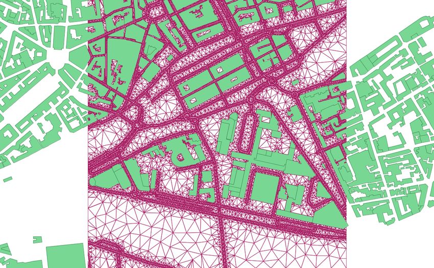
ST_TriangleContouring, ST_Union, ST_Accum and ST_Explode. Figure 11 shows the producedISPRS Int. J. Geo-Inf. 2019, 8, 130 17 of 30
contour noise map for a maximum propagation distance equal to 750 m, a maximum wall seeking
distance of 50 m, roads width of 1.5 m, a receivers densification value equal to 2.8 m, a maximum area
of triangles of 75 m2 , a sound reflection order of 2, a sound diffraction order equal to 1 and a wall
absorption value equal to 0.23 (concrete vertical surfaces).
Figure 10. Example of the results of the BR_TriGrid function in the OrbisGIS platform.
Figure 11. Contour noise map.
4.2.3. Step 3: Estimate Population Exposure
The population exposure is the most common indicator used to put in perspective a noise map
and the distribution of the population. These exposure rates correspond to the number of inhabitants
living in dwellings exposed to equivalent noise levels (i.e., Lden ) within standard value ranges. It could
be calculated from all noise level categories or from a level exceeding a value, according to the most
exposed facade (in this case, receiver points are placed at a distance of 1 m in front of the facade),ISPRS Int. J. Geo-Inf. 2019, 8, 130 18 of 30
as recommended in the french methodological guide of CERTU [71]. The spatial analysis functions
available in OrbisGIS allow computing the number of inhabitants for each noise level categories.
For example, SQL Script 5 in Appendix A details the method, using two input tables: the contouring
noise map and the location of inhabitants provided by the national institute of statistics and economic
studies (INSEE). These data are represented as a population grid dataset, where a cell contains a value
of inhabitants.
The distribution of the total of inhabitants per noise level could then be presented in a bar chart
or a table and integrated in an external document. All steps can be automated from the OrbisGIS
platform and then exposed as a set of services available from Open Geospatial Consortium standards
(WMS layer for data rendering, WPS service for data processing).
5. Application to the Study of Urban Mobility Plans
5.1. Urban Mobility Plans Scenarios
The proposed integration of the noise emission and propagation implementations into a GIS can
help decision-makers to estimate the impact of urban mobility plans in terms of noise annoyance and
population exposure. The present work falls within the framework of the Eval-PDU project which was
originated in response to a proposal of Nantes Métropole (an urban Metropolitan Community in France)
to conduct research concerning the assessment of the environmental impacts of urban mobility plans
for the City agglomeration [43].
The Nantes conurbation is served notably by three tramlines, one dedicated bus line and lots of
other bus lines, and promotes soft modes of transport with the development of pedestrian streets and
walkways, as well as bicycle lanes.
The Eval-PDU project considered not only the noise impact, but also other environmental effects
(air pollution and energy) and socio-economic (property values of housings, changes in citizen’s
behaviour, etc.). Several scenarios were processed and compared with the situation for the 2008
reference year (T0) in order to estimate changes in citizen’s displacement behaviour, due to variation
of energy price, urban sprawling, local and national economic transformations. Regarding noise,
only three scenarios leading a priori to a meaningful effect in terms of sound levels (i.e., T1, T2 and T4)
are considered, and are detailed in Table 7.
Table 7. Description of the reference situation T0 and of the three studied scenarios (T1, T2 and T4).
Code Description
T0 Situation for the 2008 reference year
Drop of the automobiles demand by removing 25% of the automobiles trips, which witnesses a
T1
loading rates for vehicles up 33%
T2 Increase in the travel demand up 20% (due to a 20%-growth of population or of the mobility)
T4 Doubling of the fuel price
5.2. Input Data
5.2.1. Traffic Data
The sound emission map is made of a point sources network based on traffic information
generated by a road traffic model and furnished by one of the partners of the Eval-PDU project.
The traffic model relies on road counts data as well as other input data that determine the distribution
of vehicle flows: the transport supply, the territorial socio-economic conditions, and household travel
surveys [44,72]. This model is able to describe the kinematics of both light vehicles and heavy trucks
over a major road network (5000 km) with a fine description of the traffic data, and over a secondary
road network (15,000 km) with a lower level of representation of the traffic. The territory is modelled
into IRIS zones in the study area and into municipalities in the rest of the department, which correspondISPRS Int. J. Geo-Inf. 2019, 8, 130 19 of 30
with the origin and destination points of the journeys. IRIS is a French abbreviations of aggregated
units for statistical information, and represents a geographic part of a commune.
However, the reference periods of traffic data (the traffic data include, for each reference period,
the required values listed in Table 6), obtained by the traffic model, which are defined by Night
Off-peak Hours (NOH), Day Off-peak Hours (DOH), Morning Rush Hours (MRH) and Evening Rush
Hours (ERH), differ from the reference periods for the calculation of the acoustic indicators. Indeed,
the acoustic reference periods and the related indicators are defined, in France, by the methodology
described in [71]: namely, the time slot 06:00–18:00 for the day with the corresponding A-weighted
long-term average noise level over one year Ld ; 18:00–22:00 for the evening with the related noise level
Le ; and 22:00–06:00 for the night with the corresponding noise level Ln . The correspondence between
both reference periods are summarised in Table 8. The three acoustic indicators are then used to
calculate the day–evening–night noise indicator Lden as recommended by the Directive 200/49/EC [15]
to assess noise annoyance, which is calculated for each frequency band j by summing the contributions
over the three acoustic time periods (the evening and night time slots are penalised, +5 dB and +10 dB,
respectively, to reflect the increased annoying effect of noise during these periods), that is:
j j j
" !#
j 1 L
d Le +5 Ln +10
Lden = 10 log10 12 × 10 10 + 4 × 10 10 + 8 × 10 10 . (13)
24
Table 8. Breakdown of “acoustic” reference periods from “traffic” reference periods.
Period 0:00 1 .a.m 2:00 3:00 4:00 5:00 6:00 7:00
Acoustic night day
RV NOH DOH MRH
TW NOH NOH DOH MRH
Period 8:00 9:00 10:00 11:00 12:00 1:00 2:00 3:00
Acoustic day
RV MRH DOH
TW MRH DOH
Period 4:00 5:00 6:00 7:00 8:00 9:00 10:00 11:00
Acoustic day evening night
RV DOH ERH DOH NOH
TW DOH ERH DOH NOH
The sound levels are thus calculated for each traffic reference period, that is LNOH , LMRH ,
j
LDOH and LERH , and then reconstructed for the acoustic reference periods for the Lden calculations.
The calculation of the day equivalent level, which is common for all VC (i.e., RV and TW), is thus
given by:
j j j
" !#
j 1 L
MRH
L
DOH L
ERH
Ld = 10 log10 2 × 10 10 + 9 × 10 10 + 1 × 10 10 . (14)
12
In contrast, the calculations of the evening and night equivalent levels depend on the VC (i.e.,
RV or TW) since the public transports does not work between 01:00 and 04:00 This leads to consider
two time intervals for TW, namely the time slots [08:00–01:00] as NOH1 and [04:00–06:00] as NOH2 .
The two acoustic indicators are thus computed for RV by:
j j j
" !#
L L L
j
L = 10 log 1 NOH DOH ERH
2 × 10 10 + 1 × 10 10 + 1 × 10 10 ,
e 10 4
(15)
j
j
Ln = LNOH ,ISPRS Int. J. Geo-Inf. 2019, 8, 130 20 of 30
and for TW by:
j
L j j
NOH1 L L
DOH ERH
1
Le ( j) = 10 log10 4 2 × 10 10 + 1 × 10 10 + 1 × 10 10
,
j j
(16)
L L
NOH1 NOH2
1
Ln ( j) = 10 log10 10 5 × 10 10 + 2 × 10 10 .
5.2.2. Other Input Data
Geographical data The geographical data (topography, buildings, roads) are issued from the BD
TOPO R database provided by the National Institute of Geographic and Forestry Information
(IGN, website: http://www.ign.fr/). Note that there is no noise barrier in the study area.
Road pavement Due to the lack of information concerning the nature of road pavements,
some simplifications in comparison to the standard method [62] are considered in terms of type
and age of the road pavement. Because porous surfaces are mostly used for road segments
with vehicle speed over 70 or even 90 km/h, only non-porous pavements are considered,
which represent the majority of the roads in built-up area. In addition, the age of pavement is
fixed at 10 years, which is, here again, a relevant hypothesis.
Population Statistical population units are given from INSEE databases with Commune boundaries
(INSEE, website: https://www.insee.fr/).
5.3. Initial Verification
A quantitative validation was difficult to implement as it would require to compare the produced
noise maps with “reference” noise maps issued from classical tools on the basis of similar input
datasets [73]. The relevance of such a comparison is anyway arguable since the “reference” noise
maps are often themselves not validated, neither in comparison with measurements nor with other
simulation tools, particularly for built-up areas. Consequently, the main interest of the noise maps
produced with the proposed simplified method rests rather upon the relative comparison of some
scenarios concerning urban transport plans in order to identify large differences in terms of noise
levels (i.e., in the order of several decibels).
Nevertheless, a “qualitative” verification was achieved here, which consists in comparing the
noise maps generated by the present approach with the ones produced by the agglomeration of Nantes
Métropole within the framework of the application of the Directive 2002/49/EC [15] for 2008, using a
commercial software. Thus, Figure 12 shows the day–evening–night equivalent sound levels Lden of
Nantes city centre obtained with both methods. Using NoiseModelling, the input parameters for the
sound propagation calculations (i.e., of the BR_TriGrid function) were the following: a maximum
propagation distance dmax = 750 m, a distance in searching for facades dlim = 50 m, a roads width
of 1.5 m, a receivers densification value droad = 2.8 m, a maximum area of triangles smax = 75 m2 ,
sound reflection and diffraction orders nref = 2 and ndif = 1 respectively, and a wall absorption
value αvert = 0.23 (concrete vertical surfaces). These parameters values were chosen as they ensure a
satisfactory compromise between calculation time and results convergence in the present application.
A good agreement appeared over most of the busy roads (higher levels in red) and in quiet
areas (lower levels in green). However, some non-negligible discrepancies could be noticed, of which
origin should result from very different input data concerning both the traffic and road networks,
revealing a high sensitivity to input datasets. In particular, the data issued from the traffic model
seemed to be too averaged for the secondary road network (identical average value for several roads
of the same district), while “real” traffic flows were different. These differences between the two maps
must nonetheless be tempered since the “reference” noise map rests upon its own hypotheses and
approximations in terms of both modelling and input data.You can also read