CASTLE: cell adhesion with supervised training and learning environment
←
→
Page content transcription
If your browser does not render page correctly, please read the page content below
Journal of Physics D: Applied Physics

PAPER • OPEN ACCESS

CASTLE: cell adhesion with supervised training and learning
environment
To cite this article: S G Gilbert et al 2020 J. Phys. D: Appl. Phys. 53 424002

View the article online for updates and enhancements.

                                 This content was downloaded from IP address 176.9.8.24 on 21/09/2020 at 21:25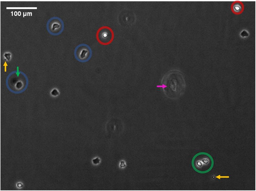
Journal of Physics D: Applied Physics
J. Phys. D: Appl. Phys. 53 (2020) 424002 (16pp) https://doi.org/10.1088/1361-6463/ab9e35
CASTLE: cell adhesion with supervised
training and learning environment
S G Gilbert1,2, F Krautter3, D Cooper4, M Chimen5, A J Iqbal3 and F Spill1
1
School of Mathematics, University of Birmingham, Edgbaston, Birmingham, B15 2TT, United Kingdom
2
EPRSC Centre for Doctoral Training in Topological Design, School of Physics, University of
Birmingham, Edgbaston, Birmingham, B15 2TT, United Kingdom
3
Institute for Cardiovascular Sciences, College of Medical and Dental Sciences, University of
Birmingham, Edgbaston, Birmingham, B15 2TT, United Kingdom
4
Centre for Biochemical Pharmacology, William Harvey Research Institute, Bart’s and the London
School of Medicine, Charterhouse Square, London, EC1M 6BQ, United Kingdom
5
Institute of Inflammation and Ageing, College of Medical and Dental Sciences, University of
Birmingham, Wolfson Drive, Birmingham, B15 2TT, United Kingdom
E-mail: SGG897@student.bham.ac.uk and f.spill@bham.ac.uk
Received 27 January 2020, revised 2 June 2020
Accepted for publication 18 June 2020
Published 29 July 2020
Abstract
Different types of microscopy are used to uncover signatures of cell adhesion and mechanics.
Automating the identification and analysis often involve sacrificial routines of cell manipulation
such as in vitro staining. Phase-contrast microscopy (PCM) is rarely used in automation due to
the difficulties with poor quality images. However, it is the least intrusive method to provide
insights into the dynamics of cells, where other types of microscopy are too destructive to
monitor. In this study, we propose an efficient workflow to automate cell counting and
morphology in PCM images. We introduce Cell Adhesion with Supervised Training and
Learning Environment (CASTLE), available as a series of additional plugins to ImageJ.
CASTLE combines effective techniques for phase-contrast image processing with statistical
analysis and machine learning algorithms to interpret the results. The proposed workflow was
validated by comparing the results to a manual count and manual segmentation of cells in
images investigating different adherent cell types, including monocytes, neutrophils and
platelets. In addition, the effect of different molecules on cell adhesion was characterised using
CASTLE. For example, we demonstate that Galectin-9 leads to differences in adhesion of
leukocytes. CASTLE also provides information using machine learning techniques, namely
principal component analysis and k-means clustering, to distinguish morphology currently
inaccessible with manual methods. All scripts and documentation are open-source and available
at the corresponding GitLab project.
Supplementary material for this article is available online
Keywords: machine learning, cell adhesion, cell morphology, galectins, imagej, ilastik, image
analysis
(Some figures may appear in colour only in the online journal)
1. Introduction
The function of almost all cell types, including leukocytes,
Original Content from this work may be used under the platelets, and cancer cells, critically involves a number of
terms of the Creative Commons Attribution 4.0 licence. Any
further distribution of this work must maintain attribution to the author(s) and mechanical processes [1]; these include the regulation of cell-
the title of the work, journal citation and DOI. cell and cell-matrix adhesion, flow sensing and changes in
1361-6463/20/424002+16$33.00 1 © 2020 The Author(s). Published by IOP Publishing Ltd Printed in the UK
J. Phys. D: Appl. Phys. 53 (2020) 424002                                                                                       S Gilbert et al

morphology during cell migration [2]. A particularly import-               automate the process with little human intervention to increase
ant case, where adhesions need to dynamically change on short              both speed and objectivity [9, 10].
time scales, involve the adherence of blood cells. For example,                In the present study, we test our workflow on different
leukocytes adhere to the endothelium and transmigrate out                  types of recently acquired data sets: we quantify adhesion and
into inflamed tissues, and platelets activate and adhere to a              morphology of peripheral blood mononuclear cells (PBMCs)
substrate or to each other during wound closure. To invest-                and polymorphonuclear leukocytes (PMNs) in dependence on
igate the effect of specific adhesion molecules on leukocyte               galectins, and platelet adhesion depending on von Willebrand
behaviour, e.g. those appearing on the endothelium, biolo-                 factor (vWF) with stimulation by a platelet agonist, adenosine
gists often employ flow based adhesion assays where cells                  diphosphate (ADP). Galectins are a family of ß-galactoside
adhere to coated substrates, or to endothelial monolayers. Sub-            binding proteins which have a range of immunomodulatory
sequently, cells may migrate on the substrate or monolayer, or             functions [11]. More recently, Galectin-9 (Gal-9), a tandem
form aggregates. To identify adhesive states or morphological              repeat type galectin, has been proposed to play a role in mod-
changes during migration, experimentalists frequently analyse              ulating leukocyte trafficking [12]. However, its precise role
a large number of cells under different conditions.                        in this process, in particular the way it regulates adhesion,
    Humans are highly perceptive in identifying patterns in                remains elusive. Similarly, platelets need to adhere to sub-
complex biological images. However, manual counting of the                 strates and to other platelets to perform their function. ADP is
same object over hundreds of images is exhausting and time-                a known activator of platelets that switches on their GPIIb/IIIa
consuming, increasing errors in the image analysis. Develop-               receptors [13, 14], allowing them to bind to vWF that is present
ments in computer power and algorithms therefore have great                in the endothelium and subendothelial tissue [15]. Studying
potential to allow more efficient routes to automatically pro-             the response of adherent cells to stimuli such as ADP, or pro-
cess and analyse masses of data with limited human interven-               teins such as vWF or Gal-9 that are involved in cell adhesions,
tion if a suitable methodology can be put into place. Moreover,            is therefore critical to understanding cell adhesion.
such automation can help to extract new quantitative features                  This paper introduces a novel workflow to analyse images
from the images.                                                           of adherent cells for images that are commonly obtained in
    High-throughput microscopy is the acquisition and pro-                 experimental setups modelling blood cell recruitment within
cessing of large volumes of data by automating sample prepar-              the vasculature towards sites of infections, chronic inflam-
ation and data analysis techniques [3]. The methodology for                mation or wounds and coagulation. We demonstrate that our
these types of study are referred to as workflows. Workflows               workflow is capable of identifying changes in cell adhesion as
utilise the best combination of image analysis techniques, spe-            well as morphology depending on different experimental con-
cific to a researcher’s problem, and follow the steps to ensure            ditions; however, these adhesive and morphological changes
the method is repeated exactly for all samples. The primary                are very common to many cell types involved in recruitment
objective of the methods chosen is in their accuracy for which             and migration assays and will therefore benefit a wide range
features of an image are converted into meaningful quantitat-              of researchers in these areas.
ive data [4]. Once validated as accurate, designing a workflow                 In the following we will first describe the algorithms and
with flexibility for similar research enables a larger impact.             techniques in image processing that are implemented by Cell
To be considered more widely usable by the community of                    Adhesion with Supervised Training and Learning Environ-
bio-imaging researchers they need to excel in certain attrib-              ment (CASTLE), leading to the subsequent ImageJ plugins
utes. Carpenter et al [5] list the criteria that such research soft-       that implements the workflow developed in this paper. Then,
ware should meet. The criteria can be summarised into five                 we explain the methods used in evaluating the results. Finally,
key attributes:user-friendly, modular, developer-friendly, val-            we gauge the performance of the designed workflow and ana-
idated and interoperable. All of these must be considered for              lyse the results produced in relation to our biological applic-
a successfully designed workflow.                                          ation. Specifically, we evaluate the precision and recall of
    In our study, we are considering the images acquired by                our automatic segmentation, and demonstrate how our high
phase-contrast microscopy (PCM). Since most thin biological                throughput analysis can be used to extract new information
samples are optically transparent in visible light, amplitude              from data through the machine learning techniques: principal
information does not provide good contrast for imaging. How-               component analysis and k-means clustering.
ever, even these transparent samples provide a significant
optical phase delay. PCM utilises both types of information in
the transmitted light, whereas conventional bright-field ima-              2. Methods and materials
ging only measures the amplitude. Full details of quantitative
phase imaging techniques can be found elsewhere [6].                       In this section, the methodology of the investigation is
    Once the images are uploaded to a digital form, the auto-              explained. This includes details of the final automated work-
mated workflow processes the image into its constituent parts.             flow, image acquisition, and the validation process used to
There are many techniques in image processing for pixel clas-              gauge the performance.
sification [7, 8]. In addition, a methodology to interpret the vast           Images are commonly stored as a matrix with entries for
amounts of statistics produced is necessary to prevent a back-             each pixel. An entry’s value represent the brightness intensity.
log of valuable information going unused or slowing down                   In our study we consider 8-bit grayscale images. This means
the research. Again, techniques in machine learning can help               each pixel varies in shade from 0 to 255, with 0 representing

                                                                       2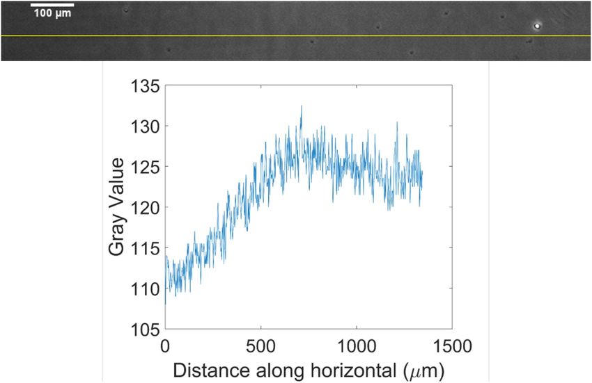
J. Phys. D: Appl. Phys. 53 (2020) 424002 S Gilbert et al
absolute black and 255 absolute white. The objective of image the image from one side of the image to the other. We consider
processing is to prepare an image for analysis, in our case by a technique described by Russ [8] using an averaging kernel
obtaining a binary image that identifies exactly the regions of operation with an array of large dimensions followed by image
interest (ROI). A binary image here is one where we assign arithmetic.
pixels part of the ROI with a value of 1, and other pixels with The averaging filter is an iterative application of a kernel
a value of 0. For images with more than one type of ROI, operation. The kernel operation is usually a square array of
multiple binary images are created and organised into chan- dimension (2 m+1)×(2n + 1), so that there is a central pixel,
nels for the respective ROI. To convert our image into the with each cell containing an integer weight. The array is put
desired form, we must first pass our matrix under a series of over an initial pixel at its centre. The centre and neighbouring
transformations to reduce noise and to accurately identify the pixels are then multiplied by the weight overlaying it. The res-
pixels truly part of a ROI. These algorithms of transformation ult is summed and divided by the sum of the weights to fit the
broadly fit under three classes: pre-processing, segmentation same 8-bit scale. This is then put as the value of the central
and post-processing. For each we will identify the obstacles in pixel in the output image. This is repeated for every pixel in
the acquired data; then explain the techniques used to resolve the input image. This can be expressed for an input image f,
them. transformed to g by the kernel ω of dimension a × b as:
Figure 1 shows a typical image used in this investigation.
This image is obtained from a co-culture system where peri-
pheral blood mononuclear cells (PBMCs) and platelets flow g(x, y) = ω ∗ f(x, y) (1)
over an adhesive substrate. Note that the PBMCs which are
initially adhered appear almost perfectly spherical and very
∑a ∑b
bright, while the PBMCs in firm adhesion are comparatively b ω(s,t)f(x−s,y−t)
= s=−a
a ∑b
∑s=t=− (2)
dark with highly heterogeneous shape. Because of these dif- −a t=−b ω(s,t)
ferences, the stages of the cell are often referred to as phase
for all pixels (x, y) in f.
bright and phase dark for initial adhesion and firm adhesion,
For pixels close to the boundary the array will extend out-
respectively.
side the perimeter of the image. To account for this a simple
method is to mirror the pixels from the boundary up to the 2
2.1. Pre-processing m pixel in the horizontal and the 2n pixel in the vertical as
padding around the image.
Pre-processing uses routines to convert raw, heterogeneous
The techniques described by Russ is to take the average of a
images into a set of standardised images with as few unwanted
large area of the image, so that extreme intensities from indi-
artefacts and accentuate features for separation in segmenta-
vidual ROIs do not skew the kernel operation, this is known
tion. The techniques of PCM do introduce certain artefacts in
as the Mean kernel. However, the area cannot be too large so
an image which could be incorrectly identified as a ROI. Dur-
that the overall differences in illumination are not lost in the
ing this stage we consider techniques that are used to normalise
output. The array of weights in ω need all pixels in the array
image-to-image brightness and account uneven illumination,
to have an equal contribution, so for a 3 × 3 region we have:
which images like figure 1 and figure 2 contain.
1 1 1
Image-to-image brightness heterogeneity. To begin eradic- ω = 1 1 1 . (3)
ating the various artefacts in the image, we first normalise 1 1 1
the pixel values so later processing techniques are repeatable
By applying a similar array with larger dimensions, fitting
across images captured with varying illumination. The average
the properties as mentioned before, results in an output show-
pixel intensity across a set of images, in our case sampled from
ing the changes in the background illumination. Then, the ori-
the training set, and the individual difference in mean pixel
ginal image is divided by this background to account for the
intensity in each subsequent image is corrected by adding the
illumination across the image.
difference to every pixel in an image so that the mean becomes
that of the set. This works well for images that are considered
reasonably similar. However, an image with a high proportion 2.2. Segmentation
of ROIs which are either really bright or really dark will skew
Segmentation is the identification of pixels as either associ-
the set’s mean. This drawback could reduce the range of the
ated with a ROI or not. The segmentation process works most
pixel intensities in other images as negative values are made
efficiently on images which have had noise and other imper-
equal to 0 and those over 255 reduced to the maximum and
fections removed to allow for the most accurate separation of
so previous variations in pixel intensity are lost, which is also
pixels to be categorised. Techniques for this stage may differ
known as contrast.
in three key areas: detection efficiency, user-operability and
computational cost. The first of these relates to the success in
Uneven image illumination. Now, we address the uneven illu- correctly identifying the ROI. The second relates to the amount
mination of the image and the ways to account for it. We can of user knowledge needed in being able to use the routine. The
observe in figure 2 that there exists an uneven illumination of last analyses the time taken to execute once the program is
3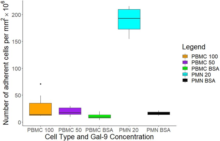
J. Phys. D: Appl. Phys. 53 (2020) 424002                                                                                          S Gilbert et al

Figure 1. A cropped area of a representative image that can be analysed through our workflow. The image shows co-cultures with
peripheral blood mononuclear cells (PBMCs) and platelets on adhesive substrates, where the PBMCs and platelets appear in different
adhesive states. The image has been labelled with a number of key features identified. First, the cells we are identifying are considered to be
at two different phases of adhesion, rolling adhesion (red) and firm adhesion (blue). Moreover, cells may be in a transition state between
these two phases (green). All cells produce the characteristic ‘halo’ as an emanating set of bright pixels surrounding the cell. However,
sometimes the ‘halo’ effect is overcompensated and can cause a following darkness in pixels (green arrow). The uneven illumination is not
obvious in this image but is normally more prominent, such as in figure 2. Irregular objects in the image are also pointed out with arrows.
The orange arrows identify platelets adhered to the surface. The magenta arrow identifies a disruption in the coating of the protein causing a
significant phase delay similar to a halo.

running. These were the properties considered when design-                resolve this problem as they depend on the type of image histo-
ing this automated workflow. We first describe the alternative            grams produced after pre-processing [16–18]. These have then
techniques considered for this methodology before describing              been integrated into workflows to form some of the current
the active learning segmentation used in the final methodo-               techniques used for segmentation, known here as automated
logy.                                                                     thresholding workflows.

Thresholding.    A key component of segmentation is                       Automated thresholding workflows.       Usually a single or mul-
thresholding. Thresholding involves an input of minimum                   tiple threshold value is unable to differentiate between ROI
or maximum pixel intensities which a ROI has been identified              and other artefacts that may have pixels of similar intensity.
to have. If the information for setting such limits is known,             Therefore, other techniques are used to utilise common fea-
then the process is simple: pixel-by-pixel, an if-statement               tures in a set of images to aid the classification of a true ROI.
transforms an 8-bit image to a binary image with the pixels                   Two very common effects in phase contrast images are
part of the ROI as 1 and the rest 0. However, in many cases the           the characteristic ‘halo’ corresponding to the refractive index
best thresholds to choose are unknown, or they are required to            and thickness values between the cell and the surrounding
be automated. There are many published algorithms that try to             medium.

                                                                      4
J. Phys. D: Appl. Phys. 53 (2020) 424002                                                                                        S Gilbert et al

Figure 2. A cropped area taken from another representative image with the values of the pixels plotted against the path across the width of
the image (yellow). Here we can see an uneven illumination from a light source, where the background illumination decreases in brightness
the further left we go.

    The halo effect is exploited in the work of Selinummi                constituent parts of images not originally trained upon. The
et al [19] and Flight et al [20] in dense colonies of epithelial         constituent parts are the different types of ROI mentioned
cells. The intuition behind both techniques is by applying a             before, and are referred to as classes in classification. The pro-
Gaussian blur or Mean kernel operation for a variety of differ-          cess can be applied in our workflow by creating a classifier
ent dimensions and then monitor the variation in pixel intens-           from a random sample of the data and then using it during our
ities. When the blur is applied, the halos are already close to          segmentation step to identify the different classes of ROIs in
maximum pixel intensity so do not vary but the darker region             the rest of the images.
of the epithelial cell quickly become brighter as the surround-              There are many active learning software tools for seg-
ing halo encroaches on the ROI. Therefore, the image is trans-           mentation already available in the bio-imaging community
formed to one with higher pixel intensity representing higher            [3, 4]. The majority of these use an algorithm called a random
variations. A subsequent application of Otsu thresholding [16]           decision forest as the foundation for the classifier [22]. This is
determines the threshold value to separate the halo, and thus            whereby a multitude of decision trees are constructed during
background, from the ROI. This was combined with fluores-                training. Then, when applied to a new object to classify, the
cent dyes identifying constituent parts of the ROI, such as the          output class is the modal class from all of the decision trees.
nucleus, and discrete mereotopology to validate the segmen-                  Ilastik is one such interactive learning and segmenta-
ted area as a ROI [21]. However, the dependency on densely               tion toolkit [23]. The Pixel Classification module calculates
packed cell colonies made these techniques unsuitable for the            35 classification features from an image matrix to interpret
images captured here.                                                    information about intensity, edge, texture and orientation.
                                                                         These help produce a classifier to be applied to other images
                                                                         to provide a prediction of the designated class for every pixel.
Active learning segmentation.     Active learning is a type of           Adjacent pixels of the same class then form our ROIs. So,
machine learning method where a user iteratively adds train-             unlike before, we are able to train the classifier to the kinds
ing data to a supervised learning algorithm until the desired            of images specifically collected with our research. In addition,
classification is achieved. In image analysis, a classifier is a         the user-friendly graphical user interface (GUI) is well-suited
set of rules based on active learning methods to identify the            for easy operation and limited user knowledge. Finally, there is

                                                                     5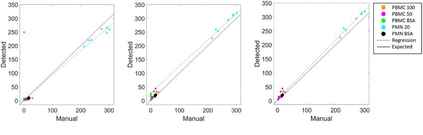
J. Phys. D: Appl. Phys. 53 (2020) 424002                                                                                         S Gilbert et al

some additional computational cost with the added complexity             data, however the technique is useful to to display the most sig-
of the algorithm although this was still significantly faster than       nificant contributions to the variability for a user to interpret.
the current manual approach, mentioned later in the results.             The relationship between variance and information is that, the
                                                                         larger the variance carried along the axis, the larger the dis-
                                                                         persion of the data points along it. Therefore, if the dispersion
2.3. Post-processing
                                                                         in that dimension is larger, the particles are more likely distin-
Post-processing describes the type of techniques used to sieve           guishable.
through a binary image produced by segmentation to remove
ROI that are in fact irregular particles. An example are the
platelets pointed out in figure 1. These cells could be detected         k-means clustering.      The k-means clustering algorithm
as smaller versions of cells as they undergo respective stages of        divides the data set into k different clusters of data-points
adhesion albeit on a smaller scale. Such techniques range from           that are considered close to each other. First, each ROI is
counting only those ROIs that are above a minimum and/or                 represented by a vector with each entry corresponding to the
maximum number of pixels to machine learning algorithms                  value of a feature. The algorithm works by initialising k differ-
separating unusual artefacts by measuring multiple morpholo-             ent centroids to some ROI. Afterwards, the algorithm assigns
gical features. In our final workflow, a minimum and/or max-             each ROI to the cluster with minimal Euclidean distance in
imum threshold for the number of pixels in a ROI is set as the           the feature space to the centroid of that cluster. Then, each
method used in post-processing. This is because the cells being          centroid µi is updated to the ROI closest to the mean of all
identified follow fairly homogeneous measurements in size                the training examples assigned to cluster i. The algorithm
for the adhered area or are significantly distinct from particles        alternates between the two steps until convergence or the
other than that being considered.                                        maximum number of iterations is achieved. The methodology
                                                                         is explained in more detail by Lloyd [26].

2.4. Analysis
                                                                         Statistical testing and inference.       In our investigation, we
We now demonstrate the effectiveness of our approach by ana-             are looking to classify the morphology of the cells of firmly
lysing images with adherent cells. We first quantify the num-            adhered cells depending on the different concentrations of
ber of cells depending on their adhesion status. This is done for        molecules. Therefore, using the null hypothesis that groupings
different experimental conditions; e.g. by varying concentra-            are independent of the molecule we are investigating, we can
tions of molecules that are suspected to affect cell adhesion.           test the statistical significance of the outcome in the analysis. If
Afterwards, we utilise a by-product of the automated work-               proven significantly different, then the shape descriptors con-
flow and begin to quantify the morphology of the cells at the            tributing the most to the principal components from the PCA
different experimental conditions.                                       indicate the features most effected by these differences.
   As the images are segmented pixel-by-pixel, to whether a
pixel belongs to the ROI or not, we have a representation of
the adhered surface area of each cell. As seen in figure 1, dur-         2.5. Validation
ing initial adhesion the cell remains in a highly circular form,
however during firm adhesion the cell migrates on the sur-               The success of classification was measured by the workflow’s
face looking to pass through. The shape of the cell can also be          precision, recall and combined score of the two as described
affected by surface proteins and can therefore provide useful            by Powers [27]. This is similar to the validation process used
information about the impact of molecules on the cells. Thus,            by many publications of the area [19, 28, 29] and hence gives a
an interest is to categorise the morphology of the firm adhesion         comparative statistic between different automated workflows.
cells to investigate the effect of different levels of molecules         The statistics necessary for these calculations describe all the
in this process. We describe the machine learning techniques             possible outcomes for a classifier. These possibilities are:
used to analyse the morphology of phase dark cells.
                                                                         • true positive (TP) - correctly identifies the adhered cell of
                                                                           interest as a ROI.
Principal component analysis.     Principal component analysis           • true negative (TN) - correctly does not identify noise as a
(PCA) is a methodology to reduce the dimensionality of a data              ROI.
set in which there are a large number of interrelated variables.         • false positive (FP) - incorrectly identifies noise as an ROI.
The methodology is explained in more detail by Jolliffe [24]             • false negative (FN) - incorrectly identifies adhered cell as
or Goodfellow et al [25]. Here each ROI identified has 10 val-             not a ROI.
ues calculated from shape descriptor formulae, refer to shape
descriptor for exact formulae. The result is a representation               Classification precision (p), or positive predictive value,
whose elements have no linear correlation with each other.               indicates the fraction of objects correctly classified as a ROI
The order depends on the variance in that dimension. The rep-            out of the total number detected, and is calculated as:
resentations, called principal components, provide a summary
ordering the most influential factors in describing morphology.                                           TP
Here it was reasonable to not reduce the dimensionality of the                                     p=           .                          (4)
                                                                                                        TP + FP
                                                                     6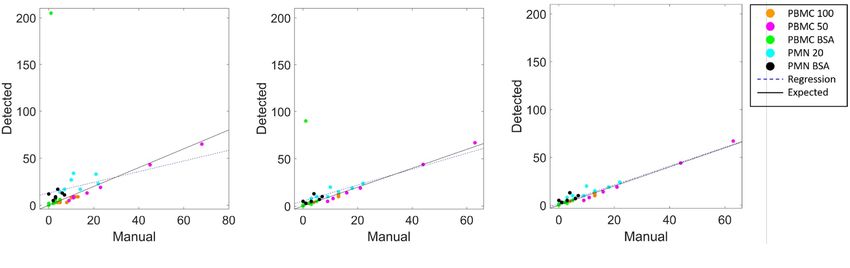
J. Phys. D: Appl. Phys. 53 (2020) 424002                                                                                         S Gilbert et al

   Classification recall (r), or sensitivity, indicates the fraction       ICAM-1 experiments.       A flow chamber assay was used to
of objects correctly classified as a ROI out of all adhered cells,         investigate the adhesion behaviour of purified PMNs on
and is calculated as:                                                      ICAM-1 under physiological flow conditions.
                                                                               Channels in an Ibidi chamber were coated with 10 µg/ml
                                    TP                                     ICAM-1-Fc. During the experiment, the isolated PMNs were
                             r=           .                     (5)
                                  TP + FN                                  perfused through the channels at a concentration of 1 × 10⁶
                                                                           in PBS containing Ca2 + and Mg2 + . PMNs were allowed to
   The proportions for r and p are expressed as percentages.               enter the chamber and then flow was suspended for 5 mins to
The F 1 score is the harmonic mean of precision and recall:                allow adhesion of cells to ICAM-1-Fc. Flow was then restarted
                                                                           at a wall shear stress of 0.1 Pa, which was applied throughout
                                    (       )                              the perfusion to mimic physiological conditions.
                                         pr
                           F1 = 2             .                 (6)            After the wash out period, a series of images was taken
                                        p+r
                                                                           under continuous flow across the channel. The total cell num-
                                                                           ber adhered was calculated from the series of images.
    An F 1 score of 0 indicates no agreement for the automated
and manual analysis, while 1 indicates complete agreement.
The final F 1 score, precision and recall is calculated as the             vWF experiments.     A flow chamber assay was used to meas-
average of the scores from both phases. Next we investigate                ure adhesion of platelets to the vMF under physiological flow
where the automated workflow can be improved with image-                   conditions.
by-image comparisons of the manual and automated number                        Glass microslides were coated with 0.1 mg/ml vWF and
of ROI. We can categorise the incorrect detection of adhered               blocked using PBS containing 2% BSA. During the experi-
cells into four categories: missing, noise, merged and split.              ment, a flow rate of 0.8 ml/min was maintained to give the
Missing describes those cells that are not detected by CASTLE              desired wall shear stress of 0.1 Pa. Anti-coagulated human
but counted by a human expert. Noise are the particles identi-             whole blood was perfused for 2 minutes over vWF. The
fied as a ROI by the automated workflow but are not counted by             microslides were then washed with PBS 0.1% BSA with or
the expert. Merged detections are the number of adhered cells              without 30 µmol/l ADP, a platelet activating agent.
that are counted as being part of another detected ROI. Finally,               After the wash out period, a series of images and videos
a split observation is a single adhered cell that is detected as           were taken under continuous flow across the microslide. Plate-
two distinct ROIs.                                                         let coverage was calculated as the number of cells adhered.
                                                                           Phase bright platelets were classed as initially adhered plate-
                                                                           lets and phase dark platelets were classed as activated platelets.
2.6. Image acquisition

Here we describe briefly the specific experiments performed                2.7. Image processing and analysis using CASTLE
to acquire the images used to validate our workflow.
                                                                           The automated workflow is visualised in figure S1 (see
                                                                           supplementary material, available online at (stacks.iop.org/
Blood sample collection. Blood samples were obtained from                  JPD/53/424002/mmedia)). The batch processing was designed
donations of volunteers who have given written informed                    as a script in the ImageJ Macro language and implemented
consent. Approval was obtained from the University of                      as a plugin in Fiji is Just ImageJ 2.0.0 [30]. The Mean and
Birmingham or Queen Mary University of London Local Eth-                   Image Calculator plugins were used in Pre-processing [31].
ics Review Committee.                                                      Training of the classifier and segmentation was carried out
                                                                           using Ilastik 1.3.2post2 [23]. Post-processing and data collec-
                                                                           tion for analysis were completed using the Analyse Particles...
Gal-9 experiments.    A flow chamber assay was used to
                                                                           plugin [31]. Analysis was carried out in R 3.6.1. [32]. The
investigate the adhesion behaviour of PBMCs and purified
                                                                           final automated workflow is available as a collection of open-
PMNs for different amounts of Gal-9 under physiological flow
                                                                           source plugins on the Cell Adhesion with Supervised Training
conditions.
                                                                           and Learning Environment (CASTLE) GitLab project, refer
   Channels in an Ibidi chamber were coated with either 20,
                                                                           to section 5. The computer used in the implementation of the
50 or 100 µg/ml Gal-9 or 1.5 % bovine serum albumin (BSA)
                                                                           CASTLE plugins had an Intel(R) Core(TM) i7-9850 H CPU
in Phosphate-buffered saline (PBS) as the control. During
                                                                           at 2.60GHz with 16GB RAM.
the experiment, the isolated PBMCs or PMNs were perfused
through the channels at a concentration of 1 × 10⁶ in PBS con-
taining Ca2 + and Mg2 + for 4 min before a wash out period                 3. Results
of 1 min. A shear wall stress of 0.1 Pa was applied throughout
the perfusion to mimic physiological conditions.                           We now apply our workflow to several data sets. We focus
   After the wash out period, a series of images was taken                 most of our discussion to the analysis of PMNs and PBMCs
under continuous flow across the channel. The cell number                  depending on concentrations of Gal-9, since these data sets
adhered per mm2 and per 1 × 10⁶ cells was calculated from                  are the most challenging to the algorithms and involve
the series of images.                                                      different cell types with quantitatively varying concentrations

                                                                       7
J. Phys. D: Appl. Phys. 53 (2020) 424002 S Gilbert et al
of molecules. We then demonstrate that our workflow can sim- Similar analysis for the validation of CASTLE was carried
ilarly be applied to the same cell types stimulated with other out on the other studies, one on leukocytes exposed to the pro-
molecules (here, ICAM-1), or very different cell types (here, tein ICAM-1 and another on platelets exposed to the protein
platelets). vWF. The final F 1 score was 87.0% and 80.7%, respectively.
Similar observations were made to that already discussed (see
tables S2, S3 and figures S3, S4). This time the iterations
of training were carried out to demonstrate the application
3.1. Validation of workflow
of CASTLE. First, we validated how CASTLE processed the
Validation of cell count. The automated workflow, CASTLE, images using the final training used in the study of the role of
was applied to the images from an ongoing study of the role of the protein Gal-9 on leukocyte adhesion. Then, we validated
the protein Gal-9 on leukocyte adhesion. For each of the five how CASTLE processed the images with an additional image
different levels of protein exposure, we obtained a sample of from the new data set, respectively. The rationale was to show
seven different images. One image from each protein expos- how CASTLE may be applied to new data sets: by adding to
ure was chosen for the classifier to be trained upon. After the the original data set of a similar study. The result is a more
automated workflow was applied, the plugin took under 11 thorough training due to more images identifying the variabil-
minutes for all 35 images to be processed (see table S1). One ity in cell appearance yet not at the expense of the researcher’s
image was excluded from the validation after statistical ana- time, who would have otherwise trained the data themselves.
lysis identified the image as an anomaly compared to similar
images of the same protein exposure (see figure S2). The final
F 1 score was 87.0%, with a 81.2% classification precision and Comparison to other methods. To confirm that the perform-
an 93.7% classification recall. ance of CASTLE was an improvement to other available work-
The final validation scores were the result of introducing flows, we compared the software to a comparable plugin in
a third ROI for classification. This was identified in figure 1 ImageJ/Fiji. The plugin is called Trainable WEKA Segment-
as a cell transitioning from initial adhesion to firm adhesion, ation (TWS) [33] and forms part of the Waikato Environment
which in manual counts were associated with the latter but for Knowledge Analysis (WEKA) collection for data mining
were considered still too bright in the automated workflow. with open-source machine learning tools [34]. Using the same
Before the new class was introduced, the F 1 score was 86.2% pre-processing and post-processing techniques as CASTLE on
with a classification precision of 89.9% and a classification the same 35 images, TWS produced a final F 1 score of 63%
recall of 82.8%. with 48% precision and 95% recall (see table S1). TWS iden-
Besides the increase in F 1 score for the count, the introduc- tified a similar number of correct cells as CASTLE. How-
tion of the new class was preferred as the following analysis ever, for this data set, TWS seemed to mis-identify as many
into morphology depended on correctly identifying all of the objects which increased the final number detected by about
cell that forms its shape. Using the same classifiers, a valida- twice as many for both phases of cell (see figure S5). Also,
tion on all the classified pixels was carried out on a sample of the time to run TWS to batch process all 35 images took 6
five images, one from each of the different cell type and pro- times longer than the comparable application by CASTLE (see
tein exposures. The five images were segmented manually by table S1). Therefore, the CASTLE workflow would appear to
an expert to identify the phase dark cells. The same five images be an improvement in accuracy and speed than what is cur-
were processed by CASTLE. The images were then compared rently available.
pixel-by-pixel. Before the introduction of the transition class
during training, the F 1 score was 69.6% with a classification
precision of 85.0% and a classification recall of 59.0%. The Distinguishing cells types and experimental conditions. In
F 1 score remained similar at 69.3% but with a higher classi- addition to the total count across all of the images, an investig-
fication precision of 89.2%, the outcome preferred, and a clas- ation into the performance of the program for the full range of
sification recall of 56.7% . cells in a particular image is presented in figures 4 and 5. These
Figure 3 shows the analysis carried out on the perform- plots display the number of cells counted manually against
ance of the automated workflow compared to that counted those detected by CASTLE. A line of least square regression is
by an expert. A perfect identification of the number of cells drawn to predict the program’s performance across the range
would result in the percentage of correctly identified cells in of cell numbers in comparison to another line for what would
the respective phases equal to 100% of the true count. We be considered a perfect count, where the detected number of
see across the phases of cells identified that the majority of cells equal those identified by the expert.
incorrect counts are due to noise and missed cells. Noise adds Figure 4 is the series of least regression plots when compar-
to the total count by leading to false positives, while missed ing the performance of CASTLE to a manual analysis when
cells reduce the final count. Figure 3(a) confirms that the intro- confronted with the images of our study for phase bright leuk-
duction of a class for transitioning cells significantly reduces ocytes. Figure 4(a) is the phase bright analysis for all of the
the number of incorrectly classified cells (i.e. improving the images when CASTLE is trained without a transition class.
precision) and the number of cells missed (i.e improving the However, the performance of the program was seen to still
recall) compared to the classification based on two classes in be detecting more cells which would be considered as trans-
figure 3(b). itioning from phase bright to phase dark, which an expert
8J. Phys. D: Appl. Phys. 53 (2020) 424002 S Gilbert et al
Figure 3. Validation of the automated workflow against manually counted and verified results from the study into the role of the protein
Gal-9 on leukocyte adhesion. (a) CASTLE validation with no transition class during training. (b) CASTLE validation with a transition class
during training. One image from both analyses was excluded after being identified as anomalous. The stacked bar chart shows, of all the
manually counted cells, how the automated workflow performed, including how mis-identified cells of the automated workflow effected
performance as a percentage of the true number of cells.
(
a) (
b) (
c)
Figure 4. Comparison of automatic to manual detection of adherent phase bright cells for each image in the study into the role of the
protein Gal-9 on leukocyte adhesion. (a) CASTLE validation with no transition class during training. (b) CASTLE validation with a
transition class during training. (c) CASTLE validation with transition class during training and the anomalous image removed from
analysis. The regression line (blue, dashed) shows a prediction for the detected counts across the range of cells in any one image. The line of
perfect agreement (black, solid) is the desired outcome with the manual count equal to the automatic count.
would consider as phase dark in their counts. After introdu- (see figure S2). After excluding the anomalous images from
cing a Transition class in the training, we see in figure 4(b) an the input data we produce the results in figure 4(c). There-
improvement in the accuracy reflected by the closer alignment fore, with the introduction of a new training class and the
of the regression line to the line representing a perfect count. exclusion of the anomalous image the final performance across
Nonetheless, we can see that an image with PBMCs exposed the different cell types and their respective protein exposures
to the control protein BSA has a significantly larger number produced a significant improvement in the correct number of
of cells detected in comparison to the other six images of the detected cells.
same experiment. On investigation of this group of images, Figure 5 is the series of least regression plot for com-
an image appeared to have many irregular particles seemingly paring the performance of CASTLE to a manual analysis
trapped under the surface of the protein which induced enough when confronted with images from our study for phase dark
of a phase difference to create the ‘halo’ effect of adhered cells leukocytes. Figure 5(a) shows the performance when both the
9J. Phys. D: Appl. Phys. 53 (2020) 424002 S Gilbert et al
(
a) (
b) (
c)
Figure 5. Comparison of automatic to manual detection of adherent phase dark cells for each image in the study into the role of the protein
Gal-9 on leukocyte adhesion. (a) CASTLE validation with no transition class during training. (b) CASTLE validation with a transition class
during training. (c) CASTLE validation with transition class during training and the series of PBMC BSA images removed from analysis.
The regression line (blue, dashed) shows a prediction for the detected counts across the range of cells in any one image. The line of perfect
agreement (black, solid) is the desired outcome with the manual count equal to the automatic count.
Transition class is yet to be introduced to the training and adhesion. We now present the analysis performed by
before the images of PBMCs exposed to BSA were analysed CASTLE. This is to demonstrate the ability of the program
for anomalies. The regression line indicates that CASTLE to process images into information easily interpreted by a
was for the majority of images accurate but diverges to under- researcher. The result is a comparison between the protein
estimate the counts for ever larger numbers of cells. Then, exposures within each cell type. This was carried out in the
the transition class was introduced into the training and the form of a student’s t-test, where the sample variance was
performance across the images is shown in figure 5(b). Here assumed to be unequal for each series of images. This was an
we are unable to observe the point representing the anomalous assumption made in the analysis and any future use of the R
image mentioned before as the 521 detected exceeds the limits script provided on the GitLab project (see section 5) allows
of the axes, the axes chosen to focus on comparing regression the use of images assumed to have an equal variance.
lines between each stage (for the inclusion of the anomalous Our primary goal was to investigate the role of Gal-9 on
image, see figure S6). The regression line here shows the trend the adhesion of PBMCs and PMNs. Table S4 displays the
of CASTLE consistently over-estimating the number of detec- results from the Student’s t-test for each pairwise compar-
ted cells. In addition to identifying the anomalous image, after ison of protein exposures between similar cells. At the 99%
further investigation, all the images with PBMCs exposed to confidence level, we can conclude that for PBMCs there is
the protein BSA were found to have no phase dark cells and so a statistically significant effect on adhesion when a surface
were subsequently excluded from further analysis using phase is coated with either 50 or 100µg/ml of Gal-9 compared to
dark cells. Using this knowledge, figure 5(c) shows the final the control. There is no statistically significant difference in
comparison after excluding these images. We know from our adhesion between 50 or 100µg/ml Gal-9 applied, at either the
earlier validation that this final iteration is an improvement in 99% or 95% confidence level. For PMN, the difference in
F 1 score from the first. For larger numbers of adhered cells in cell adhesion between 20µg/ml of Gal-9 compared to the con-
an image, the regression line is above rather than below the trol is considered statistically significant at the 99% confid-
line of perfect count. However, in the final iteration, larger ence level. Figure 6 is a visual representation of these differ-
values detected do not exceed more than 14% of the manual ences between protein exposure and their effect on the num-
count, unlike the 16% from before, and thus represent a lower ber of adhered cells per mm2 per 106 cells flown through the
proportion of additions and reason for improvement from the chamber.
first iteration. A secondary outcome of the research was to discern
whether more cells were remaining in a state of initial adhe-
sion or whether they would form a firm adhesion in the period
3.2. Effect of galectin-9 on leukocyte adhesion
between perfusion and when the images were taken.
We now demonstrate how our workflow can lead to new bio- First, we consider table S5 which displays the results of
logical insights by further analysis of the segmented images the student’s t-test for cells during initial adhesion, known as
from the data set investigating the effect of Gal-9 on leuko- phase bright cells. We are able to conclude, at the 95% con-
cyte adhesion. fidence level, that there is a statistically significant difference
between the mean number of phase bright cells when exposed
to Gal-9 compared to the control. However, the difference at
Count.The purpose of the data that we analysed with either the 99% or 95% confidence level is not considered stat-
CASTLE was to determine the effects of Gal-9 on cell istically significant for distinct levels of Gal-9. For PMN, the
10J. Phys. D: Appl. Phys. 53 (2020) 424002 S Gilbert et al
Figure 6. Boxplot for the total number of cells adhered per mm2 × 106 from the sample of seven images taken for each protein exposure.
This excludes the previously discovered anomalous image from the PBMC BSA group (see figure S2).
difference in phase bright occurrence for 20µg/ml of Gal-9 Table 1. Results of the k-means clustering on all 2496 phase dark
compared to the control is also not considered statistically sig- cells detected by CASTLE. The values represent the proportion of
cells compared to all phase dark cells detected. We then compare to
nificant at the 99% or 95% confidence levels. the number of each cell type and their exposure to the subsequent
Second, we compare the number of firmly adhered cells, clusters that cells with similar morphological features have.
known as phase dark cells, between similar cells that have
been exposed to the different levels of Gal-9. Table S6 displays Cluster 1 Cluster 2 Cluster 3 Cluster 4
the results of the Student’s t-test for each combination of pair- PBMC 50 0.028 0 0.002 1 0.004 2 0.010 2
wise comparisons. For PBMCs, we can conclude at the 99% PBMC 100 0.028 5 0.006 3 0.008 0 0.028 5
confidence level that there is a statistically significant differ- PMN 20 0.078 7 0.212 7 0.287 6 0.254 0
ence in the number of adhered cells that are phase dark when PMN BSA 0.016 5 0.00 127 0.011 9 0.020 8
Gal-9 is present on the surface at both levels. On the other
hand, the number of phase dark cells between the two amounts
of Gal-9 were considered not to be statistically significant at
either the 99% or 95% confidence level. For PMNs, the num-
ber of adhered cells that were phase dark when 20 µg/ml Gal-9 Morphology: The final analysis for the series of images is
was applied, is considered statistically significant at the 99% the shape of the adhered area between the cell and the surface
confidence level. coated in the protein. The following are the results from this
Figure S7 allows us to visualise the differences in the total analysis.
number of adhered cells detected for each protein exposure, Table 1 displays the categorisation of the cell morphology
with the number of phase bright and phase dark cells that across all protein exposures for each type of cell. First, observe
contribute to the total shown. Here we can see the different that the series of images taken for PBMC cells exposed to the
effects that Gal-9 appears to have on the differing cell types. control protein are not present. Similar to before, after invest-
For PBMCs, the Gal-9 appears to have the largest effect on the igating the anomalous image it was seen that the correspond-
number of phase bright cells detected in the image compared ing series of images contained no phase dark cells. Therefore,
to PMNs having an enormous increase in the number of phase none are in this analysis. Next, the k-means clustering was per-
dark cells. formed on four groups and so k = 4 in this analysis. Consider
the row reflecting on the categorisation of phase dark PMN
11J. Phys. D: Appl. Phys. 53 (2020) 424002 S Gilbert et al
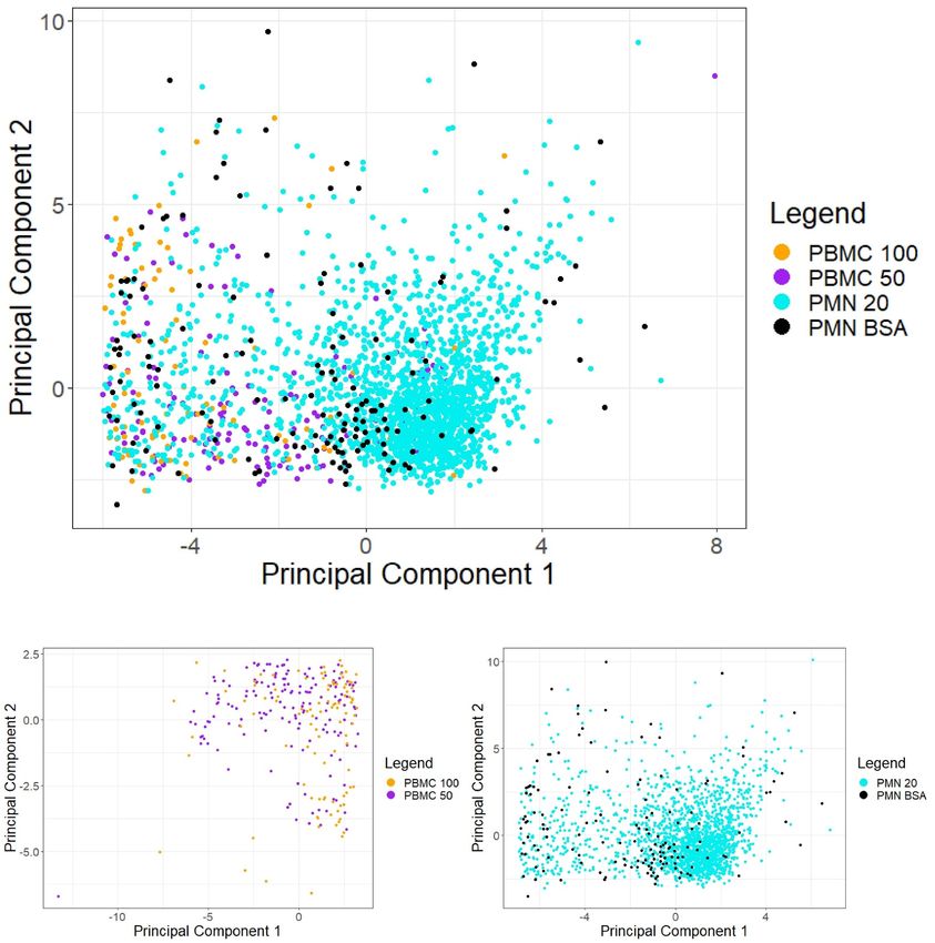
Figure 7. Morphology of adhered cells considered phase dark by CASTLE plotted in the first and second principal components for each of
the PCAs. (a) All types of phase dark cells detected in the study. The first two principal components capture 73.27% of the total variation in
cell morphology. (b) PBMC type cells only. The first two principal components capture 76.39% of the total variation in PBMC morphology.
(c) PMN type cells only. The first two principal components capture 72.13% of the total variation in PMN morphology.
cells exposed to 20µg/ml of Gal-9 to observe how well the k- into the 4th cluster. This suggests that there may be similarit-
means clustering has been able to separate the cells depending ies within each of the different cell types which are interfering
on their morphology. We see that out of the phase dark leuko- with the heterogeneity between protein exposures. Two more
cytes detected, the majority are split evenly between the 2nd, k-means clustering analyses were carried out considering only
3rd and 4th cluster. This suggests that the k-means clustering the same type of phase dark cells.
was unable to differentiate the morphology compared to the Table 2 shows the analysis in morphology of the PBMC
other cells and protein exposures. However, the majority of the cells exposed to the different levels of Gal-9. The first obser-
detected PMN cells exposed to the control were also grouped vation is the relatively even distribution of cells between both
12J. Phys. D: Appl. Phys. 53 (2020) 424002 S Gilbert et al
Table 2. Results of the k-means clustering on the 298 phase dark Figure 7(b) is a PCA on PBMCs only. We observe that
PBMCs detected by CASTLE. The values represent the proportion although both groups of Gal-9 exposure have values distrib-
of cells compared to the number of phase dark PBMCs detected. We
then compare to the number of each cell type and their exposure to
uted across the range of first and second principal component
the subsequent clusters that cells with similar morphological values, that there could be some trend. This trend is in refer-
features have. ence to many of the PBMCs with 50 µg/ml are more apparent
from just lower that -5 to 2.5 in the first principal component
Cluster 1 Cluster 2
but for mainly positive values in the second component. This
PBMC 50 0.161 1 0.223 4 is compared to the more apparent regimes for PBMCs appear-
PBMC 100 0.369 9 0.245 4 ing between 0 to 2.5 in the first principal component and from
lower than -5 to 2.5. This is a result not obvious in figure 7(a)
but is more obvious with the individual analysis, most likely
due to less cell heterogeneity.
Table 3. Results of the k-means clustering on only the 2112 phase
In figure 7(c), inferences in trend can be made about the
dark PMNs detected by CASTLE. The values represent the
proportion of cells compared to the number of phase dark PMN differences from exposure to Gal-9 to the control for PMNs.
cells detected. We then compare to the number of each cell type and Many of the points are dispersed closely about (0,0). How-
their exposure to the subsequent clusters that cells with similar ever, the majority of points appear for positive values in the
morphological features have. first principal component for those exposed to Gal-9 than those
Cluster 1 Cluster 2 that do not. On the other hand, those exposed to the control,
although some begin to cluster about (-1,-1), have many val-
PMN 20 0.380 6 0.548 6 ues at the extremes of one or both of the principal compon-
PMN BSA 0.034 1 0.036 5 ents. Referring back to figure 7(a), this appears to be the case
too. This observation could suggest that instead of exposure to
Gal-9 causing new or more extreme phenotypes in the cell that
it encourages a specific morphology already possible by the
clusters for each level of protein exposure. Thus, there appears cells under normal adhesion. To understand what morphology
to be a difference in morphology within the class of phase dark a cluster represents, referring back to the shape descriptors that
cells which is more apparent than the difference caused by the contribute the most to the first and second components can
adhesion to Gal-9. identify which are less variable to exposures of Gal-9.
Table 3 is the result in the k-means clustering for phase dark
PMNs. It appears that PMN cells exposed to 20µg/ml of Gal-
3.3. Application of CASTLE to other data sets
9 is still evenly distributed between the two clusters although
those exposed to Gal-9 are more similar to the second cluster We now demonstrate the applicability of our workflow to two
than the first. However, no significant distinction can be made other studies of cell adhesion: one investigating the effect of
from this analysis. ICAM-1 on PMN adhesion, and the other investigating the
In all of the k-means clustering analyses of morphology we adhesion of platelets in dependence on vWF and ADP. The
have been unable to determine a separation of a cell’s mor- biological interpretation of these results are not discussed here,
phology depending on their protein exposure. To better under- but the results from CASTLE are reproduced in the supple-
stand this, we show the first two principal components in fig- mentary materials to show the applicability of CASTLE to dif-
ure 7. This shows the first two independent dimensions that ferent data sets. Using a similar flow assay as for the studies
capture the highest variance to help separate the data and feed into Gal-9 (see section 2.6), we quantify the number of adher-
into the k-means clustering algorithm. We choose the first two ent cells in the images from both studies.
components only as they can be easily displayed. For the first In the study introducing ICAM-1 exposure on PMNs, each
analysis, shown here as figure 7(a), the PCA is not able to sep- image was from a repeated flow assay experiment. The results
arate the data sufficiently enough to be easily distinguished produced by CASTLE are displayed in figure S8, showing the
into the different groups of cells. This seems similar to the total number of adhered cells and the proportions of which are
figures 7(b) and (c) for the PCA for PBMC and PMN cells, phase bright and phase dark.
respectively. However, these plots are still able to convey rela- In the study on platelets, an investigation into the role of
tionships between the morphology and the protein exposure. vWF in the adhesion of platelets is considered, in depend-
For example, figure 7(a) can begin to identify characteristics ence of ADP. As in the application of CASTLE to the first
between the two types of cell through their morphology. Here, study, figure S9 shows the total number of adhered cells and
we are able to see in the first principal component that PBMCs the proportions of which are phase bright and phase dark. In
appear with a negative value in the first principal component addition, as there was a dependence on ADP between images,
for all but a few points. This is in contrast to PMNs which the figure S10 shows the number of adherent platelets obtained
majority exposed to Gal-9 appear above 0 and those exposed at different time points within the same experiment with and
to the control appearing across the full range. When consider- without ADP. We observe a higher number of adherent cells
ing the second principal component, there appears to be 2 gen- in the presence of ADP. Moreover, table S7 shows that the
eral sub-classifications forming with a cluster of points centred difference in total, phase bright and phase dark adhered plate-
about (1,-1) and the rest sparsely centred about (-4,0). lets when ADP was introduced is statistically significant at the
13You can also read