Comparison of Modelling Strategies for Ground Settlements due to Groundwater Drawdown
←
→
Page content transcription
If your browser does not render page correctly, please read the page content below
Comparison of Modelling Strategies
for Ground Settlements due to
Groundwater Drawdown
Multi-criteria analysis for comparison of three software
packages
Master’s thesis in Infrastructure and Environmental Engineering

LINNEA JOHANSSON
FRIDA ÖGGER

DEPARTMENT OF ARCHITECTURE AND CIVIL ENGINEERING
C HALMERS U NIVERSITY     OF   T ECHNOLOGY
Gothenburg, Sweden 2021
www.chalmers.se
Master’s thesis 2021

Comparison of Modelling Strategies for Ground
 Settlements due to Groundwater Drawdown

Multi-criteria analysis for comparison of three software packages

                     LINNEA JOHANSSON
                        FRIDA ÖGGER

           Department of Architecture and Civil Engineering
                 Division of Geology and Geotechnics
                     Geotechnics Research Group
             Chalmers University of Technology
                      Gothenburg, Sweden 2021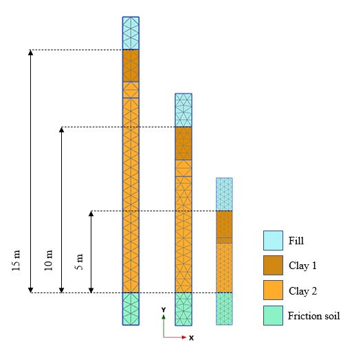
Comparison of Modelling Strategies for Ground Settlements due to Groundwater
Drawdown
Multi-criteria analysis for comparison of three software packages
LINNEA JOHANSSON
FRIDA ÖGGER

© LINNEA JOHANSSON, 2021.
© FRIDA ÖGGER, 2021.

Supervisors: Linn Ödlund Eriksson, Sweco
Ezra Haaf, Department of Architecture and Civil Engineering
Pierre Wikby, Department of Architecture and Civil Engineering
Ayman Abed, Department of Architecture and Civil Engineering
Examiner: Lars Rosén, Department of Architecture and Civil Engineering

Master’s Thesis 2021
Department of Architecture and Civil Engineering
Division of Geology and Geotechnics
Geotechnics Research Group
Chalmers University of Technology
SE-412 96 Gothenburg
Telephone +46 31 772 1000

Typeset in LATEX, template by Magnus Gustaver
Printed by Chalmers Reproservice
Gothenburg, Sweden 2021

iv
Comparison of Modelling Strategies for Ground Settlements due to Groundwater
Drawdown
Multi-criteria analysis for comparison of three software packages
LINNEA JOHANSSON
FRIDA ÖGGER
Department of Architecture and Civil Engineering
Chalmers University of Technology

Abstract
When performing construction projects below the groundwater level, groundwater
leakage into the construction can occur, which can lead to settlements. This Mas-
ter’s thesis aims at comparing three different software packages for calculation of
settlements caused by groundwater drawdown in an aquifer situated below com-
pressible soils. The different software packages used are: a stochastic settlement
model that considers creep effects and parameter uncertainties, the Soft Soil Creep
model available in Plaxis 2D and the Chalmers model with creep available in GS Set-
tlement. To evaluate the appropriateness of them, settlement calculations for both
1D and 2D soil models are performed, together with a multi-criteria analysis (MCA).

The 1D modelling results show that all three approaches exhibit the same elastic-
and elasto-plastic behaviour. For comparison of the creep behaviour between Plaxis
2D and GS Settlement, differences arise due to model formulations. GS Settlement
seems to predict lower creep settlements than Plaxis for stress states around the
preconsolidation pressure. For drawdowns that highly exceed the preconsolidation
pressure, GS Settlement instead predicts higher settlements compared to Plaxis.
The stochastic settlement model does not include creep effects, but the additional
deformation is captured by the parameter uncertainty interval for drawdowns near
the preconsolidation pressure and higher. When comparing 2D effects of consol-
idation, the ability for the stochastic settlement model to capture the additional
settlements predicted by Plaxis 2D is ambiguous.

The results in this thesis highlight the differences between the three software pack-
ages. The MCA shows that the stochastic settlement model has a good capability
in handling spatial uncertainties, but is disadvantageous due to the low level of intu-
ition. Plaxis can handle complex geometries, but the calculation is time demanding.
GS Settlement is more intuitive with lower calculation effort required, but lacks the
ability of performing calculations with complex geometries. The MCA further em-
phasises that the ability to implement the theoretical framework of a groundwater
drawdown together with modelling a drawdown over a large area is considered of
high importance. To make it less subjective, further prerequisites which define the
features of the project is needed. Hence, this comparison can serve as a support for
future projects to achieve a versatile analysis in a structured way.

Keywords: Ground settlements, Groundwater drawdown, Soft clays, Plaxis 2D, GS
Settlement, Analytical modelling, Multi-criteria analysis.

                                                                                     v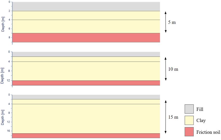
Acknowledgements
This Master’s Thesis was written at the Division of Geology and Geotechnics at
Chalmers University of Technology during the spring semester 2021.

We would like to express our sincere gratitude for the wide-spread commitment and
support during this final semester of our studies. Our thanks goes to Ezra Haaf at
Chalmers for supervising and guiding us in structuring the work. We would also like
to thank Pierre Wikby at Chalmers for his supervision and assistance at every stage
of this thesis. Our gratitude extends to our supervisor Ayman Abed at Chalmers
for his encouragement and support in the modelling process, and to Linn Ödlund
Eriksson at Sweco for her supervision in the project and guidance within the fields
of geotechnics and hydrogeology. We are further grateful for the support from our
Examiner Lars Rosén at Chalmers, who provided us with knowledge and experiences
in the multi-criteria analysis. We would likewise thank Jonas Sundell at the Swedish
Transport Administration, for his insightful suggestions in shaping our method and
results. At last, we are thankful for the valuable help from the employees at Sweco
for sharing their competences.

                                                  Linnea Johansson & Frida Ögger
                                                           Gothenburg, June 2021

                                                                                 vii
Contents
List of Figures xi
List of Tables xiii
Nomenclature xv
1 Introduction 1
1.1 Background . . . . . . . . . . . . . . . . . . . . . . . . . . . . . . . . 1
1.2 Aims and objectives . . . . . . . . . . . . . . . . . . . . . . . . . . . 2
1.3 Limitations . . . . . . . . . . . . . . . . . . . . . . . . . . . . . . . . 2
1.4 Research questions . . . . . . . . . . . . . . . . . . . . . . . . . . . . 2
2 Theoretical background 3
2.1 Groundwater conditions . . . . . . . . . . . . . . . . . . . . . . . . . 3
2.2 Stresses in soils . . . . . . . . . . . . . . . . . . . . . . . . . . . . . . 4
2.3 Consolidation and creep . . . . . . . . . . . . . . . . . . . . . . . . . 4
2.4 Influence of groundwater drawdown . . . . . . . . . . . . . . . . . . . 5
2.5 Constitutive models . . . . . . . . . . . . . . . . . . . . . . . . . . . . 6
2.5.1 Soft Soil and Soft Soil Creep model . . . . . . . . . . . . . . . 6
2.5.2 Chalmers model with and without creep . . . . . . . . . . . . 8
2.5.3 Analytical model with a probabilistic assessment of uncertainties 10
2.6 Computational tools . . . . . . . . . . . . . . . . . . . . . . . . . . . 12
2.6.1 Stochastic settlement model . . . . . . . . . . . . . . . . . . . 12
2.6.2 Plaxis 2D . . . . . . . . . . . . . . . . . . . . . . . . . . . . . 12
2.6.3 GS Settlement . . . . . . . . . . . . . . . . . . . . . . . . . . . 12
2.7 Multi-criteria analysis . . . . . . . . . . . . . . . . . . . . . . . . . . 13
3 Method 15
3.1 Case study . . . . . . . . . . . . . . . . . . . . . . . . . . . . . . . . . 15
3.2 Model setup . . . . . . . . . . . . . . . . . . . . . . . . . . . . . . . . 17
3.2.1 Stochastic settlement model . . . . . . . . . . . . . . . . . . . 19
3.2.2 Plaxis model . . . . . . . . . . . . . . . . . . . . . . . . . . . 21
3.2.3 GS model . . . . . . . . . . . . . . . . . . . . . . . . . . . . . 27
3.3 Multi-criteria analysis . . . . . . . . . . . . . . . . . . . . . . . . . . 29
4 Results 35
4.1 Modelling results of 1D cases . . . . . . . . . . . . . . . . . . . . . . 35
ixContents
4.2 Modelling results of 2D cases . . . . . . . . . . . . . . . . . . . . . . 43
4.3 Scoring of alternatives . . . . . . . . . . . . . . . . . . . . . . . . . . 44
4.4 Weighting of criteria . . . . . . . . . . . . . . . . . . . . . . . . . . . 49
4.5 Combining scores and weights . . . . . . . . . . . . . . . . . . . . . . 50
4.6 Sensitivity analysis of weighting . . . . . . . . . . . . . . . . . . . . . 50
5 Discussion 51
5.1 Modelling results . . . . . . . . . . . . . . . . . . . . . . . . . . . . . 51
5.2 Sources of error . . . . . . . . . . . . . . . . . . . . . . . . . . . . . . 53
5.3 MCA results . . . . . . . . . . . . . . . . . . . . . . . . . . . . . . . . 54
5.4 Sensitivity analysis of weighting . . . . . . . . . . . . . . . . . . . . . 55
6 Conclusions and future work 57
6.1 Conclusion . . . . . . . . . . . . . . . . . . . . . . . . . . . . . . . . . 57
6.2 Future studies . . . . . . . . . . . . . . . . . . . . . . . . . . . . . . . 58
References 59
A Modelling results I
B Weighting results III
C Normalisation of weights IX
D Combining scores and weights XI
E Alternative weighting scenarios XIII
xList of Figures
1.1 Cause-effect chain from leakage to damage (Sundell, 2018). Adapted
with permission. . . . . . . . . . . . . . . . . . . . . . . . . . . . . . . 1
2.1 Schematic model of a soil profile illustrating the upper and lower aquifer. 3
2.2 Definition of the compression and swelling index κ∗ and λ∗ (Amavasai
& Karstunen, 2017). Reprinted with permission. . . . . . . . . . . . . 7
2.3 Definition of the creep index µ∗ (Amavasai & Karstunen, 2017).
Reprinted with permission. . . . . . . . . . . . . . . . . . . . . . . . . 7
2.4 Swedish practice of modulus curve and the improved curve proposed
by Claesson (2003). Reprinted with permission. . . . . . . . . . . . . 9
2.5 The time resistance number model (Claesson, 2003). Reprinted with
permission. . . . . . . . . . . . . . . . . . . . . . . . . . . . . . . . . 9
3.1 Methodology flow chart. . . . . . . . . . . . . . . . . . . . . . . . . . 15
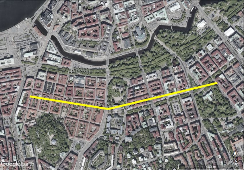
3.2 Soil type map over the Haga area in Gothenburg, Copyright SGU
(2021). . . . . . . . . . . . . . . . . . . . . . . . . . . . . . . . . . . . 16
3.3 Map over the Haga area with the chosen section. Copyright Google
Earth (2021). . . . . . . . . . . . . . . . . . . . . . . . . . . . . . . . 17
3.4 Stress chart for 5, 10 and 15 m section with different drawdown sce-
narios. . . . . . . . . . . . . . . . . . . . . . . . . . . . . . . . . . . . 18
3.5 1D models used in Plaxis. . . . . . . . . . . . . . . . . . . . . . . . . 22
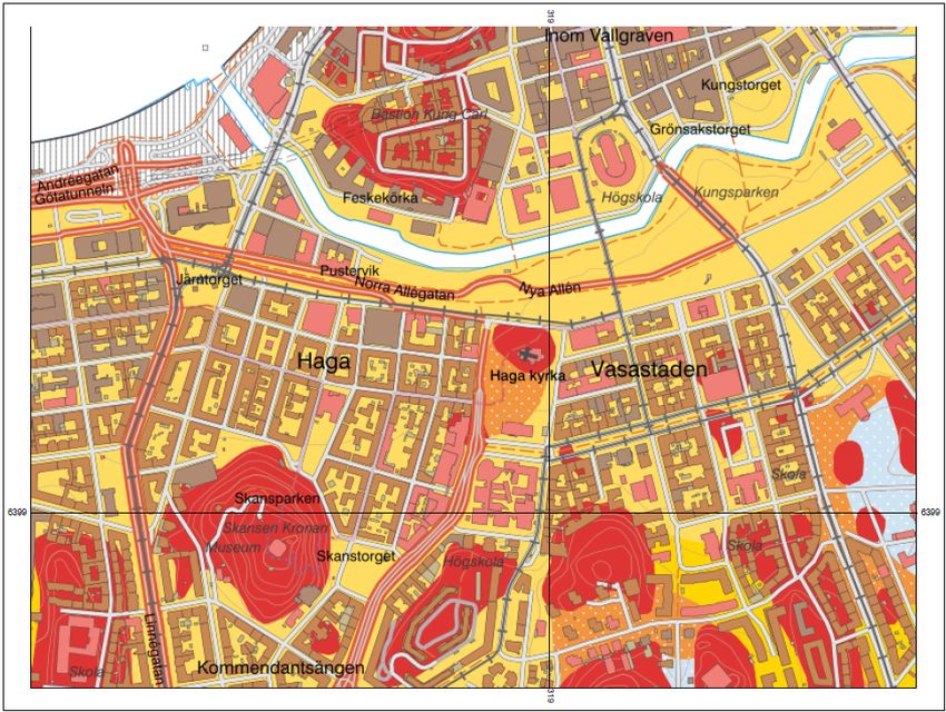
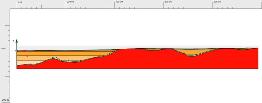
3.6 Soil stratigraphy of the chosen section in Haga. . . . . . . . . . . . . 24
3.7 Close-up of the soil stratigraphy of the chosen section in Haga. . . . . 25
3.8 GS Settlement models. . . . . . . . . . . . . . . . . . . . . . . . . . . 27
4.1 Comparison of elastic and creep model in the stochastic model, Plaxis
and GS for (a) t = 20 days, (b) t = 1 year, (c) t = 10 years. . . . . . 36
4.2 Settlement for 10 m clay and 20 kPa drawdown, without creep. . . . . 37
4.3 Excess pore pressure for 10 m clay and 20 kPa pressure decrease for
(a) Plaxis and (b) GS. . . . . . . . . . . . . . . . . . . . . . . . . . . 37
4.4 Excess pore pressure for (a) -5 kPa, (b) -20 kPa and (c) -50 kPa, for
10 m clay. . . . . . . . . . . . . . . . . . . . . . . . . . . . . . . . . . 38
4.5 Varying pressure decrease for (a) the stochastic model (50th per-
centile), (b) Plaxis and (c) GS. . . . . . . . . . . . . . . . . . . . . . 39
4.6 Comparison of 5th and 95th percentile in the stochastic model without
creep with predicted settlement in Plaxis and GS with creep for (a)
-5 kPa (b) -20 kPa and (c) -50 kPa. . . . . . . . . . . . . . . . . . . . 40
xiList of Figures
4.7 Effect of clay layer thickness for (a) stochastic model (50th percentile)
(b) Plaxis and (c) GS models subjected to 20 kPa pressure decrease. . 41
4.8 10 m clay 20 kPa drawdown, with and without upper undisturbed
zone for (a) Plaxis and (b) GS. . . . . . . . . . . . . . . . . . . . . . 41
4.9 5 m clay 50 kPa drawdown, with and without upper undisturbed zone
for (a) Plaxis and (b) GS. . . . . . . . . . . . . . . . . . . . . . . . . 42
4.10 Comparison of the settlements in the stochastic model (50th per-
centile) and Plaxis for 20 kPa drawdown and (a) 10 m clay and (b)
15 m clay. . . . . . . . . . . . . . . . . . . . . . . . . . . . . . . . . . 43
4.11 Comparison of the excess pore pressure profile for the Statistial model
and Plaxis for 20 kPa drawdown of a (a) 10 m clay and (b) 15 m clay. 44
4.12 Weights for the different criteria and sub-criteria. . . . . . . . . . . . 49
4.13 Combination of scores and weights. . . . . . . . . . . . . . . . . . . . 50
A.1 Excess pore pressure for a 10 m section and 20 kPa pressure decrease
after 1 day. . . . . . . . . . . . . . . . . . . . . . . . . . . . . . . . . I
xiiList of Tables
2.1 Basic parameters of the Soft Soil Creep model (Plaxis, 2019). . . . . . 8
2.2 Parameters of the Chalmers model without creep (Novapoint, 2021b). 10
2.3 Additional parameters for the Chalmers model with creep (Novapoint,
2021b). . . . . . . . . . . . . . . . . . . . . . . . . . . . . . . . . . . . 10
2.4 Parameters for the analytical model with a probabilistic assessment
of parameters (Larsson, Bengtsson, & Eriksson, 1997). . . . . . . . . 11
3.1 Input parameters describing the soil stratigraphy for the characteris-
tic sections in the 1D case. . . . . . . . . . . . . . . . . . . . . . . . . 19
3.2 Soil parameters used in the simulation. . . . . . . . . . . . . . . . . . 20
3.3 Input parameters describing the soil stratigraphy for three character-
istic sections in the 2D case. . . . . . . . . . . . . . . . . . . . . . . . 21
3.4 Clay 1, Soft Soil Creep model. . . . . . . . . . . . . . . . . . . . . . . 22
3.5 Clay 2, Soft Soil Creep model. . . . . . . . . . . . . . . . . . . . . . . 23
3.6 Calculation phases for 1D analysis in PLAXIS 2D. . . . . . . . . . . . 24
3.7 Clay 3, Soft Soil model. . . . . . . . . . . . . . . . . . . . . . . . . . . 25
3.8 Clay 4, Soft Soil model. . . . . . . . . . . . . . . . . . . . . . . . . . . 26
3.9 Calculation phases for 2D analysis in Plaxis. . . . . . . . . . . . . . . 26
3.10 Coordinates for the two chosen clay depths. . . . . . . . . . . . . . . 26
3.11 Clay layer 1, Chalmers with creep. . . . . . . . . . . . . . . . . . . . 27
3.12 Clay layer 2, Chalmers with creep. . . . . . . . . . . . . . . . . . . . 28
3.13 All criteria and their associated sub-criteria. . . . . . . . . . . . . . . 29
3.14 Scoring of criterion 1 . . . . . . . . . . . . . . . . . . . . . . . . . . . 32
3.15 Scoring of criterion 2 . . . . . . . . . . . . . . . . . . . . . . . . . . . 33
3.16 Scoring of criterion 3 . . . . . . . . . . . . . . . . . . . . . . . . . . . 33
3.17 Scoring of criterion 4 . . . . . . . . . . . . . . . . . . . . . . . . . . . 33
4.1 Scoring of criterion 1 . . . . . . . . . . . . . . . . . . . . . . . . . . . 45
4.2 Scoring of criterion 2 . . . . . . . . . . . . . . . . . . . . . . . . . . . 46
4.3 Scoring of criterion 3 . . . . . . . . . . . . . . . . . . . . . . . . . . . 47
4.4 Scoring of criterion 4 . . . . . . . . . . . . . . . . . . . . . . . . . . . 48
B.1 Form for weighting of criteria and sub-criteria. . . . . . . . . . . . . . III
B.2 Weighting by specialist A. . . . . . . . . . . . . . . . . . . . . . . . . IV
B.3 Weighting by specialist B. . . . . . . . . . . . . . . . . . . . . . . . . V
B.4 Weighting by specialist C. . . . . . . . . . . . . . . . . . . . . . . . . VI
B.5 Weighting by specialist D. . . . . . . . . . . . . . . . . . . . . . . . . VII
xiiiList of Tables
C.1 Normalisation of weights for criteria and sub-criteria. . . . . . . . . . IX
D.1 Combination of scores and weights. . . . . . . . . . . . . . . . . . . . XI
E.1 Combination of scores and weights for alternative scenario 1. . . . . . XIII
E.2 Combination of scores and weights for alternative scenario 2. . . . . . XIV
E.3 Combination of scores and weights for alternative scenario 3. . . . . . XV
xivNomenclature
Roman letters
a Regression parameter [-]
a0 Constant describing the improved modulus curve [-]
a1 Constant describing the improved modulus curve [-]
b Regression parameter [-]
b0 Factor < 1 [-]
b1 Factor > 1 [-]
0
cref Reference cohesion intercept [kPa]
Cc Compression index [%]
Cs Swelling index [%]
Cα Secondary compression index [%]
E Young’s modulus [kPa]
e Void ratio [-]
einit Initial void ratio [-]
hinit Location of the groundwater level for lower aquifer [m]
hnew Location of the groundwater level after lowering [m]
k Permeability [m/s]
nc
K0 Lateral earth pressure for normally consolidated soils [-]
ki Initial permeability [m/s]
M Shape parameter dependent on K0nc [-]
m0 Modulus number at stress levels above the limit stress [-]
∗
M Parameter related to the aspect ratio of the ellipsoid [-]
M0 Compression modulus for σv0 < σc0 [kN/m2 ]
ML Compression modulus for σc0 < σv0 < σL0 [kN/m2 ]
p0 Mean effective stress [kPa]
r Creep parameter [-]
2
R Coefficient of determination in statistics [-]
rs Time resistance number [-]
tref Reference time [days]
u Pore water pressure [kPa]
wn Natural water content [%]
xvNomenclature
Greek letters
αs Creep parameter or secondary compression index [-]
αs(max) Coefficient of secondary compression at the apparent
preconsolidation pressure [-]
βα s Coefficient of change in coefficient of secondary compression
with compression [-]
βk Coefficient of change in permeability with compression [-]
γ Unit weight [kN/m3 ]
γw Unit weight of water [kN/m3 ]
γsat Saturated unit weight [kN/m3 ]
γunsat Unsaturated unit weight [kN/m3 ]
κ∗ Modified swelling index [-]
λ∗ Modified compression index [-]
µ Mean value [-]
µ∗ Modified creep index [-]
0
νur Poisson’s ratio for unloading and reloading [-]
φ0 Friction angle [◦ ]
ψ Dilatation angle [◦ ]
ρ Density [kg/m3 ]
σ Standard deviation [-]
σ Total normal stress [kPa]
σ0 Effective stress [kPa]
σc0 Preconsolidation stress [kPa]
σL0 Limit effective stress where the modulus curve begins to
increase [kPa]
σv0 Effective vertical stress [kPa]
0
σvc Vertical preconsolidation stress [kPa]
σt Tensile strength [kPa]
τf u Undrained shear strength from vane test [kPa]
εp Volumetric strain [%]
xviNomenclature
Abbreviations
CRS Constant rate of strain
FEM Finite element method
MCA Multi-criteria analysis
OCR Overconsolidation ratio
SGU Geological Survey of Sweden
SS Soft Soil
SSC Soft Soil Creep
xviiNomenclature xviii
1
                             Introduction

1.1      Background
During underground construction projects, there is a risk of leakage of the ground-
water into the construction. If the construction work has to be performed in a dry
environment, the water must be pumped or prevented from leaking in. In areas
with soft soils, this might lead to settlements, which cause damages on structures
and consequently, high costs. The magnitude of a damage depends on the size and
duration of the groundwater drawdown, the geotechnical conditions and the sensi-
tivity of the damaged object (Merisalu et al., 2020). The full process of how risk of
damages arises due to leakage into underground construction is explained by Sundell
et al. (2015). The cause-effect chain is presented in Figure 1.1.

Figure 1.1: Cause-effect chain from leakage to damage (Sundell, 2018). Adapted
with permission.

To quantify the risks, it is vital to have a well-functioning tool for prediction of settle-
ments caused by changes in groundwater conditions. Today, analytical and numeri-
cal models have been extensively used in both research and by industry professionals
in Sweden to perform settlement calculations due to groundwater drawdown. Mate-
rial models and mathematical programs have been developed continuously but there
is a lack of studies that compare their appropriateness for estimating settlements
due to changes in groundwater conditions. This could potentially meet a need to
further interlink hydrogeological and geotechnical competences. Depending on the
context of the underground construction project, it possesses varying prerequisites.
This entails that different computational alternatives can be better suitable in dif-
ferent projects. To address this problem, a multi-criteria analysis together with a
comparison of settlement prediction between the alternatives can be performed to
obtain a comprehensive and structured comparison of models. This could further
serve as a support in a risk assessment framework not to underestimate the risk and
cause harm to the environment or not overestimate it and take too many precau-
tions. A more precise prediction might reduce material use, which is beneficial both
from an environmental as well as an economical point of view.

                                                                                          1
1. Introduction
1.2 Aims and objectives
The purpose of this Master’s thesis is to compare three different computational
tools based on how suitable they are in predicting settlements caused by a ground-
water drawdown in the lower aquifer. This will be achieved partly with a literature
study to clarify the basic theories for how settlements are caused by groundwater
drawdowns, partly with a multi-criteria analysis for a structured comparison of the
performance of computational tools available. The first software package that is
studied and practised is a statistical settlement model, which considers parameter
uncertainties. It is part of a risk assessment framework developed by Sundell et al.
(2019a) and has been supplemented with a creep model by Wikby and Andersson
(2020). The next two software packages are Plaxis 2D with the Soft Soil Creep
model and GS Settlement with the Chalmers with Creep model. The analysis will
be achieved by setting up representative and comparable soil models inspired by the
site characteristics of the Haga passage, which is a part of the West Link project in
Gothenburg.
1.3 Limitations
The study is limited to examine the effect of pressure change in a lower groundwater
aquifer situated below a layer of compressible soils. Furthermore, settlement is only
examined for cohesive soils in the form of clay. The deformation in the fill and
frictional soil layers situated above and below the cohesive clay soils will in this
case be considered negligible. The study covers the entire settlement process; both
consolidation and creep to best represent reality. A delimitation is made to evaluate
normal to slightly overconsolidated clays, which is typical for clays at the Swedish
west coast. The study will use a set of predefined drawdowns in the lower aquifer and
implement them in the three computational alternatives for settlement prediction.
Hence it is limited to not predict the magnitude of the drawdowns. Lastly, the
whole cause-effect chain is not considered - it only covers the parts that processes
’reduction of groundwater levels’ to ’soil subsidence’, shown in Figure 1.1.
1.4 Research questions
The following research questions are to be answered in this thesis:
• How does the pore pressure profile in the clay change when the groundwater
pressure head is lowered in the lower aquifer?
• What is required to perform modelling of groundwater induced subsidence in
the stochastic settlement model, Plaxis 2D and GS Settlement?
• How do the stochastic settlement model, Plaxis 2D and GS Settlement perform
when modelling coupled hydrogeological and geotechnical problems and how
does their appropriateness differ depending on the scenario observed?
22
Theoretical background
2.1 Groundwater conditions
Groundwater fills up voids in underground permeable materials. The upper bound
of the groundwater zone is referred to as the water table (Winter et al., 1999), and
can be detected at different levels depending on confined or unconfined conditions
(SGU, 2019). An unconfined groundwater aquifer is in direct contact with the
atmospheric pressure while confined conditions implies that the water zone is fully
saturated and overlaid by a low permeable soil layer, such as clay, called aquitard
(Carlsson & Gustafsson, 1984). The aquitard enables the confined aquifer to have a
pressure level above its upper boundary. This level is referred to as pressure head.
A conceptual model that shows a soil section with the upper and lower aquifers is
presented in Figure 2.1.
Figure 2.1: Schematic model of a soil profile illustrating the upper and lower
aquifer.
The flow of groundwater is complex due to heterogeneity of the soil structure. The
rate of flow is governed by the type of soil and its hydraulic conductivity together
with the difference in pressure head, known as the hydraulic gradient. This phe-
nomenon can be explained by Darcy’s law, where the rate of water flow through a
32. Theoretical background known medium is proportional to the difference in height of the water and inversely proportional to the length of the flow path (Fetter, 2014). 2.2 Stresses in soils A soil structure can be interpreted as a skeleton made up of solid particles that surrounds continuous voids filled with water and/or air. The volume of the soil can change because of rearrangement of the soil particles, which will lead to trans- mission of stresses between the particles. For fully saturated soils the stresses can be explained by the principle of effective stress which was introduced primarily by Terzaghi (1923). It provides a relationship by three different stresses; total normal stress σ acting on a plane, pore pressure u that fills up the voids and effective normal stress σ 0 which is the stress that represent the interparticle forces. The relationship is σ 0 = σ − u (Knappett & Craig, 2012). 2.3 Consolidation and creep The process of when a fully saturated soil with low permeability undergoes a change in volume because of change in effective stress is called consolidation. There are a plethora of studies and literature describing the way in which soft soils behave during compression and consolidation and how it can be modelled. One of many theories is the one provided by Terzaghi that encompasses a one-dimensional con- solidation process (Olsson, 2010), and is explained in more detail by for instance Knappett and Craig (2012) and Sällfors (2013). Consolidation occurs due to increase in effective stress and generation of excess pore pressure of the same magnitude as the applied load. This generation of excess pore pressure can for example be caused by a reduction of the pressure head. Over time, difference in excess pore water between different pressure zones will cause a flow of pore water in order to approach equilibrium. Subsequently, the soil will experience a compression. The compression behaviour of a soil is strongly linked to its stress history. If the present effective stress in a soil is the largest that the soil has experi- enced, it is said to be normally consolidated. An overconsolidated soil, on the other hand, has been exposed to higher stresses in the past. The term overconsolidation ratio (OCR) is used to classify whether a soil is normally consolidated or over con- solidated. It is expressed as the ratio between the maximum stress that the soil has been subjected to, known as the preconsolidation pressure, and the current stress state (Knappett & Craig, 2012). After the dissipation of the excess pore pressure there is still a possibility for the soil to deform but at a slower pace, referred to as secondary compression or creep (Sällfors, 2013). While primary consolidation is controlled by the dissipation of ex- cess pore pressure and Darcy’s law, secondary compression or creep is instead con- trolled by soil viscosity (Leroueil, 2006). It is defined as a time dependent decrease in volume during a constant stress. According to Larsson (2008) the separation 4
2. Theoretical background

of primary and secondary could be considered as imaginary, since the secondary
compression is present during primary compression as well. If the current stress
state constitutes 80 percent of the preconsolidation pressure, there is reason to con-
sider creep (Larsson, 1986). Creep is generally characterized by the slope of the
primary consolidation curve when plotting strain over time and the most common
form of it is expressed in terms of strain or void ratio (Olsson, 2010). The creep can
be described by various parameters depending on the constitutive model, further
explained in Section 2.5.

2.4     Influence of groundwater drawdown
Variations of pressure heads in the upper and lower aquifers can depend on several
factors, for instance disturbance of the water balance due to man made interventions
such as hardened surfaces, drainage or artificial infiltration (Berntson, 1983). Con-
trol of groundwater can be achieved through either techniques that aims at prevent
groundwater from entering excavations, for instance a cutoff wall or barrier, referred
to as exclusion, or techniques that monitors groundwater by pumping from a well,
referred to as dewatering (Cashman et al., 2012). Exclusion methods are mostly
used instead of dewatering in urban areas, to reduce risk of settlements. However,
the idea of having a perfectly impermeable cutoff barrier is difficult to achieve and
hence, one needs to assume that some water will leak into the excavation, causing
pressure levels to be lowered in the surrounding area.

When the water is extracted from a confined aquifer it will result in a reduction in
pressure head which extends radially (Thiem, 1906). Regardless if the well consti-
tutes a physical well as in dewatering, or an excavation as in the case of exclusion
(when water leaks), the water table adjacent to the well will appear as a downward
cone known as the cone of depression. How much the surrounding clay will be af-
fected depends on the magnitude of drawdown in the confined aquifer as well as the
properties of the clay materials (Carlsson & Gustafsson, 1984). Therefore, when the
confined aquifer is subjected to a pressure decrease, it will generate various degrees
of drawdown. The area that will experience a decrease in pressure head is also re-
ferred to as the influence area.

Reduction in pressure head will cause an immediate compression in the aquifer ma-
terial while in clay, the deviation from the stable hydrostatic pressure will give a
downward flow in the clay layer over time. Carlsson and Gustafsson (1984) explains
this as leaking which can happen due to a drawdown of the pressure head in a con-
fined aquifer. The aquitard will continue to drain until equilibrium, i.e. hydrostatic
pressure, is reached. Since clays compress at a slower pace than coarse grained ma-
terials it will cause delayed compression (Cashman et al., 2012). If the thickness of
the clay is relatively large it can take up to decades until this process is completed
(Broms et al., 1976). Berntson (1983) conducted several tests on west swedish clays
and found that for a 10 meter clay subjected to a pressure increase- or decrease of
15 kPa in the lower boundaries, it could show evidence of the pressure effecting the
whole profile after a time period of 3 months. If the same pressure decrease was

                                                                                    5
2. Theoretical background
performed for a 20 meter thick clay, in the same time period some parts of the pore
pressure will remain unaffected. Based on studies made by Blomén (2017) on several
measurements, a typical soil profile can be assumed to have a 5 meter thick upper
part where the pore pressure is not affected by drawdown in the lower aquifer.
2.5 Constitutive models
In analysing of soil behaviour there is a need for a constitutive model that links the
states of stress and strain (Runesson, 2006). In the following section, the constitutive
models used in this thesis are presented.
2.5.1 Soft Soil and Soft Soil Creep model
The Soft Soil Creep (SSC) model is a material model available in the Plaxis finite
element software. Its outline is a further extension of the Soft Soil model which in
turn is based on slightly similar principles as the Modified Cam Clay model, further
explained in the Plaxis (2019) manual, since it treats primary loading and unload-
ing/reloading differently. The distinction is made using a cap in the shape of an
ellipsoid in the stress space. The cap represents the limit stress state that differen-
tiates between unloading/reloading and primary loading. This boundary originally
depends on the preconsolidation stress, but for the SSC model it is also time depen-
dent (Waterman & Broere, 2004). Its full mathematical background can be found
in the manuals provided by Plaxis (2019).
One of the apparent modifications made in the SSC model is the decoupling of M ∗
from the failure line. M ∗ does not relate to any kind of the critical state which
formerly was the case of the Modified Cam Clay model. Instead it relates to the
coefficient of lateral earth pressure at rest for normally consolidated soils, K0nc . M ∗
is then determined automatically by Plaxis once K0nc is entered if the friction an-
gle is known. The modifications of the yield surface leads to the failure condition
having to be imposed separately with a Mohr-Coulomb failure criterion (Amavasai
& Karstunen, 2017). Therefore, it is also possible to assign an effective cohesion
intercept and a friction angle, Plaxis manual (2019) recommends the critical state
friction angle. To avoid traction, tension cut-off is implemented.
The different modes of loading in the SSC model is explained by the modified com-
pression index λ∗ and modified swelling index κ∗ which is determined in a semi-log
scale. It can be linked to the compression and swelling indexes Cc and Cs as ex-
plained by Amavasai and Karstunen (2017). Olsson (2010) brings up another ap-
proach for evaluation of λ∗ and κ∗ , where they instead are related to the oedometer
modulus M0 and ML by the following expressions:
0
1.1 · σvc
λ∗ = (2.1)
ML
2 · σv0
κ∗ ≈ (2.2)
M0
62. Theoretical background
Figure 2.2: Definition of the compression and swelling index κ∗ and λ∗ (Amavasai
& Karstunen, 2017). Reprinted with permission.
Figure 2.3: Definition of the creep index µ∗ (Amavasai & Karstunen, 2017).
Reprinted with permission.
The creep part of the model is explained by the creep index, µ∗ and creep is as-
sumed in both the normally consolidated region as well as the overconsolidated
region (Amavasai & Karstunen, 2017). The parameter µ∗ can be related to the
one-dimensional creep index Cα (Plaxis, 2019) which can be determined empirically
if water content is known by using values from Larsson (1997). Then it can be
estimated by the following relationship proposed by Olsson (2010):
αs
µ∗ = (2.3)
2.3
72. Theoretical background
Table 2.1: Basic parameters of the Soft Soil Creep model (Plaxis, 2019).
Parameter Description Unit
λ∗ Modified compression index -
κ∗ Modified swelling index -
c0ref Effective cohesion kN/m2
φ0 Friction angle ◦
◦
ψ Dilatancy angle
σt Tensile strength kN/m2
0
νur Poisson’s ratio for unloading and reloading -
K nc0 Coefficient of lateral earth pressure -
for normally consolidated soils
M Shape parameter dependent on K nc 0 -
2.5.2 Chalmers model with and without creep
The Chalmers model is used for settlement calculation of fine grained soils such as
clay and silt (Novapoint, 2021b). The model is implemented in GS Settlement, and
can be applied both with and without creep.
Alén (1998) developed a model which is based on the hypothesis that the time
dependent deformation in clay can be described by the three different phenomena:
consolidation, elastic/plastic deformation and creep deformation. The consolidation
process is dependent of the permeability k of the soil, the elastic/plastic deformation
is governed by the compression modulus M and the creep deformation depends on
the creep parameter r. The model of Alén was further developed by Claesson (2003),
who improved the compression modules and the creep number. The improvement
makes the calculation result less sensitive to small variations in the applied load
for values close to the preconsolidation, shown in Figure 2.4. The parameters a0
and a1 are set to 0.9 and 1.1 respectively when modelling IL oedometer tests, and
0.8 and 1.0 respectively when calculating settlements for full-scale conditions, since
the strain rates during primary consolidation are higher for IL oedometer tests than
for thick soil layers in field (Claesson, 2003). M0 and ML can either be evaluated
through a conventional oedometer test or through empiricism as explained by Olsson
(2010).
82. Theoretical background
Figure 2.4: Swedish practice of modulus curve and the improved curve proposed
by Claesson (2003). Reprinted with permission.
Claesson (2003) refers to the creep parameter r as the time resistance number rs ,
defined as the inverse of αs . The parameters r0 and r1 are shown in Figure 2.5 with
the corresponding b0 and b1 values. b0 is evaluated from the relationship between
the in-situ stress and the preconsolidation pressure, which is the inverse of OCR,
leading to b0 < 1. The parameter b1 is relevant for describing the creep behaviour
when modelling both IL and full-scale conditions (Claesson, 2003). The creep resis-
tance is generally very large in the overconsolidated range and falls markedly when
the effective stress reaches the preconsolidation pressure. After the preconsolida-
tion pressure is reached, the creep resistance increases almost insignificantly (Havel,
2004).
Figure 2.5: The time resistance number model (Claesson, 2003). Reprinted with
permission.
The permeability parameters in the Chalmers model is kinit and βk where, according
to Larsson et al. (1997), kinit is the initial (natural) permeability and βk is the
coefficient of change in permeability with compression. All parameters used in the
Chalmers model without creep (Novapoint, 2021b) are presented in Table 2.2 below.
92. Theoretical background
The same parameters are used for the Chalmers model with creep, in addition to
the parameters in Table 2.3.
Table 2.2: Parameters of the Chalmers model without creep (Novapoint, 2021b).
Parameter Description Unit
Soil weight Total unit weight of soil kN/m2
M0 Oedometer modulus for stresses below a0 σc0 kN/m2
ML Oedometer modulus at stresses between a1 σc0 and σL0 kN/m2
m0 Modulus number at stress levels above σL0 -
a0 Factor < 1 -
a1 Factor > 1 -
σc0 Preconsolidation stress kN/m2
σL0 Above σL0 the modulus increases with increasing stress kN/m2
kinit Permeability at initial conditions prior to loading kN/m2
βk Permeability reduction coefficient -
Table 2.3: Additional parameters for the Chalmers model with creep (Novapoint,
2021b).
Parameter Description Unit
tref Reference time; often 1 day years
b0 Factor < 1 -
b1 Factor > 1 -
r0 Time resistance at b0 σc0 -
r1 Time resistance at b1 σc0 -
2.5.3 Analytical model with a probabilistic assessment of
uncertainties
The stochastic settlement model implemented as a code in the Matlab software is
an analytical way of predicting settlement. It is part of a framework developed in
a study by Sundell et al. (2019a) and further explained by Sundell et al. (2019b).
The framework serves as a tool for evaluating and quantifying risks related to settle-
ment from groundwater drawdown and comprises partly of a stochastic settlement
model. The outcome of the study provided a probabilistic assessment of subsidence
prediction with a spatial distribution. This was achieved through a Monte Carlo
analysis, which is a method that involves random numbers in a calculation that has
the structure of a stochastic process (Hammersley & Handscomb, 1964). Within
geotechnics, the stochastic input parameters could be e.g. compression modules
and creep parameters, which are simulated in order to obtain numerous scenarios of
ground settlement.
The model implemented by Sundell et al. (2019a) and (2019b) is elasto-plastic and
as a further development, Andersson and Wikby (2020) supplemented the model
102. Theoretical background
to also consider long-term settlements by incorporating creep effects. The code
developed by Andersson and Wikby (2020) assumes drainage at both boundaries,
which can be considered unrepresentative in the case of a pressure decrease in the
lower aquifer. To better describe the consolidation process, Xie et al. (2012) took
into account one-sided drainage which only allowed the water to drain at the lower
boundary.
The settlement prediction in the code is accomplished by using the Embankco model
as a frame model implented in the programming tool Matlab. Embankco is a finite
difference computer program for long term settlements in soft soil. It was devel-
oped by Université Laval and Swedish Geotechnical Institute, in commission of the
Swedish National Road Administration (Larsson, 1986). The main purpose was to
provide a calculation program for settlements in fine grained soils due to additional
loading from embankments (Larsson et al., 1997). The time dependent consolidation
process in Embankco is built upon the classical theory of consolidation explained by
Larsson and Sällfors (1986). It has a with further re-adjustment of the pore pressure
caused by the effects of creep (Alén, 1998).
To further reduce the uncertainties, a statistical analysis is made that determines
which parameters that reveals a strong vertical trend towards depth and param-
eter dependency. The methodology used for determination of dependency among
parameters is further described by Sundell et. al (2019b) and in Section 3.2.1.
The parameters used are described in Table 2.4. Compressibility parameters can
be obtained from oedometer tests according to Swedish standards or approximated
through empirical relationships (Larsson et al., 1997). Creep parameters can either
be evaluated from IL oedometer tests, or empirically based on the specific soil type
and natural water content wn .
Table 2.4: Parameters for the analytical model with a probabilistic assessment of
parameters (Larsson et al., 1997).
Parameter Description Unit
Soil weight Total unit weight of soil kN/m2
M0 Oedometer modulus for stresses below σc0 kN/m2
ML Oedometer modulus at stresses between σc0 and σL0 kN/m2
m0 Modulus number at stress levels above σL0 -
σc0 Preconsolidation stress kN/m2
σL0 0
Above σL the modulus increases with increasing stress kN/m2
wn Water content -
kinit Permeability at initial conditions prior to loading kN/m2
βk Permeability reduction coefficient -
αs(max) Creep index at the apparent preconsolidation pressure -
βαs Change in coefficient of secondary compression -
in normally consolidated settings with compression
112. Theoretical background 2.6 Computational tools The following subchapters describes the three different computational tools, used in this thesis, that are available for modelling. 2.6.1 Stochastic settlement model The stochastic settlement model is implemented in the programming software Mat- lab. Its outline is described in Section 2.5.3. 2.6.2 Plaxis 2D Plaxis is a software for finite element analysis of deformations, stability and ground- water flow in geotechnical engineering (Plaxis, 2019). It uses numerical methods, which are highly suitable for solving complex geotechnical problems by using mathe- matical models to describe the behaviour of the soil. It is, however, often problematic to obtain a direct solution to the models and therefore the finite element method (FEM) can be used to approximate a solution. The main idea behind FEM is the di- vision of a continuum into elements delimited by nodes. Each node can have various degrees of freedom that relates to discrete values of the unknowns in the boundary value problem to be solved. The software has different packages and the one used for this thesis is Plaxis 2D (Plaxis, 2020). For simplicity, Plaxis 2D will be further referred to as Plaxis in this thesis. When modelling the soil behaviour, a constitutive model should be determined, i.e. Soft Soil or Soft Soil Creep, which are described in Section 2.5.1. The model can be divided into different soil layers with varying input parameter data and flow conditions. Pressure levels can be assigned for the whole model or for the different soil layers. Regarding the finite element mesh, different sizes of the mesh can be implemented when modelling, and it can be chosen between 6-node or 15-node triangular elements. The 6-node triangle gives a second order interpolation for displacements, whether 15 nodes provides a fourth order interpolation. When a node becomes active, an initial displacement is estimated through a stressless pre- deformation of the recently activated element so that it fits the deformed mesh from the previous step (Plaxis, 2020). The results of the final structure can be shown in a figure of the model or in charts as e.g. total displacements and excess pore pressure. 2.6.3 GS Settlement GS Settlement (in this thesis further referred to as GS) is an application in the GeoSuite Toolbox that is used for time-dependent settlement calculation. The pro- gram is based on the general finite element program GEOnac (Olsson, 2010) and it assumes one-dimensional settlement calculations with uniaxial stress and vertical pore water flow. However, a calculation can consist of more than one calculation point, with different x and y coordinates, and can then be assumed as lightweight ’pseudo 3D’ (Novapoint, 2021a). 12
2. Theoretical background

Constitutive models used for the clay are Chalmers without creep and Chalmers with
creep, described in Section 2.5.2. In the program different soil layers with varying
soil parameters can be inserted. The pressure level is by default at the ground
surface and the pore pressure is hydrostatic. This can be changed manually over
time by adding new times with other pore pressures. Furthermore different boundary
conditions can be assigned for the boundaries between the soil layers (Novapoint,
2021a). On a stress chart tab sheet the stress changes over depth can be shown
before calculating. A max time period should be determined for the calculation,
and different times and depths can be added as well. The results are shown as
graphs where e.g. excess pore pressure and displacements over time or depth can
be chosen, and can also be exported to text files for further analyses.

2.7      Multi-criteria analysis
Multi-criteria analysis (MCA) is a tool that describes different objectives in a deci-
sion making process and compares the adequacy of the outcomes according to several
parameters (Dodgson, Spackman, Pearman, & Phillips, 2009). This means that dif-
ferent criteria in models or methods can be evaluated according to how well they
represent reality. When performing an MCA, the objectives must first be identified.
The next step is to identify alternatives that may make the objectives achievable.
Once the alternatives are defined, it should be determined how to compare their
propriety of attaining the objectives. In this step the criteria, which must be mea-
surable and serve as performance measures, are defined. Thereafter the alternatives
are analysed with a chosen MCA-technique, e.g. scoring and weighting stages. In
scoring, the expected consequences of each alternative gets a certain score for its
suitability for the different criteria stated. The scoring can be done according to
a global scale, where it is predefined what the high or low score implies. Another
method is the use of a local scale, where the alternatives are scored relative to each
other by identifying the best performing option and the worst performing option.
Weighting defines the relative valuations for each criterion, between the top and the
bottom of the scale. A total rate over all the alternatives is stated and the conclusion
of which alternative that should be chosen can be made.

                                                                                     13
2. Theoretical background 14
3
                                Method

In the following chapter, the method of this thesis is described in detail. Firstly,
the problem was defined and thereafter a literature study was performed to acquire
information about the subject. The case study of Haga passage in Gothenburg was
chosen, with site description and data analysis presented in Section 3.1. Investiga-
tion of the stochastic settlement model, Plaxis and GS was performed and thereafter
the modelling process started, further explained in Section 3.2. In parallel with the
modelling process, the multi-criteria analysis was performed. The MCA process
is described in Section 3.3. A flow chart over the method is presented in Figure
3.1 below, where grey boxes relates to the MCA and white boxes to the modelling
process.

Figure 3.1: Methodology flow chart.

3.1     Case study
To make it possible to carry through the comparison between the different compu-
tational alternatives, data retrieved from the surroundings of the Haga passage in
the West Link project, has been used. The data has been provided by The Swedish

                                                                                  15
3. Method Transport Administration. Currently, the project is in the construction phase and will consist of an eight kilometers long railway line, of which six kilometers are in tunnel (Swedish Transport Administration, 2018). It should be emphasised that the case study is based on hypothetical scenarios for groundwater drawdown. In the surrounding area of Haga passage, the topography is varying with a soil stratigraphy consisting of fill, clay, friction material and bedrock. The surface layers over the area are shown in Figure 3.2 where yellow parts imply clay, orange parts imply friction material and red parts imply outcropped bedrock. Figure 3.2: Soil type map over the Haga area in Gothenburg, Copyright SGU (2021). In the northern part of the area, the fill differs between thin layers under areas of vegetation and thicker layers of about 6 to 7 meters where the canal Vallgraven used to be before it was moved. Along some streets in Haga and Vasa the fill under the hardened surfaces consists mainly of gravel with fragments of bricks and is generally 1 to 2 meters thick. The soil layer can be up to 60 meters in the northern part of the area, but generally decreases to the south, with a thickness of 2 to 4 meters by the church of Haga. Moreover, segments of outcropping bedrock exist in the southern part. Since there is a large variability in the soil thickness three different soil sections will be used in this thesis, further explained in Section 3.2. Under the clay layer a frictional soil layer of generally 0.5 to 2 meters is present and consists mainly of 16
3. Method

sand and gravel, followed by bedrock (Högsta & Sanell, 2014). The section chosen
for the Haga area is shown in Figure 3.3.

Figure 3.3: Map over the Haga area with the chosen section. Copyright Google
Earth (2021).

The clay has a density that increases with the depth. The density in the top clay
has a value of approximately 1.6 t/m3 and remains constant downwards to a level of
21 meter below ground surface. Further down it increases linearly with depth and
reaches a density of 1.9 t/m3 40 meters below ground surface. Regarding the stress
history of the soil, it is slightly over-consolidated as many clays in the Gothenburg
region. When it comes to the hydrogeological characteristics of the site, the main
focus in the case study is put on the properties of the clay. CRS tests have been
executed on the clay in the surrounding area of the Haga passage. Based on these
tests performed at different depths, the hydraulic conductivity is estimated to range
between 3 · 10−10 m/s to 8 · 10−10 m/s. For the pressure levels, both the upper and
lower aquifer shows a consistent gradient from south towards north, which coincides
with the slope of the ground surface.

3.2     Model setup
As mentioned in Section 3.1, data from Haga passage provided by the Swedish Trans-
port Administration was used for the modelling. The soil properties were evaluated
from CRS tests and Incremental Loading oedometer tests. It was vital that regard-
less of computational method, the soil properties remain the same and that they are

                                                                                  17
3. Method
comparable to each other.
Three different characteristic sections were established. The upper soil profile con-
sists of a 2 meter thick filling layer serving as the upper groundwater aquifer followed
by a clay layer of varying thickness. In the bottom, there is frictional soil that serves
as the lower aquifer. The thickness of the clay layers varies in the three different
sections with 5, 10 and 15 meters. Initial pressure levels have been set equal to the
top of the clay layer for both upper and lower aquifer. The initial pore pressure has
an hydrostatic increase with depth. For the Plaxis and GS models, it was possible
to assign an upper zone that was assumed unaffected by the pressure decrease in
the lower aquifer, as explained in Section 2.4. The magnitude of this zone was set
to 5 meters for the profiles with 10 and 15 meters of clay, while for the 5 meter
model this zone was assumed to make up for one third of the clay layer, i.e. down
to a depth of 3.67 meters. The deviation from the assumption of a 5 meter upper
aquifer in the 5 meter model had to be made in order to achieve a change in pore
pressure in the clay. Otherwise, it would have been completely drained.
The calculation time was set to 30 years since the excess pore pressure requires time
to consolidate. The pressure decrease was assumed to be permanent. To better
understand how the stress state appears for the sections, stress charts is shown in
Figure 3.4. The stress charts are a result of the assumed pressure levels together
with the expected unaffected upper zone.
Stress [kPa] Stress [kPa] Stress [kPa]
0 50 100 0 50 100 150 0 100 200
0 0 0
1 v0
2 c
2 5 -5 kPa
4
Depth [m]
-20 kPa
3 -50 kPa
6
4 10
8
5
6 10
15
7 12
Figure 3.4: Stress chart for 5, 10 and 15 m section with different drawdown sce-
narios.
To realise the comparison of the three computational tools, the following calcula-
tions were made:
1D modelling
• Analysis of waterflow theoretical frameworks
183. Method
• Analysis of the elasto-plastic behaviour
• Generation and dissipation of excess pore pressure over time
• Generation and dissipation of excess pore pressure with varying drawdowns
• Ground settlements with varying drawdowns
• Ground settlements with varying clay layer thickness
• Influence of upper undisturbed zone
2D modelling
• Ground settlement prediction
• Generation and dissipation of excess pore pressure
3.2.1 Stochastic settlement model
For the subsidence prediction in the stochastic settlement model both one-dimensional
(1D) and two-dimensional (2D) cases have been simulated, presented below.
1D model setup in the stochastic settlement model
The geometry in the stochastic settlement model was determined by setting up an
input file with the required data. This included the ground level elevation, elevation
of top of clay, thickness of fill and clay, location of the pressure level for lower aquifer
(hinit ) as well as location for upper aquifer. The pressure level for the lower aquifer
after a decrease in pressure is referred to as hnew . The selected geometry for the
three different sections are shown in Table 3.1.
Table 3.1: Input parameters describing the soil stratigraphy for the characteristic
sections in the 1D case.
Clay Ground Clay top Fill hinit Initial hnew hnew hnew
thick- level elevation thick- [m] gw1 -level 5kPa 20kPa 50kPa
ness elevation [m] ness of upper [m] [m] [m]
[m] [m] [m] aquifer [m]
5 0 −2 2 −2 −2 −2.5 −4 −7
10 0 −2 2 −2 −2 −2.5 −4 −7
15 0 −2 2 −2 −2 −2.5 −4 −7
1 Abbreviation for groundwater.
The soil parameters were determined based on statistical analysis from data retrieved
193. Method
from the Swedish Transport Administration, shown in Table 3.2. The outcome of
the analysis were the regression variables a and b that are used to describe the
function of each soil property. In addition, the mean µ and standard deviation σ
were determined. The R2 value is determined by regression in Excel. For values of
R2 < 0.05 there is no vertical trend, and the regression parameters are not taken into
account. Dependencies and homoscedastic errors are considered by using ln(OCR-
0
1), ln(σL /σc0 − 1), log10 (ki ) and ln(ρ). Although σL0 and ML reveal a strong linear
dependency, they were assumed to be independent in order to not allow the modulus
M0 to fluctuate and instead take a value that matches well with the Plaxis and GS
models.
Table 3.2: Soil parameters used in the simulation.
Parameters a b µ σ R2
ln(OCR-1) −0.044 −0.928 0.081 0.776 0.274
ln(ρ) 0.004 0.440 −0.007 0.027 0.699
log10 (ki ) - - −9.138 0.284 0.054
βk - - 4.136 0.351 -
ln(wN ) −0.0124 4.3643 0 0.1168 0.613
αs(max) - - 0.0166 0.0044 0.0036
βαs /αs(max) - - 0.4326 0.1378 0.049
ln((σL0 /σc0 ) − 1) −0.009 −0.661 0.018 0.374 0.078
ln(ML ) 0.0304 6.379 0 0 0.5848
ln((M0 /ML ) − 1) −0.010 2.077 0.019 0.361 0.092
ln(M 0 ) 0.0099 2.3545 0 0.124 0.419
In order to study the elastic region of the model, the OCR was increased to 3 and
the standard deviations were set equal to zero. The rest of the code remained un-
changed. Creep was excluded by setting the standard deviations to zero and the
creep parameters equal to zero.
2D model setup in the stochastic settlement model
For analysis of the 2D case, the stochastic settlement model was simulated for a
list of points corresponding to the chosen cross section in the area of Haga, shown
in Figure 3.3. The consolidation behaviour is still 1D, but the alignment of points
allows it to be considered as ’pseudo-2D’. The points corresponds to locations with
different clay depths. More specific, the thickness of clay ranged from 24 meter
to approximately 3 meter and had the same setup as the 2D model analysed in
Plaxis for the interfaces between the clay and the friction or fill material. The soil
parameters were set as the same as for the 1D model shown in Table 3.2. The
selected geometry is shown in Table 3.3.
203. Method
Table 3.3: Input parameters describing the soil stratigraphy for three characteristic
sections in the 2D case.
x1 Clay Ground Clay top Thick- hinit Initial ground- hnew
[m] thick- level elev- elevation ness of [m] water level of [m]
ness [m] ation [m] [m] fill [m] upper aquifer [m]
340 24.8 4.7 3.2 1.6 3.3 3.5 1.3
350 23.6 4.8 3.2 1.6 3.4 3.8 1.4
360 21.1 4.8 3.3 1.6 3.6 3.9 1.6
370 18.5 5 3.3 1.7 3.8 4.1 1.8
375.3 15.8 5 3.5 1.6 3.8 4.3 1.8
385.1 10.3 5.3 3.9 1.4 4.0 4.5 2
390 8.3 5.6 4.3 1.3 4.1 4.6 2.1
400 6.7 6 4.8 1.2 4.4 4.8 2.4
410 2.6 6.7 6.1 0.6 4.8 5.2 2.8
1 Distance along the x-axis according to Figure 3.3
3.2.2 Plaxis model
For the modelling in Plaxis, both 1D and 2D cases have been simulated. The 1D
scenarios were performed in order to make the results comparable with the 1D mod-
elling in the stochastic settlement model and with GS.
1D model setup in Plaxis
Firstly, a one-dimensional model was considered, with no effects of varying stratig-
raphy taken into account. Therefore it was simplified to a soil pillar with a width
of one meter. The constitutive model was set to SSC, in order to take into account
creep effects. In the model setup it was assumed to be a 15 noded elements model
and the mesh was set to very fine. The three models and their soil layers are shown
in Figure 3.5. An upper zone unaffected by the pore pressure decrease in the lower
aquifer was created, as explained in Section 3.2. For the 10 meter and 15 meter mod-
els this upper zone consists of the first 5 meters from the ground surface, whereas
for the 5 meter model the zone was chosen to be one third of the clay layer. The
input soil parameters for each soil layer have been evaluated from data provided by
the Swedish Transport Administration and are presented in Table 3.4 and Table 3.5.
21You can also read