AIRBORNE MAPPING OF THE SUB-ICE PLATELET LAYER UNDER FAST ICE IN MCMURDO SOUND, ANTARCTICA
←
→
Page content transcription
If your browser does not render page correctly, please read the page content below
The Cryosphere, 15, 247–264, 2021
https://doi.org/10.5194/tc-15-247-2021
© Author(s) 2021. This work is distributed under
the Creative Commons Attribution 4.0 License.

Airborne mapping of the sub-ice platelet layer under fast ice in
McMurdo Sound, Antarctica
Christian Haas1,2,3,4 , Patricia J. Langhorne5 , Wolfgang Rack6 , Greg H. Leonard7 , Gemma M. Brett6 , Daniel Price6 ,
Justin F. Beckers1,8 , and Alex J. Gough5
1 Department  of Earth and Atmospheric Science, University of Alberta, Edmonton, Canada
2 Department  of Earth and Space Science and Engineering, York University, Toronto, Canada
3 Alfred Wegener Institute for Polar and Marine Research, Bremerhaven, Germany
4 Department of Environmental Physics, University of Bremen, Bremen, Germany
5 Department of Physics, University of Otago, Dunedin, New Zealand
6 Gateway Antarctica, University of Canterbury, Christchurch, New Zealand
7 School of Surveying, University of Otago, Dunedin, New Zealand
8 Canadian Forest Service, Natural Resources Canada, Edmonton, Canada

Correspondence: Christian Haas (chaas@awi.de) and Patricia J. Langhorne (pat.langhorne@otago.ac.nz)

Received: 15 September 2020 – Discussion started: 24 September 2020
Revised: 25 November 2020 – Accepted: 2 December 2020 – Published: 19 January 2021

Abstract. Basal melting of ice shelves can result in the out-     small-scale SIPL thickness variability and indicate the pres-
flow of supercooled ice shelf water, which can lead to the        ence of persistent peaks in SIPL thickness that may be linked
formation of a sub-ice platelet layer (SIPL) below adjacent       to the geometry of the outflow from under the ice shelf.
sea ice. McMurdo Sound, located in the southern Ross Sea,
Antarctica, is well known for the occurrence of a SIPL linked
to ice shelf water outflow from under the McMurdo Ice Shelf.
                                                                  1   Introduction
Airborne, single-frequency, frequency-domain electromag-
netic induction (AEM) surveys were performed in Novem-            McMurdo Sound is an approximately 55 km wide sound in
ber of 2009, 2011, 2013, 2016, and 2017 to map the thick-         the southern Ross Sea, Antarctica, located between Ross
ness and spatial distribution of the landfast sea ice and un-     Island and the Transantarctic Mountains in Victoria Land
derlying porous SIPL. We developed a simple method to re-         (Fig. 1a). It is bordered by the small McMurdo Ice Shelf
trieve the thickness of the consolidated ice and SIPL from the    to the south, a portion of the much larger Ross Ice Shelf.
EM in-phase and quadrature components, supported by EM            For most of the year, McMurdo Sound is covered by land-
forward modelling and calibrated and validated by drill-hole      fast sea ice. The fast ice is mostly composed of first-year ice
measurements. Linear regression of EM in-phase measure-           which usually breaks out during the summer months (Kim
ments of apparent SIPL thickness and drill-hole measure-          et al., 2018). However, in some years some smaller regions
ments of “true” SIPL thickness yields a scaling factor of 0.3     of fast ice mostly near the coast or ice shelf edge may per-
to 0.4 and rms error of 0.47 m. EM forward modelling sug-         sist through one or several summers to form thick multiyear
gests that this corresponds to SIPL conductivities between        landfast ice. In particular between 2003 and 2011 the south-
900 and 1800 mS m−1 , with associated SIPL solid fractions        ern parts of McMurdo Sound remained permanently covered
between 0.09 and 0.47. The AEM surveys showed the spatial         by thick multiyear ice that had initially formed due to the
distribution and thickness of the SIPL well, with SIPL thick-     shelter from swell and currents by the large grounded ice-
nesses of up to 8 m near the ice shelf front. They indicate       berg B15 further north (Robinson and Williams, 2012; Brunt
interannual SIPL thickness variability of up to 2 m. In addi-     et al., 2006; Kim et al., 2018).
tion, they reveal high-resolution spatial information about the

Published by Copernicus Publications on behalf of the European Geosciences Union.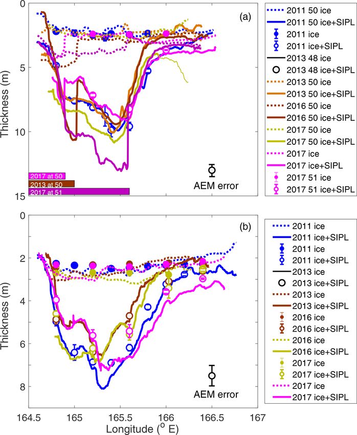
248                             C. Haas et al.: Airborne mapping of the sub-ice platelet layer under Antarctic landfast ice

   McMurdo Sound is characterized by intensive interaction         widely spaced sampling. Therefore observations of the kilo-
between the ice shelf, sea ice, and ocean (Gow et al., 1998;       metre scale and interannual variability of SIPL occurrence
Smith et al., 2001; Leonard et al., 2011; Robinson et al.,         and thickness are still rare or restricted to regions that are
2014; Langhorne et al., 2015). In particular, melting at the       accessible by on-ice vehicles (Hoppmann et al., 2015; Hun-
base of the Ross and McMurdo ice shelves results in the            keler et al., 2015a, b; Brett et al., 2020). Notably Hunkeler
seasonally variable presence of supercooled ice shelf water        et al. (2015a, b), Irvin (2018), and Brett et al. (2020) have
(ISW). A plume of supercooled ISW emerges from the Mc-             already demonstrated the capability of ground-based, single-
Murdo Ice Shelf and spreads north (Leonard et al., 2011;           frequency and multifrequency EM measurements to map the
Robinson et al., 2014), leading to the widespread formation        occurrence and thickness of the SIPL, using numerical inver-
and accumulation of frazil ice to form a sub-ice platelet layer    sion methods. The two latter studies have successfully repro-
under the fast ice (Fig. 1). This sub-ice platelet layer (SIPL)    duced the geometry of the SIPL known from earlier studies
is a poorly consolidated, highly porous layer of millimetre- to    (Barry, 1988; Dempsey et al., 2010; Langhorne et al., 2015).
decimetre-scale planar ice crystals (Hoppmann et al., 2020)        Using 4 years of ground-based EM data, Brett et al. (2020)
and is an important contributor to the sea ice mass balance        have studied the interannual SIPL variability and found that
in McMurdo Sound and along the coast of Antarctica in              the SIPL was thicker in 2011 and 2017 than in 2013 and
general (Smith et al., 2001; Gough et al., 2012; Langhorne         2016, in close relation to nearby polynya activity that con-
et al., 2015). Its presence and thickness are important indica-    tributes to variations in ocean circulation under the ice shelf.
tors of the occurrence of ISW near the ocean surface (Lewis        In spite of progress, details are lacking and the processes in-
and Perkin, 1985). Subsequently, the SIPL may consolidate          volved in the outflow of ISW from under the McMurdo Ice
and become incorporated into the solid sea ice cover to form       Shelf are still little known.
so-called incorporated platelet ice (Gow et al., 1998; Smith          In contrast to ground-based EM measurements where the
et al., 2001; Hoppmann et al., 2020). Due to the contributions     instrument height over the snow or ice surface is constant, in-
of platelet ice, sea ice thicknesses in Antarctic near-shore en-   strument height varies significantly with AEM measurements
vironments can be larger than in the pack ice zone further         due to unavoidable altitude variations of the survey aircraft.
offshore (Gough et al., 2012).                                     This makes the application of numerical inversion methods
   The SIPL in McMurdo Sound, its dependence on ocean              more complicated. Further, the development and calibration
processes, and its role in increasing sea ice freeboard and        of the empirical AEM SIPL retrieval algorithm requires that
thickness has been extensively studied for many years (e.g.        the electrical conductivity of the SIPL is known. The SIPL is
Gow et al., 1998; Mahoney et al., 2011; Robinson et al.,           an open matrix of loosely coupled crystals in approximately
2014; Price et al., 2014; Langhorne et al., 2015; Brett et al.,    random orientations, and its conductivity depends on its solid
2020). The spatial distribution of supercooled water and           fraction β (e.g. Gough et al., 2012; Langhorne et al., 2015),
platelet ice has been observed by means of local water             both of which are hard to measure directly. Observations and
conductivity, temperature, and depth (CTD) measurements            modelling over the past 4 decades suggest that β is quite low,
and drill-hole measurements on the fast ice (e.g. Lewis and        with a mean of β = 0.25 ± 0.09 (Langhorne et al., 2015) and
Perkin, 1985; Barry 1988; Dempsey et al., 2010; Leonard            range of 0.15–0.45 (e.g. Hoppmann et al., 2020).
et al., 2011; Mahoney et al., 2011; Robinson et al., 2014;            In this paper we develop a simple empirical algorithm for
Langhorne et al., 2015). These studies showed that a SIPL          the joint retrieval of SIPL and consolidated ice thicknesses
primarily occurs in a 20 to 30 km wide, 40 to 80 km long           from single-frequency AEM measurements that is supported
region extending from the northern tip of the McMurdo Ice          by an EM forward model and calibrated and validated by
Shelf in a northwesterly direction (Fig. 1) and locally near       coincident drill-hole measurements. We show that the SIPL
the coast of Ross Island. Drill-hole measurements showed           conductivity, and therefore its porosity or solid fraction, can
that at the end of the winter the thickness of the SIPL under      be obtained as a first step in the calibration of the method
first-year ice can be up to 7.5 m (Price et al., 2014; Hughes      with drill-hole data. We apply this algorithm to five surveys
et al., 2014), coinciding with more than 2.5 m of consoli-         carried out in November of 2009, 2011, 2013, 2016, and
dated sea ice. With multiyear ice, SIPL and consolidated ice       2017 by helicopter and fixed-wing aircraft. Using these tech-
thicknesses can be much larger, depending on location and          niques we demonstrate the ability of airborne electromag-
increasing with age.                                               netic induction (AEM) measurements to map the small-scale
   Electromagnetic induction sounding (EM) measurements            distribution of the SIPL under landfast sea ice with high spa-
are sensitive to the presence of layers of different electrical    tial resolution. We apply AEM to study the interannual vari-
conductivity in the subsurface. The presence and thickness         ability of the SIPL in McMurdo Sound from which we infer
of the porous, seawater-saturated SIPL can be retrieved be-        some previously unknown features of the ISW plume.
cause its electrical conductivity is in between that of the re-
sistive, consolidated sea ice above and the conductive seawa-
ter below. The technical and logistical difficulties of on-ice
and drill-hole measurements often only allow discontinuous,

The Cryosphere, 15, 247–264, 2021                                                       https://doi.org/10.5194/tc-15-247-2021
C. Haas et al.: Airborne mapping of the sub-ice platelet layer under Antarctic landfast ice                                        249

2     Methods and measurements                                          validated over drill-hole measurements and may be less ac-
                                                                        curate than reported above. Only in 2017 were we able to
2.1    AEM thickness surveys                                            use a Basler B67 airplane, permitting flights over the open
                                                                        water in the McMurdo Sound polynya which provided ideal
All measurements presented here were performed with a                   calibration conditions (Fig. 1f).
towed EM instrument (EM Bird) suspended below a heli-
copter or fixed-wing airplane and are thus named airborne               2.1.1   EM response to sea ice thickness and a sub-ice
EM (AEM) surveys. The EM Bird was flown with an average                         platelet layer
speed of 80 to 120 knots at mean heights of 16 m above the
ice surface (Haas et al., 2009, 2010). The instrument operated          Frequency-domain, electromagnetic induction (EM) sea ice
in vertical dipole mode with a signal frequency of 4060 Hz              thickness measurements rely on the active transmission of
and a spacing of 2.77 m between transmitting and receiving              a continuous, low-frequency “primary” EM field of one or
coils (Haas et al., 2009). The sampling frequency was 10 Hz,            multiple constant frequencies, penetrating through the resis-
corresponding to samples every 5 to 6 m depending on flying             tive snow and ice into the conductive seawater underneath.
speed. A Riegl LD90 laser altimeter was used to measure the             As the resistivity of cold sea ice and dry snow are approxi-
Bird’s height above the ice surface, with a range accuracy of           mately infinite (Kovacs and Morey, 1991; Haas et al., 1997),
±0.025 m. Positioning information was obtained with a No-               eddy currents are only induced in the seawater underneath.
vatel OEM2 differential GPS with a position accuracy of 3 m             These eddy currents generate a “secondary” EM field with
(Rack et al., 2013). Details of EM ice thickness sounding are           the same frequency as the primary EM field, but with a differ-
explained in the following sections.                                    ent amplitude and phase. The EM sensor measures the ampli-
   We have carried out five surveys over the fast ice in Mc-            tude and phase of the secondary field, relative to those of the
Murdo Sound, in November of 2009, 2011, 2013, 2016, and                 primary field, in units of parts per million (ppm) of the pri-
2017 (Fig. 1), i.e. in the end of winter when ice thickness             mary field. Amplitude and phase of the complex secondary
was near its maximum. The surveys covered several east–                 field are usually decomposed into real and imaginary signal
west-oriented profiles across the sound, as closely as possible         components, called in phase (I ) and quadrature (Q), respec-
from shore to shore, with approximate lengths of 50 km. Al-             tively.
though the exact number of profiles differed every year due
                                                                        I [ppm] = Amplitude [ppm] × cos (Phase [◦ ])
to weather restrictions, ice conditions, or technical issues, we
have attempted to cover the same profiles every year and                Q [ppm] = Amplitude [ppm] × sin (Phase [◦ ])
to collocate them with drill-hole measurements (Sect. 2.2).
The profiles repeated most often were located at latitudes of              With negligible sea ice and snow conductivities, measured
77◦ 400 , 77◦ 430 , 77◦ 460 , and 77◦ 500 S, i.e. 5.5 to 7.4 km apart   I and Q of the relative secondary field depend on the dis-
(Fig. 1).                                                               tance between the EM instrument and the ice–water inter-
   EM ice thickness measurements are affected by averag-                face and on the conductivity of the seawater. With known
ing within the footprint of the instrument, which results in            seawater conductivity, I and Q decay as an approximate neg-
the underestimation of maximum pressure ridge thicknesses               ative exponential with increasing distance (h0 + hi ) between
(e.g. Kovacs et al., 1995). However, the fast ice in McMurdo            the EM instrument and the ice–water interface, where h0 is
Sound is mostly undeformed and level. Over such level ice               instrument height above the ice and hi is ice thickness (see
without an underlying SIPL the agreement of EM thickness                Sect. 2.1.3 below; Haas, 2006; Pfaffling et al., 2007; Haas
estimates is within ±0.1 m of drill-hole measurements (Pfaf-            et al., 2009):
fling et al., 2007; Haas et al., 2009). McMurdo Sound there-
                                                                        I ≈ c0 × exp(−c1 × (h0 + hi )),                           (1a)
fore presents ideal conditions for EM ice thickness measure-
ments, and the levelness of the ice allows the application of           Q ≈ c2 × exp(−c3 × (h0 + hi )),                           (1b)
low-pass filtering to remove occasional noise from EMI in-
terference or episodic electronic drift that affects measure-           with constants c0...3 . Then, height above the ice–water inter-
ments over thick ice without losing significant information             face can be obtained independently from both I and Q from
on larger scales. Here, we have applied a running-window,               equations of the form
300-point median filter corresponding to a width of 1.5 to
                                                                        (h0 + hi ) ≈ −1/c1 × ln(I /c0 )                           (2a)
1.8 km to all data unless mentioned otherwise.
   However, the accuracy of 0.1 m stated above relies on                or
accurate calibration of the EM sensor, which is typically
achieved by flying over short sections of open water (Haas              (h0 + hi ) ≈ −1/c3 × ln(Q/c2 ).                           (2b)
et al., 2009). Unfortunately open water overflights were not
possible with the helicopter surveys between 2009 and 2013,                For ground-based measurements with an EM instrument
due to safety regulations. Then the calibration could only be           located on the snow or ice surface (i.e. h0 = 0 m), the

https://doi.org/10.5194/tc-15-247-2021                                                          The Cryosphere, 15, 247–264, 2021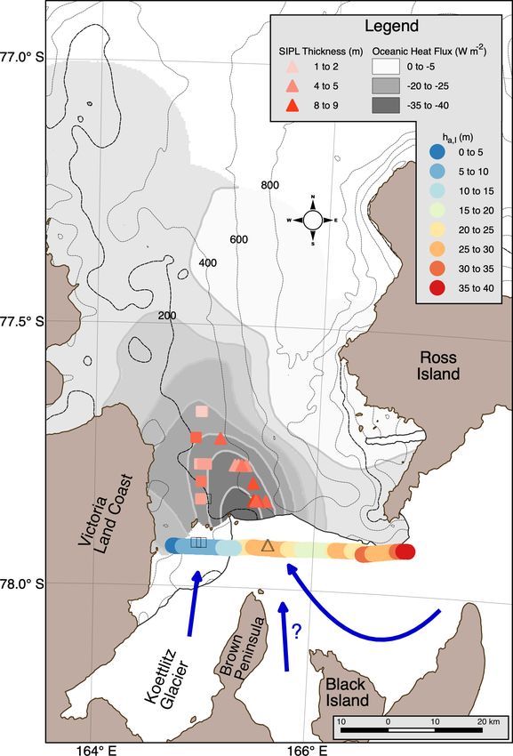
250                              C. Haas et al.: Airborne mapping of the sub-ice platelet layer under Antarctic landfast ice

distance to the ice–water interface corresponds to the to-         relation between I or Q and ice thickness described above
tal (snow-plus-ice) thickness hi (Kovacs and Morey, 1991;          (Eqs. 1, 3), smaller I and Q due to the presence of a SIPL
Haas et al., 1997). With airborne measurements, the variable       will result in apparent consolidated ice thickness estimates
height of the EM instrument above the snow or ice surface          ha that are larger than the true consolidated ice thickness hi .
h0 is measured with a laser altimeter. Then, total (ice-plus-      However, the derived consolidated ice thickness ha will be
snow) thickness is computed from the difference between the        less than the total ice plus SIPL thickness hi + hsipl because
electromagnetically derived height above the ice–water inter-      the thickness retrieval assumes negligible ice conductivity,
face and the laser-determined height above the snow or ice         which is an invalid assumption for the SIPL. Therefore the
surface:                                                           measured I and Q would be larger than they are for negligi-
                                                                   ble SIPL conductivity.
hi,I ≈ −1/c1 × ln(I /c0 ) − h0                             (3a)       As will be shown in Sect. 2.1.3, I and Q respond dif-
                                                                   ferently to the presence of a SIPL, and Q is in fact little
or                                                                 affected and can therefore still be used to retrieve hi . The
                                                                   presence of this layer can therefore be detected by devia-
hi,Q ≈ −1/c3 × ln(Q/c2 ) − h0                              (3b)
                                                                   tions between the apparent thicknesses derived from I and
(Pfaffling et al., 2007; Haas et al., 2009). Over typical saline   Q. The different responses of I and Q can also be used to
seawater, I (Eq. 1a) is 2 to 3 times larger than Q (Eq. 1b)        determine the thickness of the SIPL and thus to convert ap-
and has much better signal-to-noise characteristics (Haas,         parent thickness into consolidated ice and SIPL thicknesses
2006). It is therefore the preferred channel for ice thickness     (Sect. 2.1.4). In general, the thickness and conductivity of
retrievals in the Arctic and Antarctic (Haas et al., 2009). Be-    consolidated ice and the SIPL can be derived by means of
cause snow and ice are indistinguishable for EM measure-           full, least-square layered-earth inversion of airborne I , Q,
ments due to their low conductivity, no attempt is made here       and laser altimeter data and by potentially using more signal
to distinguish between them, and the terms ice thickness and       frequencies (e.g. Rossiter and Holladay, 1994; Pfaffling and
consolidated ice thickness are used throughout to describe         Reid, 2009; Hunkeler et al., 2015a, b). However, numerical
total, i.e. snow plus ice, thickness.                              inversion is computationally demanding and requires well-
                                                                   calibrated data with good signal-to-noise characteristics. In
2.1.2   Apparent thickness                                         addition, these algorithms require certain a priori knowledge
                                                                   about the stratigraphy of the ice, i.e. layers present and their
In the case of the presence of a SIPL, ice thickness retrievals    conductivities. The development and application of such al-
become significantly more difficult and will lead to large er-     gorithms is beyond the scope of this paper. Instead, here we
rors if the effect of the SIPL is not taken into account. Induc-   apply a simple empirical algorithm for the joint retrieval of
tion in the conductive SIPL results in an additional secondary     SIPL and consolidated ice thicknesses from single-frequency
field which mutually interacts with the secondary field in-        AEM measurements. The following section will outline the
duced in the water underneath. Thus the EM signal becomes          theoretical basis for this approach, including results from an
a function of both consolidated ice thickness and the thick-       EM forward model and a discussion of assumptions that need
ness and conductivity of the SIPL. The conductivity of the         to be made.
porous SIPL is higher than that of consolidated ice (∼ 0–
50 mS m−1 ; Haas et al., 1997) but most likely lower than that     2.1.3   Modelling EM responses over fast ice with a SIPL
of the seawater underneath (approximately 2700 mS m−1 in
McMurdo Sound; e.g. Mahoney et al., 2011; Robinson et al.,         To demonstrate the sensitivity of EM measurements to the
2014). Therefore, over consolidated ice underlain by a SIPL,       presence of a SIPL, and to evaluate the potential of determin-
the measured secondary field will be smaller than if there         ing its thickness, we performed extensive one-dimensional
were no SIPL and larger than if the SIPL were consolidated         forward modelling of the EM response to different SIPL
throughout and highly resistive.                                   thicknesses and conductivities. The I and Q components of
   Here we introduce the term “apparent thickness”, ha , to        the complex relative secondary field measured with horizon-
describe the ice thickness obtained from either I or Q follow-     tal coplanar coils over n horizontally stratified layers over-
ing the standard procedures and simple negative exponential        lying a homogeneous half-space can be calculated as (e.g.
relationship in Eq. (3) (Haas et al., 2009; Rack et al., 2013).    Mundry, 1984)
This is the thickness that one obtains if the presence of a SIPL                 Z∞
was not considered. The apparent thickness ha agrees with          (I + j Q) = r 2
                                                                                   λ2 R0 e−2λh0 J0 (λr) dλ.                    (4)
the true thickness hi if the ice has negligible conductivity.
                                                                                     0
Otherwise, in the presence of a conductive SIPL, the apparent
thickness ha will be more than the consolidated ice thickness,     This is a so-called Hankel transform utilizing a Bessel func-
but less than the total, consolidated ice plus SIPL thickness      tion of the first kind of order zero (J0 ), with r being the
hi + hsipl . Therefore, using the simple, negative-exponential     coil spacing, h0 the receiver and transmitter height above

The Cryosphere, 15, 247–264, 2021                                                        https://doi.org/10.5194/tc-15-247-2021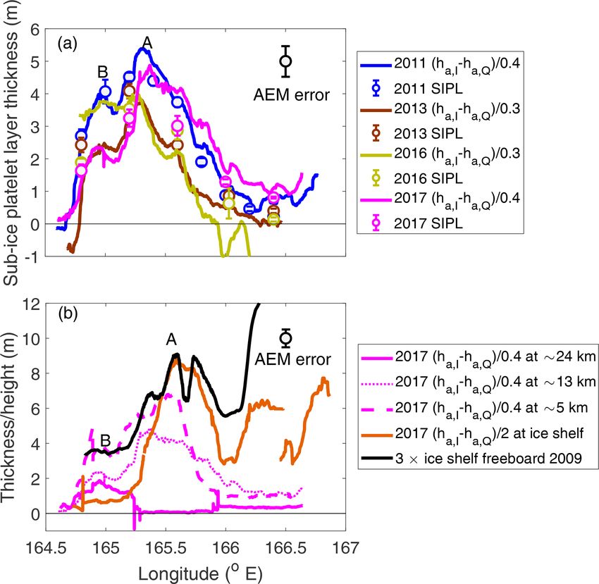
C. Haas et al.: Airborne mapping of the sub-ice platelet layer under Antarctic landfast ice 251
the ice, and λ the vertical integration constant. This equation SIPL is indistinguishable from consolidated ice, the result-
can only be solved numerically using digital filters. Here we ing curve is identical to measurements over consolidated ice
used the filter coefficients of Guptasarma and Singh (1997) only, i.e. generally following the form of Eq. (1).
that are, for example, implemented in a computer program In contrast, and not quite intuitively, initially Q changes
by Irvin (2019). R0 is called the transverse electric reflection little with increasing SIPL conductivity and thickness. In-
coefficient and is a recursive function of signal angular fre- deed, Q even increases slightly with increasing SIPL thick-
quency ω and the thickness and electromagnetic properties ness if the SIPL conductivity is high (e.g. larger than
of individual layers (electrical conductivity σ and magnetic 600 mS m−1 ). Only for very low SIPL conductivity (e.g. be-
permeability µ0 ): low 600 mS m−1 ) does Q decrease strongly, and for a con-
ductivity of 0 mS m−1 the curve is identical to the consoli-
Rn−1 = Kn−1 ,
dated ice case, as for I . Note that I is generally much larger
Rk−2 = (Kk−2 + Rk−1 uk−1 )/(1 + Kk−2 Rk−1 uk−1 ), than Q and that I is more strongly dependent on SIPL thick-
with ness. Therefore the sensitivity of I to the presence, thickness,
and conductivity of a SIPL is much larger than that of Q.
uk = exp(−2hk vk ), Figure 4 shows the apparent thicknesses, ha,I and ha,Q ,
vk = (λ2 + j ωµ0 σk )1/2 , that result from applying Eq. (3a, b) to the I and Q curves in
Fig. 3. Equation (3a, b) correspond to a SIPL conductivity of
Kk−1 = (vk−1 − vk )/(vk−1 + vk ).
0 mS m−1 that would be used if the presence of an SIPL were
In these equations n is the number of layers (four in this unknown or ignored. For example, and based on the same
paper: non-conductive air, sea ice and snow, SIPL, √ and sea- reasoning as above, Fig. 4 shows that the apparent thick-
water), k = 1 (air), . . . , 4 (seawater), and j = (−1). Fig- nesses agree with the total thickness hi + hsipl if the SIPL
ure 2 shows the general design of this four-layer case and conductivity was zero, i.e. indistinguishable from solid ice.
also the layer properties used for the computations which are If the conductivity of the SIPL was indistinguishable from
based on the typical conditions during our surveys in Mc- that of seawater (i.e. 2700 mS m−1 ), the obtained apparent
Murdo Sound. thicknesses are 2 m, i.e. the thickness of the consolidated ice
As the EM signal is ambiguous for variable layer thick- only. For the in-phase component, Fig. 4a shows that appar-
nesses and conductivities, we only calculate signal changes ent thicknesses for intermediate SIPL conductivities fall in
due to variable SIPL (layer 2) thicknesses hsipl and con- between, with increasing apparent thicknesses with decreas-
ductivities σsipl , keeping all other parameters constant and ing SIPL conductivities.
representative of our measurements: we chose instrument In contrast, apparent thicknesses derived from Q (Fig. 4b)
height h0 = 16 m, sea ice (layer 1) thickness hi = 2 m are similar to the consolidated ice thickness (2 m in this case)
and conductivity σi = 0 mS m−1 , and seawater (layer 3: in- for most SIPL conductivities. Only for SIPL conductivities
finitely deep, homogeneous half-space) conductivity σw = below 600 mS m−1 are there relatively stronger deviations,
2700 mS m−1 . SIPL conductivity σsipl was varied between 0 and for a SIPL conductivity of 0 mS m−1 the quadrature-
and 2700 mS m−1 in steps of 300 mS m−1 to study a range of derived apparent thickness equals the total thickness hi +
properties between the two extreme cases of negligible and hsipl . In summary these results show that the in-phase sig-
maximum seawater conductivity. SIPL thickness hsipl was nal I responds much more strongly to the presence of a SIPL
varied from 0 to 20 m to also include the most extreme poten- than the quadrature Q.
tial cases, such as to investigate the EM signal behaviour over Note that most in-phase curves level out for large SIPL
potentially thick platelet layers under multiyear ice or an ice thicknesses, the effect being exacerbated for higher SIPL
shelf. Note that we chose σi = 0 mS m−1 for simplicity, while conductivities (Fig. 3). This is due to the limited penetration
in reality consolidated sea ice still contains some brine that depth of EM fields in highly conductive media. Accordingly
can slightly raise its conductivity up to σi = 50 mS m−1 or the corresponding derived apparent conductivities level out
so (Haas et al., 1997). However, those small variations have with increasing SIPL thickness as well and are insensitive
little effect on the EM retrieval of consolidated ice thickness to further increases in SIPL thickness (Fig. 4a). In practice
(Haas et al., 1997; 2009). this means that the EM in-phase signals are only sensitive to
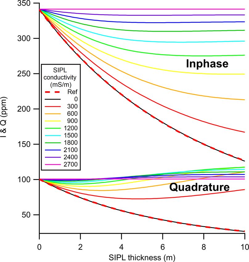
Figure 3 shows the dependence of I and Q model curves SIPL thickness changes up to a certain SIPL thickness and
over 2 m thick consolidated ice on variable SIPL thickness that the sensitivity decreases with increasing SIPL thickness
and conductivity obtained using the model of Eq. (4). As ex- and conductivity. In contrast, while Q is relatively insensitive
pected it can be seen that I and Q do not change with increas- to the presence and thickness of a SIPL for SIPL conduc-
ing SIPL thickness if the SIPL conductivity is 2700 mS m−1 , tivities above 600 mS m−1 , responses are non-monotonic for
i.e. if the SIPL is indistinguishable from seawater. I de- low SIPL conductivities and possess local minima at varying
creases exponentially with increasing SIPL thickness, the ef- SIPL thicknesses. As a result, apparent thicknesses derived
fect becoming more pronounced as SIPL conductivity de- from Q possess local maxima at variable SIPL thicknesses.
creases. When SIPL conductivity is 0 mS m−1 , i.e. when the
https://doi.org/10.5194/tc-15-247-2021 The Cryosphere, 15, 247–264, 2021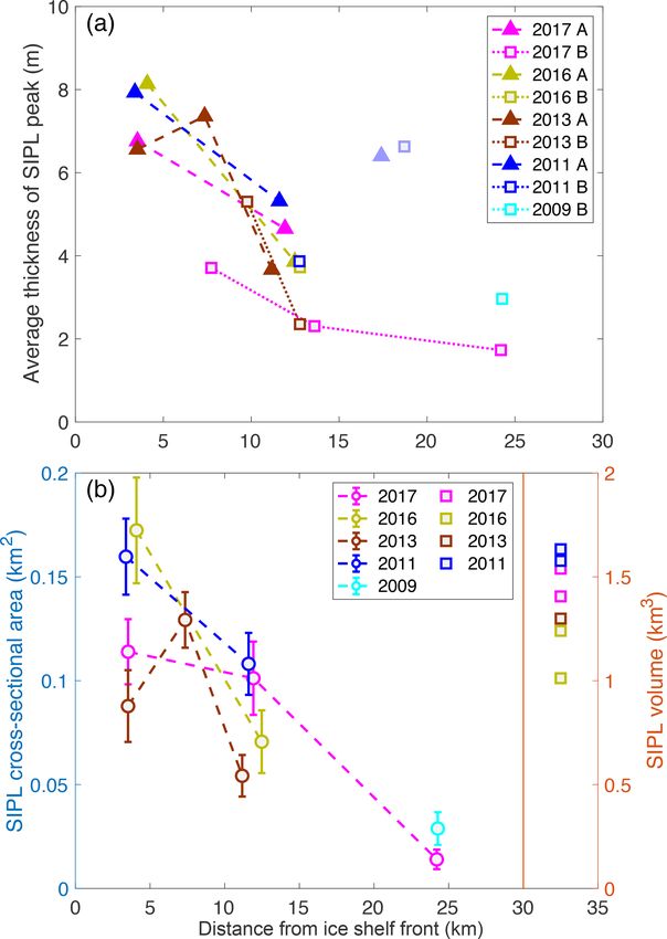
252                               C. Haas et al.: Airborne mapping of the sub-ice platelet layer under Antarctic landfast ice

Figure 1. Overview maps of the AEM surveys carried out in 2009, 2011, 2013, 2016, and 2017. (a) Regional overview and the location
of McMurdo Sound (green arrow) and boundaries of satellite images (red). (b–f) Locations of east–west profiles, overlaid on synthetic-
aperture radar (SAR) satellite images to show differences in general ice conditions and ice types (Brett et al., 2020; 2009/11: Envisat; 2013:
TerraSAR-X; 2016/17: Sentinel-1). Colours correspond to different apparent ice thicknesses ha,I (Sect. 2.1.2). Orange lines mark respective
fast ice edges. Bright areas to the south are the McMurdo Ice Shelf. Black dashed lines in (b, f) show tracks of ice shelf thickness surveys
used in Figs. 10a and 11 (Rack et al., 2013).

The Cryosphere, 15, 247–264, 2021                                                               https://doi.org/10.5194/tc-15-247-2021
C. Haas et al.: Airborne mapping of the sub-ice platelet layer under Antarctic landfast ice                                       253

                                                                      strument, and they will disagree if there is a SIPL under the
                                                                      consolidated ice. In general, the disagreement between ha,Q
                                                                      and ha,I will be larger the thicker the SIPL is. In other words,
                                                                      the presence and thickness of a SIPL can be retrieved from I
                                                                      and Q measurements, within limits.
                                                                         Using the behaviour described above, we derive the thick-
                                                                      ness of the consolidated ice hi directly from the apparent
                                                                      thickness of the Q measurement ha,Q , as it is mostly insen-
                                                                      sitive to the presence of a SIPL (Fig. 4b):
Figure 2. Schematic of the four-layer forward model to compute
EM responses over sea ice underlain by a SIPL with variable thick-    hi = ha,Q .                                                (5a)
ness and conductivity. T x and Rx illustrate transmitting and re-     Then, according to Fig. 4a the apparent thickness derived
ceiving coils, respectively. Instrument height h0 = 16 m, snow plus   from the in-phase measurements ha,I corresponds approxi-
ice thickness hi = 2 m, and water conductivity of 2700 mS m−1 are
                                                                      mately to the sum of consolidated ice thickness and a fraction
based on typical conditions during our surveys in McMurdo Sound.
                                                                      α of the true SIPL thickness:
                                                                      ha,I = hi + αhsipl ≈ ha,Q + αhsipl .                       (5b)
                                                                        Therefore we can derive hsipl from
                                                                      hsipl = (ha,I − hi )/α ≈ (ha,I − ha,Q )/α.                 (5c)
                                                                         The SIPL scaling factor α primarily depends on the SIPL
                                                                      conductivity and governs how much the true SIPL thickness
                                                                      is underestimated (Fig. 4a). The expected range of α values
                                                                      in Eq. (5c) and the uncertainty resulting from Eq. (5a) are
                                                                      shown in Fig. 5.
                                                                         Figure 5a shows the ratio of apparent thickness ha over
                                                                      “true” consolidated ice thickness hi which should be 1 ac-
                                                                      cording to Eq. (5a). However, it can be seen that the ratio
                                                                      strongly depends on hi and SIPL conductivity. In general the
                                                                      ratio is larger than 1 for a thin SIPL and smaller than 1 for
                                                                      a thick SIPL. The deviations from 1 decrease with increas-
                                                                      ing hi and with increasing SIPL conductivity. For example,
                                                                      for hi = 2 m and a SIPL conductivity of 1200 mS m−1 the
                                                                      ratio first increases to 1.27 and then decreases to a mini-
                                                                      mum of 0.7 before slowly increasing again (Fig. 5a). This
                                                                      means that with a true consolidated ice thickness of 2 m, typ-
                                                                      ical for end-of-winter first-year fast ice in McMurdo Sound,
                                                                      our method (Eq. 5a) overestimates or underestimates the true
Figure 3. In-phase I and quadrature Q responses to a 0 to 10 m
                                                                      consolidated ice thickness by up to 30 %. However, the actual
thick SIPL under 2 m thick consolidated ice for SIPL conductivi-
ties of 0 to 2700 mS m−1 computed with a three-layer EM forward       uncertainty depends on SIPL thickness and decreases with
model (see Fig. 2). Ref shows negative exponential curves for con-    increasing hi .
solidated ice with zero conductivity used for computation of I and       Figure 5b shows that α (Eq. 5c) decreases monotonically
Q apparent thicknesses using Eq. (2b).                                with increasing SIPL thickness and conductivity. For exam-
                                                                      ple, for a SIPL conductivity of 1200 mS m−1 it decreases
                                                                      from a value of 0.55 with no SIPL to values below 0.1 for
2.1.4   SIPL and consolidated ice thickness retrieval                 a very thick SIPL with hsipl  15 m. At a SIPL conductivity
        from measurements of I and Q                                  of 1200 mS m−1 it ranges between α = 0.4 and 0.3 for SIPL
                                                                      thicknesses between 3.7 and 6.2 m. There is little dependence
The contrasting behaviour of I and Q to variable SIPL thick-          on consolidated ice thickness hi . These results imply that the
ness and conductivity (Fig. 3) and the resulting contrasting          uncertainties due to unknown SIPL thickness (the parame-
behaviour of the derived apparent thicknesses (Fig. 4) can            ter that should actually be derived from this procedure) and
be used to retrieve SIPL and consolidated ice thicknesses.            SIPL conductivity can be quite large. This is because of the
The figures show that, if we derive apparent thicknesses from         increasingly limited sensitivity of the AEM measurements to
both the I and Q measurements independently, the results              increasing SIPL thicknesses discussed above with regard to
will agree if there is just consolidated ice under the EM in-         Fig. 4a and penetration depth.

https://doi.org/10.5194/tc-15-247-2021                                                        The Cryosphere, 15, 247–264, 2021
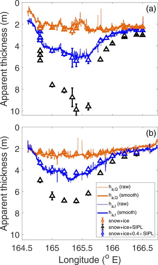
254                             C. Haas et al.: Airborne mapping of the sub-ice platelet layer under Antarctic landfast ice

2.2    Drill-hole validation measurements

At 55 sites over all 5 years of observation, drill-hole mea-
surements were performed under the flight tracks of the EM
Bird to measure the thickness of snow, sea ice, and the SIPL,
and the freeboard of the ice. The protocol at each drill site has
been described in Price et al. (2014) and Hughes et al. (2014).
At each site, five measurements were made at the centre and
corners of a 30 m wide “cross”. Sea ice thickness and the
depth of the bottom of the sub-ice platelet layer were mea-
sured with a classical T-bar at the end of a tape measure low-
ered through the ice and pulled up until resistance was felt
(Haas and Druckenmiller, 2009; Gough et al., 2012). This
is an established method in the absence of a sub-ice platelet
layer, with ice thickness accuracies of 2 to 5 cm. However,
the bottom of the unconsolidated sub-ice platelet layer is of-
ten fragile and may be gradual, such that pull resistance may
only increase gradually and may be difficult to feel (Gough
et al., 2012). This is further complicated by the frequent
presence of ice platelets inside the drill hole causing addi-
tional resistance and impeding detection of the water level
within the hole. Ice crystals may be jammed between the T-
anchor and the bottom of the consolidated ice, hampering
the accurate determination of sea ice thickness. Following
Price et al. (2014), we assume typical relative errors (1 stan-
dard deviation) for the drill-hole sea ice and sub-ice platelet
layer thicknesses to be ±2 % and ±5 % to 30 %, respectively.
Snow thickness was measured on the cross lines at 0.5 m in-
tervals using a ruler (2009, 2011, and 2013) or a Magnaprobe
(2016 and 2017; Sturm and Holmgren, 2018). Throughout
this paper we have added snow and ice thickness to comprise
total consolidated ice thickness hi .

3     Results

3.1    Apparent ice thicknesses in McMurdo Sound

The SAR images in Fig. 1b–f show that the fast ice in Mc-
Murdo Sound can be quite variable, with regard to both the
location of the ice edge and the types of first-year ice that are   Figure 4. Apparent thicknesses resulting from applying simple
present (Brett et al., 2020). Due to break-up events during         negative-exponential equations like in Eq. (3a, b) to the I and Q
the winter there can be refrozen leads with younger and thin-       curves in Fig. 3.
ner ice, or larger areas of thinner ice, as can for example be
seen in 2013 in the northeast of the panel. These variable ice
conditions result in variable thickness profiles that are indis-    2.5 m, in the eastern side of the sound, in good agreement
tinguishable from small undulations due to instrument drift.        with other studies (Price et al., 2014, Brett et al., 2020) and
The SAR images also show the presence of multiyear land-            with our drill-hole measurements (see below). On the west-
fast ice in some years, in particular in 2009. The multiyear        ern side of the sound much thicker ice, up to 6 m in apparent
ice is much thicker than the first-year ice, and we have few        thickness, can be seen. The regional distribution and thick-
drill-hole measurements there. Therefore, results over multi-       ness of this thick ice coincides with our general knowledge
year ice are not included here.                                     of the distribution of the ISW plume and the SIPL in the re-
   Figures 1b–f also show the apparent thickness ha,I de-           gion (Dempsey et al., 2010; Langhorne et al., 2015). In par-
termined from the in-phase component along the profiles.            ticular, the data show that apparent ice thicknesses are much
In general it can be seen that ha,I ranges between 2.0 and          larger near the ice shelf than farther north, in agreement with

The Cryosphere, 15, 247–264, 2021                                                        https://doi.org/10.5194/tc-15-247-2021
C. Haas et al.: Airborne mapping of the sub-ice platelet layer under Antarctic landfast ice                                             255

Figure 5. Ratio of ha,Q /hi (a; see Eq. 5a) and α = (ha,I −hi )/hsipl
(b; see Eq. 5c) vs. SIPL thickness, at different consolidated ice
thicknesses hi between 2 and 6 m and different SIPL conductivi-
ties between 300 and 2400 mS m−1 . Curves follow from curves in         Figure 6. Apparent AEM thicknesses ha,Q (orange lines) and ha,I
Figs. 3 and 4. Black boxes show the range of ha,Q /hi and α values      (blue lines) along E–W profiles at (a) 77◦ 500 S and (b) 77◦ 460 S
resulting from the calibration (Sect. 3.2).                             in November 2011, approximately 3 and 11 km from front of Mc-
                                                                        Murdo Ice Shelf, respectively. Dotted lines are raw data, while solid
                                                                        lines are filtered with a 300-point median filter. Triangles show
                                                                        mean and standard deviation of drill-hole measurements at cali-
the fact that the ISW plume emerges from the ice shelf and              bration points. Consolidated ice (snow plus ice; orange), consol-
then spreads north. However, the obtained apparent thick-               idated ice plus SIPL thickness (black), and consolidated ice plus
nesses are much smaller than what is known from drill-hole              (α = 0.4) × SIPL thickness (blue; Eq. 5c).
measurements, when SIPL thickness is taken into account.
These results confirm the results of our modelling study and
demonstrate that the in-phase measurements are sensitive to
the presence and thickness of a SIPL.                                   Fig. 9 we plotted thickness downwards to illustrate more in-
   In general, apparent thicknesses ha,Q derived from the               tuitively the bottom of the consolidated ice and SIPL. It can
quadrature measurements show much less variability. We                  be seen that ha,Q and ha,I agree with each other quite well in
will present them below where we show the derived consoli-              the east (right) and show an ice thickness of approximately
dated ice thicknesses (Sect. 3.2, Fig. 6).                              2.0 to 2.5 m, in agreement with the consolidated ice thick-
                                                                        ness in that region. However, farther west (left), in the re-
3.2   Calibration of consolidated ice and SIPL thickness                gion of the ISW plume and thicker SIPL, the curves deviate
                                                                        from each other. While ha,Q changes relatively little, ha,I in-
The behaviour of ha,Q and ha,I can be seen much better                  creases strongly. The curves join again in the farthest west,
when vertical cross sections of individual profiles are plot-           where the ISW plume is known to vanish (Robinson et al.,
ted. This is shown in Fig. 6 for one profile near the ice shelf         2014). While both curves follow the expected behaviour re-
edge (Fig. 6a) and one farther north (Fig. 6b). The figure also         sulting from the model results well (Sect. 2.1.3), and while
shows drill-hole data for comparison. Note that here and in             ha,Q is in reasonable agreement with the drill-hole measure-

https://doi.org/10.5194/tc-15-247-2021                                                            The Cryosphere, 15, 247–264, 2021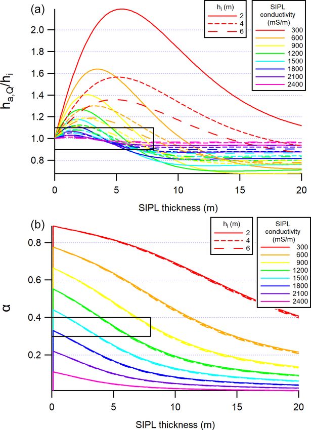
256 C. Haas et al.: Airborne mapping of the sub-ice platelet layer under Antarctic landfast ice
Table 1. Summary of drill-hole calibration results showing the number of drill-hole measurements N, derived scaling factor α (Eq. 5c), SIPL
conductivity σSIPL , and solid fraction β. Data from several years with similar behaviour were pooled to increase the number of data points
for more reliable fits.
Year (November) N α (95 % conf. int.) σSIPL (mS m−1 ) β
2009, 2011 and 2017 46 0.40 ± 0.07 900–1500 0.16–0.47
2013 and 2016 9 0.30 ± 0.15 1000–1800 0.09–0.43
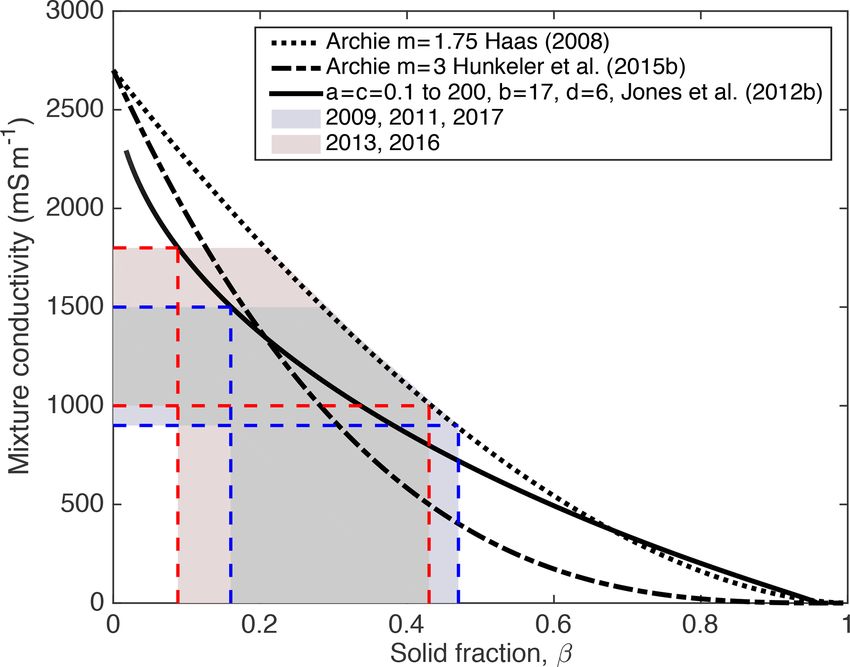
Figure 8. Conductivity vs. solid fraction for porous media accord-
ing to theories by Archie (1942) with different cementation factors
m = 1.75 and 3 and Jones et al. (2012b; black curves). Coloured
areas show the range of SIPL conductivities derived from compar-
ison of drill-hole and EM SIPL thicknesses (Fig. 5b, Table 1) and
Figure 7. Scatter plot of EM derived vs. drill-hole consolidated ice
resulting solid fractions according to the different theories.
thickness (hi ; filled symbols) and total thickness (hi + hsipl ; open
symbols), with symbol colour denoting year of measurement. To-
tal thickness (hi + hsilp ) was calculated with α = 0.4 (best fit value
0.40±0.07, N = 46) for 2009, 2011, and 2017 and α = 0.3 for 2013
and 2016 (best fit value 0.30 ± 0.15, N = 9); see Table 1. Error bars
show ice thickness variability at each calibration location (five drill sites. These values for α are summarized in Table 1. For first-
holes) or within the approximate EM footprint (the latter are too year, land-fast sea ice in 2009, 2011, and 2017, there are N =
small to be visible at the scale of the graph). The black line is 1 : 1. 46 coincident measurements and they yield a best fit value of
N = 9 for 2009, N = 26 for 2011, N = 5 for 2013, N = 4 for 2016, α = 0.40 ± 0.07. A SIPL factor of α = 0.4 has been used for
and N = 11 for 2017; thus total N = 55. those years henceforth. Fewer drill-hole measurements were
available in 2013 and 2016 (N = 9 in total), resulting in a
best fit of α = 0.30 ± 0.15. We therefore use an SIPL scaling
ments of consolidated ice thickness hi , ha,I strongly underes- factor of α = 0.3 for 2013 and 2016 from here on.
timates total ice thickness hi + hsipl . Therefore, according to With these α values we can then convert all in-phase
Eq. (5b), the drill-hole measurements of SIPL thickness can and quadrature measurements into total consolidated ice plus
be multiplied by a factor of α = 0.4 for best agreement with SIPL thickness. Figure 7 shows a scatter plot of thicknesses
the in-phase AEM measurements. Note that this behaviour thus derived vs. total drill-hole thicknesses. It demonstrates
and value for α are also in good agreement with the model that EM-derived and drill-hole thicknesses agree very well,
results and with the range of α values predicted by Fig. 5b. with a best fit line of slope 1.00±0.05 and intercept 0.0±0.2
The good agreement between ha,Q and hi from the drill- (95 % confidence intervals) and root-mean-square error of
hole data strongly supports our approach of using ha,Q as the 0.47 m. Based on this and the discussion of Fig. 5 above we
best estimate for hi (Eq. 5a). This approach will be evaluated also estimate that the systematic error associated with the un-
below (Fig. 7). In order to determine the best values for α, certainty in the simplified processing of the ha,Q and ha,I
we have fit the drill-hole-measured ice and SIPL thicknesses data and the choice of α yields a data reduction model uncer-
against (ha,I − ha,Q ) measured by the EM Bird at the same tainty of ±0.5 m.
The Cryosphere, 15, 247–264, 2021 https://doi.org/10.5194/tc-15-247-2021C. Haas et al.: Airborne mapping of the sub-ice platelet layer under Antarctic landfast ice 257
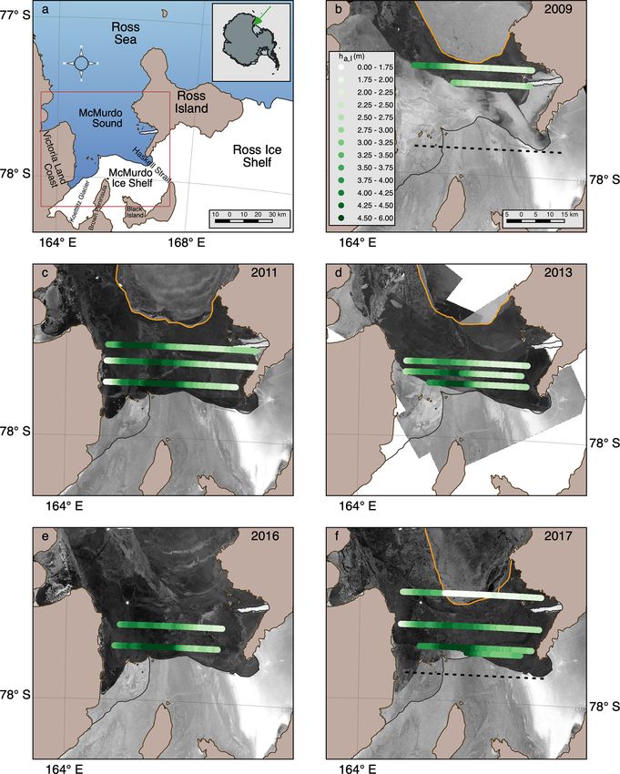
Figure 9. Interannual variability of AEM-derived and drill-hole-consolidated ice hi (stippled lines and filled symbols) and total thickness
hi + hsipl (solid lines and open symbols) along E–W transects at similar latitude (median filtered). (a) Transects at approximately 77◦ 480 to
77◦ 510 S in November 2011, 2013, 2016, and 2017, approximately 3 to 5 km from the McMurdo Ice Shelf front. Horizontal bars indicate
very thick MY ice present in the west along part of the profiles in 2013 and 2017. (b) Transect at approximately 77◦ 460 S in November 2011,
2013, 2016, and 2017, approximately 11 km from McMurdo Ice Shelf front. Note different y axis scales, i.e. thicker SIPL farther south. The
data reduction model uncertainty in AEM total thicknesses (snow + ice + SIPL) is shown.
3.3 SIPL conductivity and solid fraction Archie’s law being the best known (Archie, 1942). Figure 8
shows the horizontal conductivity for Archie’s law with tor-
The SIPL scaling factors, α, are highly sensitive to SIPL tuosity factor and saturation exponent set to 1 (e.g. Kovacs
conductivity and thickness (Fig. 5b). However, with known and Morey, 1986) and cementation factor m = 1.75 (Haas
α and SIPL thicknesses from the drill-hole calibrations in et al., 1997) and m = 3 (Hunkeler et al., 2015b), as the solid
Sect. 3.2 (Table 1), we can narrow down the range of possible fraction is increased from 0 to 1. For sea ice specifically,
SIPL conductivities, in particular as the range of SIPL thick- Jones et al. (2012a) have used a simple conductivity model
nesses only extends between 0 and 8 m. The corresponding (Jones et al., 2012b) to derive parameters for an ice/brine
region of α values and SIPL thicknesses has been marked “unit cell”. Each unit cell consists of a single, isolated, cubi-
in Fig. 5b. It can be seen that most curves within this re- cal brine pocket with sides of relative dimension d (unitless)
gion have conductivities between 900 and 1800 mS m−1 . The and three connected channels in perpendicular directions
range of conductivities resulting from different α in the dif- (two horizontal and one vertical direction), each with relative
ferent years is listed in Table 1. dimensions c×a×b (also unitless). Jones et al. (2012b) found
In order to relate the conductivities to a solid fraction that the relative dimensions that fit the observed in situ DC
within the SIPL, we need a model of electrical conductivity,
https://doi.org/10.5194/tc-15-247-2021 The Cryosphere, 15, 247–264, 2021258 C. Haas et al.: Airborne mapping of the sub-ice platelet layer under Antarctic landfast ice
horizontal and vertical resistivities depend not only on sea ice 3.5 Evidence of persistent, recurring SIPL pattern
temperature but also on structure. In particular, for Antarctic
incorporated platelet ice at −5 ◦ C, the shape of the inclusions
has relative brine pocket dimensions a ≈ 1, b ≈ 17, c ≈ 0.6, Close inspection of the thickness data in all years and at all
and d ≈ 6 (see Jones et al., 2012a, for details). In addition, latitudes reveals the presence of persistent, recurring local
Jones et al. (2012b) have shown for Arctic first-year sea ice maxima or clear shoulders in the thickness profiles. Typical
that there is a dramatic change in these parameters with tem- examples that were identified are illustrated by A and B in the
perature, with a, c, and d becoming relatively larger, while repeated profiles along transect 77◦ 460 S in 2011, 2013, 2016,
b drops. This behaviour would also be expected in incorpo- and 2017 in Fig. 10a. Figure 10b shows that these maxima are
rated platelet ice. We shall therefore assume that the shape of also present in a series of profiles at increasing latitude or de-
the inclusions in the SIPL is similar to that of incorporated creasing distance from the front of the McMurdo Ice Shelf.
platelet ice (as observed by Jones et al., 2012a) but that brine While Fig. 10a also shows the typical interannual variabil-
inclusion and void dimensions are very much larger because ity of up to 2 m in SIPL thickness already seen in Fig. 9,
they are very close to the freezing point. Consequently, we Fig. 10b nicely demonstrates the decreasing SIPL thickness
calculate the relationship between solid fraction and conduc- with increasing distance from the ice shelf already indicated
tivity from Jones et al. (2012b), by varying a and c, while by the differences between Fig. 9a and b.
keeping b and d constant and hence changing the solid and For comparison, Fig. 10b also includes data from AEM
liquid content of the SIPL (see Fig. 8). and laser altimeter surveys of the McMurdo Ice Shelf near
From these curves, and the conductivities derived from the its front at 77◦ 550 S (see ice shelf locations in Fig. 11) in
comparison of EM and drill-hole SIPL thicknesses (Fig. 5b, November 2009 and 2017. It shows the ice freeboard in
Table 1), we can estimate the corresponding solid fraction 2009 from Rack et al. (2013) and an uncalibrated measure
of the SIPL, with data in Fig. 8 grouped into two sets for of the SIPL thickness beneath the ice shelf. The latter was
the range of conductivities for α = 0.4 in blue (2009, 2011, derived from the difference between in-phase and quadrature
2017) and α = 0.3 in red (2013, 2016). Thus the airborne apparent thicknesses, ha,I −ha,Q , but no scaling was applied.
measurements imply that the range of solid fractions in Note that the ratio between ha,Q and hi and scaling factor α
the SIPL lies between 0.1 and 0.5, but values are lower in (Eqs. 5) under the 20 to more than 50 m thick ice shelf could
2013 and 2016 than in 2009, 2011, and 2017 (see Table 1 be quite different than under 2 m thick sea ice and that no
and Fig. 8). We shall discuss this interannual variability in calibration measurements were available.
Sect. 3.4.1. Figure 10b shows that the locations of the local maxima
in SIPL thickness under the ice shelf in 2017 coincide very
3.4 Spatial and interannual variability of the SIPL well with the ice shelf freeboard of Rack et al. (2013) in
2009. This could be due to preferential accretion of marine
3.4.1 Interannual variability and latitudinal differences ice in those locations or due to the increased buoyancy from
the SIPL under the ice shelf (Rack et al., 2013). Even more
Figure 9 shows the distribution of consolidated ice thickness
importantly, the locations of the SIPL thickness maxima un-
hi and total ice thickness hi + hsipl along two E–W transects
der the ice shelf coincide approximately with the locations of
in 2011, 2013, 2016, and 2017, derived from the AEM sur-
SIPL thickness maxima under the fast ice to the north, pro-
veys and drill-hole data. The transects are 3 to 5 km (Fig. 9a)
viding evidence that the structure of the SIPL under the fast
and 11 km north of the ice shelf front Fig. (9b). In 2013
ice is directly linked to the geometry of the ISW outflow from
and 2017 there was some multiyear ice in southwestern Mc-
under the ice shelf.
Murdo Sound (see Fig. 1d and f), and at these locations both
The local maxima A and B illustrated in Fig. 10 can be vi-
consolidated ice and the SIPL show abrupt increases in thick-
sually identified in some transects from all years 2009, 2011,
ness.
2013, 2016, and 2017 and their positions are shown in re-
The figure shows a generally thicker SIPL along the south-
gional context on the map in Fig. 11. The peaks clearly orig-
ern transect, in agreement with the notion of a thick SIPL that
inate under the ice shelf and propagate beneath the sea ice,
emerges from under the ice shelf and thins towards the north,
carried northward by the ISW plume. The thickest peak A ap-
with increasing distance from the ice shelf. Over the first-
pears to be carried westward, as is also visible in Fig. 10. The
year ice, on both transects hi varies by less than 0.75 m from
westward displacement of this peak may be supported by the
year to year, while variations of up to 2 m are seen in SIPL
Coriolis force acting on the northward-flowing ISW (Robin-
thickness hsipl . While there is interannual variability in the
son et al., 2014), as suggested by the modelling of Cheng
thickness of the SIPL, the shape of the thickness distribution
et al. (2019) and Holland and Feltham (2005). Peak B is far-
is remarkably consistent from year to year.
ther west and appears to originate from under the ice shelf
near the Koettlitz glacier. Its course is more northerly as it
may be constrained by the 200 m isobath. While the ice shelf
thickness measurements near the front are uncalibrated, they
The Cryosphere, 15, 247–264, 2021 https://doi.org/10.5194/tc-15-247-2021C. Haas et al.: Airborne mapping of the sub-ice platelet layer under Antarctic landfast ice 259 Figure 10. (a) SIPL thickness along 77◦ 460 S in 2011, 2013, 2016, and 2017, approximately 11 km from McMurdo Ice Shelf front. Recurring local maxima or shoulders in thickness are identified at A and B. (b) SIPL thickness profiles in November 2017 at different distances from McMurdo Ice Shelf front (pink lines), at approximately 24 km (solid), 13 km (dotted), and 5 km (dashed). The figure also shows uncalibrated, scaled SIPL thickness beneath the ice shelf in 2017 (brown) and scaled ice shelf freeboard in 2009 (black; from Rack et al., 2013), at 77◦ 550 S. The ice shelf data are smoothed by a moving-average filter of window size 50. Local thickness maxima are identified at A and B. The data reduction model uncertainty in AEM total thicknesses (snow + ice + SIPL) is shown. are generally in agreement with thicknesses from 1960–1984 gral was calculated for cross sections with SIPL thicknesses (McCrae, 1984) and from 2015 (Campbell et al., 2017). of at least 1 m. A few thickness surveys had to be ended be- Finally, Fig. 12a shows the thickness of peaks A and B fore SIPL thickness decreased below 1 m in the west, near the from Fig. 11 vs. latitude. Thicknesses were averaged over a coast. In these cases data were simply extrapolated following width 0.1◦ of longitude centred on the peak location to be the generally steeply decreasing thickness gradients found in statistically more representative. Although quite noisy, the the west (e.g. Fig. 10a). These integral thicknesses are less figure shows that peak A is generally larger than peak B, influenced by the peak thicknesses but more representative and that both are decreasing with distance from the ice shelf of the overall volume of SIPL at the different distances from front. Peak A decreases from a maximum SIPL thickness the ice shelf. However, the same general behaviour as with of 8 m approximately 3 km from the front to less than 3 m peak thicknesses in Fig. 12a can be seen, with all peaks de- at 24 km, i.e. over a distance of 21 km. The relatively large creasing in thickness with distance from the ice shelf, from scatter of up to 2 m at single locations is due to the described south to north. The figure also confirms that SIPL thicknesses interannual variability and retrieval uncertainty. At the north- and therefore volumes were larger in 2011 and 2017 than in ernmost transect 24 km from the ice shelf (77◦ 400 S) only one 2013 and 2016. These results are in general agreement with peak was identifiable. It is quite possible that the converging SIPL volumes derived from ground-based EM surveys by paths of peaks A and B have merged at that latitude. Brett et al. (2020) also shown in Fig. 12b. Note that absolute In contrast, Fig. 12b shows integrated SIPL thicknesses values are difficult to compare because Brett et al. (2020) de- across the complete individual east–west transects. The inte- https://doi.org/10.5194/tc-15-247-2021 The Cryosphere, 15, 247–264, 2021
260                               C. Haas et al.: Airborne mapping of the sub-ice platelet layer under Antarctic landfast ice

                                                                       Figure 12. (a) SIPL thickness of peaks A and B (averaged over 0.1◦
                                                                       of longitude) vs. distance from ice shelf front for all years 2009,
Figure 11. Bathymetric map of McMurdo Sound showing the loca-
                                                                       2011, 2013, 2016, and 2017 (see Fig. 11). (b) East–west cross-
tion of local maxima in SIPL thickness, with peak A as triangles and
                                                                       sectional area through the SIPL region (defined as greater than 1 m
B as squares for all years 2009, 2011, 2013, 2016, and 2017. The
                                                                       thickness). Simultaneous SIPL volumes over a 675 km2 area in the
magnitudes of the local maxima are coloured proportionally to the
                                                                       central McMurdo Sound from Brett et al. (2020) are shown on the
thickness of the peak, with darker orange for thicker average SIPL.
                                                                       right (squares). Error bars assume a ±0.5 m data reduction model
Open symbols denote peaks whose absolute thicknesses were un-
                                                                       uncertainty in EM SIPL measurements (Sect. 3.2).
certain. Coloured horizontal line shows ice shelf ha,I profile flown
in 2017 with locations of corresponding A and B peaks identified.
Contours in grey are proportional to negative ocean heat flux from
Langhorne et al. (2015). Blue arrows indicate possible paths of sur-   of 0.47 m. This uncertainty is partially due to the EM mea-
face ISW (based on Robinson et al., 2014).                             surement noise on the order of 10 ppm in I and Q, whose
                                                                       effect on retrieved ice thicknesses increases with increasing
                                                                       thickness and decreasing I and Q signals, due to the negative
rived their average results from data that were spatially grid-        exponential EM response to increasing ice thickness.
ded across the central McMurdo Sound.                                     In a few instances, we also observed that the retrieved
                                                                       SIPL thicknesses were actually negative but still within the
                                                                       derived rms errors (e.g. Fig. 10a). Negative values arise when
4   Discussion                                                         the in-phase-derived apparent total thickness is smaller than
                                                                       the quadrature-derived apparent consolidated ice thickness
In this study we have presented a new, simple method to                (Eq. 5c), which can happen when the SIPL is very thin or
map the distribution and thickness of a sub-ice platelet layer         absent. The quadrature signals are not only much weaker
(SIPL) by means of airborne EM surveying. The accuracy of              than the in-phase signals (Fig. 3), but they are also subject
the method was assessed with theoretical considerations and            to stronger electronic instrument drift. This makes the detec-
by means of comparisons with drill-hole data. Regression of            tion of SIPL layers thinner than 0.5 m very challenging.
EM results with drill-hole data showed very low bias with a               In addition to uncertainties due to instrument effects, vari-
slope of 1 and intercept of 0 m, but a root mean square error          able SIPL conductivities contribute to variations in the EM

The Cryosphere, 15, 247–264, 2021                                                            https://doi.org/10.5194/tc-15-247-2021
You can also read