Wall Street and the Housing Bubble - Ing-Haw Cheng , Sahil Raina , and Wei Xiong September 2012
←
→
Page content transcription
If your browser does not render page correctly, please read the page content below
Wall Street and the Housing Bubble

                       Ing-Haw Cheng†, Sahil Raina‡, and Wei Xiong§

                                            September 2012

                                                 Abstract

               We analyze whether mid-level managers in securitized finance were aware
               of the housing bubble in 2004-2006 using their personal home transaction
               data. We find little evidence of them timing the bubble or exercising
               cautious behavior in purchasing homes on average, relative to two
               uninformed control groups: one composed of non-real estate lawyers and the
               other of non-housing equity analysts. Our findings cast doubt on the
               popular “inside job” view of the recent financial crisis that Wall Street
               employees knowingly ignored warning signs of the housing bubble.

               JEL Codes: G01, G20, G21, G23, G24

               Appendices available online

    †
       Ross School of Business, University of Michigan, Ann Arbor, MI 48109-1234, e-mail: ingcheng@umich.edu,
http://webuser.bus.umich.edu/ingcheng.
     ‡
       Ross School of Business, University of Michigan, Ann Arbor, MI 48109-1234,
http://webuser.bus.umich.edu/sraina.
     §
       Department of Economics and Bendheim Center for Finance, Princeton University, Princeton, NJ 08540, e-
mail: wxiong@princeton.edu, http://www.princeton.edu/~wxiong.
    The authors thank Vu Chau, Kevin Chen, Andrew Cheong, Tiffany Cheung, Alex Chi, Andrea Chu, Wenjing
Cui, Christine Feng, Kelly Funderburk, Elisa Garcia, Holly Gwizdz, Jisoo Han, Bret Herzig, Ben Huang, Julu
Katticaran, Olivia Kim, Eileen Lee, Yao Lu, Shinan Ma, Amy Sun, Stephen Wang, and Daniel Zhao for excellent
research assistance. The authors are also grateful to Nick Barberis, Roland Benabou, Harrison Hong, Atif Mian,
Amit Seru, and seminar participants at the Federal Reserve Bank of Philadelphia, NBER Behavioral Finance
Meeting, NBER Summer Institute, and University of Michigan for helpful discussion and comments.
Following financial crises, concerns often arise about insiders having taken advantage of
outsiders by first pumping up asset prices and then selling before prices crash. In the aftermath
of the collapse of the Internet bubble in early 2000s, charges of conflicts of interest among sell-
side analysts within investment firms resulted in lawsuits and settlements in the billions of
dollars. After the collapse of Enron and WorldCom, outrage regarding executives and directors
enriching themselves by selling their shares shortly before their companies’ failures led to the
Sarbanes-Oxley Act of 2002. These concerns have resurfaced after the recent crisis on Wall
Street. A popular view posits that moral hazard caused Wall Street employees to ignore clear
warning signs about the presence of an unprecedented housing bubble and the imminent risk of
the bubble bursting. According to the Financial Crisis Inquiry Report (2011) of the Financial
Crisis Inquiry Commission formed by the U.S. Congress:
“In the decade preceding the collapse, there were many signs that house prices
were inflated, that lending practices had spun out of control, that too many
homeowners were taking on mortgages and debt they could ill afford, and that
risks to the financial system were growing unchecked. Alarm bells were clanging
inside financial institutions, regulatory offices, consumer service organizations,
state law enforcement agencies, and corporations throughout America, as well as
in neighborhoods across the country. Many knowledgeable executives saw trouble
and managed to avoid the train wreck.”
The Academy Award-winning documentary “Inside Job” vividly attributes the crisis to Wall
Street insiders taking advantage of uninformed borrowers and investors and blames employees in
securitized finance for selling securities backed by dubious-quality subprime mortgage loans to
uninformed investors. Building on the premise that Wall Street employees anticipated the
housing bubble earlier than others, this inside job view holds that the crisis was avoidable if
appropriately designed incentives and necessary government oversight were in place.
However, there are open disagreements among policy makers and academic researchers
about this view, and, in particular, whether Wall Street employees were truly aware of the
housing bubble. Interestingly, one of the two minority reports contained in the Financial Crisis
Inquiry Report (2011) challenges the premise that warning signs were clear to people in finance,
and instead attributes them to hindsight:
“There always are [warning signs] if one searches for them; they are most visible
in hindsight, in which the Commission majority, and many of the opinions it cites
for this proposition, happily engaged.”
1Motivated by this disagreement and the importance of this issue, we examine the following
question: What did Wall Street employees know about the housing bubble and when did they
know about it? The challenge in addressing this question lies with how to isolate their beliefs
about the housing market from their job incentives.
This paper confronts this challenge by exploiting the special nature of personal transactions
in housing markets. Different from typical financial assets, residential homes are an
indispensable part of everyone’s life. A home typically exposes its owner to house price risk in
the hundreds of thousands of dollars. As a result, even employees in the financial industry,
despite their relatively high incomes, should have maximum incentives to make informed home-
transaction decisions regardless of any potentially biased incentive from their jobs. Building on
this insight, we use their personal home transactions during the housing bubble to extract
information about their beliefs regarding the housing markets at the time.
We focus on a sample of mid-level managers who worked directly in the securitization
business, a central part of the housing bubble. Several reasons motivate us to analyze mid-level
managers rather than top C-suite executives. Chief of all, mid-level managers make many
important business decisions in financial firms. In contrast, as revealed by the recent risk
management failure of JP Morgan, the top executives may be detached from operations of
individual groups inside their firms. Furthermore, the relatively large sample of mid-level
managers makes it possible to statistically compare their behavior against other control groups.
We sample a group of securitization investors and issuers from a publicly available list of
conference attendees of the 2006 American Securitization Forum, the largest industry
conference. These investors and issuers, whom we refer to collectively as securitization agents,
comprise vice presidents, senior vice presidents, managing directors, and other non-executives
who work both at major investment houses and boutique firms. Using the Lexis-Nexis Public
Records database, which aggregates information available from public records, such as deed
transfers, property tax assessment records, public address records, and utility connection records,
we are able to collect the personal home transaction history of these securitization agents.
We address the question of whether securitization agents were more aware of the housing
bubble by comparing their home transactions to those of uninformed control groups, which
2arguably had no private information about housing and securitization markets. We distinguish
between two forms of awareness, a strong form and a weak form. Under the strong form,
securitization agents knew about the bubble so well that they were able to time the housing
markets better than others. That is, securitization agents who were homeowners anticipated the
housing price crash and divested homes before the bust in 2007-2009. Given the difficulties of
timing the market, however, any awareness of a bubble might appear in a weaker form, where
securitization agents who were non-homeowners knew enough to be cautious and thus avoided
entering the housing markets during the bubble period of 2004-2006.
We construct two uninformed control groups. The first control group consists of a random
sample of lawyers who did not specialize in real estate law. The people in this group are part of
the general public with a relatively high income, and who were not directly involved in housing
markets as part of their job. A nuanced issue for our analysis is that securitization agents
received large bonuses during the bubble years. The large income shocks can motivate them to
buy houses despite their potential awareness of the housing bubble. To address this concern, we
choose the second control group to be a sample of equity analysts covering non-homebuilding
companies in the S&P 500. Due to their work outside the securitization and housing markets,
they were less likely to be informed about the housing bubble than securitization agents but
arguably experienced income shocks similar to those experienced by securitization agents during
the bubble period.
Our analysis shows little evidence of securitization agents’ awareness of the bubble in their
own home transactions. Compared to both control groups, securitization agents who were non-
homeowners had similar rates of first home purchases and home divestitures during the 2004-
2006 period, with slightly lower rates of divestiture and higher rates of first home purchase
during 2006. However, securitization agents who were homeowners were significantly more
likely to either purchase an additional home or move into a more expensive house during this
period. This indicates that securitization agents were not more alerted by the housing bubble
than analysts working outside the securitization and housing markets.
One might argue that, even if securitization agents were well informed of the housing bubble,
they might have chosen to ride the bubble rather than immediately selling out. This argument
3implies that while they might not have sold their homes exactly at the peak of the bubble, they
should have done better in timing the bubble than the control groups. We construct a
performance index for each individual in our samples to quantitatively measure the returns of the
individual’s home transactions across our entire sample, from the beginning of 2000 through the
end of 2010. The performance index is defined by the difference between a person’s home
portfolio return in 1999-2010 and the buy-and-hold return of his initial 2000 home position
during the same period. On a dollar-weighted basis, both the gross return and performance index
of securitization agents’ home portfolios was significantly worse over this period relative to
equity analysts. Securitization agents’ performance was also worse than lawyers, although the
effect is not statistically significant. This again indicates that securitization agents were not more
aware of the housing bubble.
We compare the performance of sub-groups within our securitization sample to investigate
whether specific groups exhibited awareness of the housing bubble. Comparing the performance
of issuers versus investors reveals that issuers experienced significantly worse gross returns in
their housing portfolios over 2000-2010, particularly during the 2006-2010 period, and had a
significantly lower performance index. This is inconsistent with the average person on the sell-
side knowing more about bad mortgages in securitized tranches than the average person working
on the buy-side. People who worked at public firms whose stock prices performed poorly during
the crisis experienced particularly poor returns during the 2006-2010 period and had worse
overall performance in their housing portfolios compared to those at firms who did well,
inconsistent with the idea that the average person working at a firm that went bust was able to do
well in their own housing transactions.
We are also able to obtain income information for a subset of people in our samples in the
year they purchased a home by matching the year of their purchase, their mortgage amount, and
property location with the information provided in the 2000-2010 Home Mortgage Disclosure
Act (HMDA) mortgage application data. Indeed, during the bubble period, home purchasers in
the securitization agent group experienced income shocks larger than those in the lawyer group
but comparable to those in the equity analyst group. To the extent that awareness of the housing
bubble should have led securitization agents to realize that their income shocks were unlikely to
persist, the inside job view implies that securitization agents should have acquired homes with
4more conservative value-to-income ratios than the control groups. We find little evidence of
securitization agents being less aggressive in this quality dimension. However, we confirm their
income shocks were transitory, as the income of home purchasers dropped dramatically in the
bust period, despite experiencing increases that were of comparable magnitudes as our sample of
equity analysts. Finally, we find that securitization agents who purchased homes during the
boom divested homes at a higher rate than the control groups during the bust. This suggests that
purchasers in 2004-2006 did not live happily ever after in the homes they recently purchased.
Taken together, our analysis gives little support to the inside job view that securitization
agents knowingly ignored warning signs of the bubble, as they on average failed to either time
the housing markets or exercise cautious behavior in the timing and size of their personal home
purchases relative to other less informed groups.
We emphasize that our results do not contradict the existing evidence that bad incentives
caused loan officers and securitization agents to relax lending standards and seek unwarranted
risk without the knowledge of the housing bubble (e.g., Keys, et al. (2010), Berndt and Gupta
(2009), and Agarwal and Ben-David (2012)). Instead, our analysis highlights that the role
played by over-optimism and distorted beliefs, as emphasized by the theoretical work of
Gennaioli, Shleifer, and Vishny (2011) and Benabou (2011), should not be dismissed, but rather,
taken seriously. In this sense, our results reinforce the analysis of Gerardi, et al. (2008) and
Foote, Gerardi and Willen (2012), who document that issuing firms of mortgage-backed
securities kept a large amount of risk on their own books, which later resulted in large losses. By
comparing personal home transactions of securitization agents to lawyers and equity analysts,
our micro-level evidence isolates securitization agents’ beliefs from their job incentives.
Our analysis complements the literature on the link between bank performance during the
financial crisis and executive incentives before the crisis. On one hand, Bebchuk, Cohen, and
Spamann (2010) show that the top-five executives of Bear Stearns and Lehman Brothers cashed
out large amounts of short-term performance based compensation during 2000-2008 even though
their companies eventually failed in 2008. They interpret this finding as evidence for governance
failure leading to short-termist managerial behavior. On the other hand, Fahlenbrach and Stulz
(2011) find no evidence of better performance during the crisis by banks with CEOs whose
5incentives were better aligned with the shareholders. Similarly, Cheng, Hong and Scheinkman
(2011) find evidence that banks’ risk-taking behavior was consistent with shareholders’
demands. Our analysis does not aim to test the effects of incentives in isolation of Wall Street
employees’ beliefs about the housing bubble. Instead, our findings highlight that overstating
Wall Street employees’ knowledge of the housing bubble is likely to lead to exaggeration of any
effects attributed to failures in governance.
The paper proceeds as follows. Section 1 introduces our empirical hypotheses. Section 2
describes the data, and Section 3 summarizes descriptive statistics. Section 4 reports the
empirical analysis, while Section 5 concludes.
1. Empirical Hypotheses
1.1. Competing views of the crisis
Loosely speaking, Wall Street employees might have contributed to the recent financial
crisis through two related yet distinct forces, one due to their incentives and the other through
their beliefs. The recent academic literature has put great emphasis on the poorly designed
incentives of financial firms. Acharya, et al (2010) provide an overview of bad incentives
originating from different sources. One of the commonly mentioned sources of bad incentives is
the lack of skin in the game in the originate-and-distribute lending model. The securitization
boom allowed mortgage lenders to pass on the mortgage loans they originated to investors down
the securitization chain, which in turn loosened their incentives to scrutinize borrowers (e.g.,
Keys, et al. (2010), Berndt and Gupta (2009), and Agarwal and Ben-David (2012)). Another
potential source is short-term performance-based compensation schemes for Wall Street
executives and traders. As they are compensated by short-term profits based on their positions at
the year end and do not get penalized for future losses, they have incentives to pursue short-term
gains even at the expense of greater future losses (e.g., Bebchuk, Cohen, and Spamann (2010)).
Finally, to prevent systemic failures of the financial system, the government gives both explicit
and implicit guarantees to bail out banks and financial firms, which, in turn, encourages them to
seek systemic risk (e.g., Rajan (2010)).
6A small strand of the literature emphasizes that behavioral biases and cognitive dissonance
might have caused Wall Street employees to be too optimistic to fully comprehend the risk
presented by the housing bubble. Barberis (2012) discusses this view and emphasizes that Wall
Street employees might have over-extrapolated the past growth of home prices during the
housing bubble. Gennaioli, Shleifer and Vishny (2011, 2012) build a theory of shadow banking
in which local thinking bias causes investors and financial intermediaries to ignore unlikely tail
risk during normal times and only realize the risk after a bad shock, which in turn exacerbates the
downturn. Benabou (2011) develops a model of groupthink, in which the interaction structure in
groups and organizations makes wishful thinking (denial of bad news and warning signs)
contagious across agents. Finally, Bolton, Scheinkman and Xiong (2006) emphasize that
shareholders tend to be optimistic about firms’ fundamentals and, as a result, prefer hiring
optimistic executives and incentivize them to pursue aggressive investment strategies.
The inside job view is a strong form of the bad incentives view as it posits not only poorly
designed incentives but also Wall Street employees’ recognition of the housing bubble. Our
analysis aims to test this latter necessary condition of the inside job view. Any evidence against
this view would not necessarily reject the more general bad incentives view, but would suggest
that distorted beliefs might have played a more important role than assumed under the inside job
view.
1.2. Empirical design
The emphasis of our analysis is to examine the extent to which Wall Street employees
anticipated the housing bubble. Figure 1 depicts the housing price indices of U.S. and three
metropolitan areas: New York, Chicago, and Los Angeles, in 2000-2011. Los Angeles had the
most dramatic boom and bust cycle with housing prices increasing by over 150% from 2000 to
the peak in 2006 and then crashing down by over 30% in 2006-2009. New York also had a
severe cycle with prices increasing by over 100% in 2000-2006 and then dropping by over 20%
in 2006-2009. Chicago and the overall U.S. market had less dramatic but nevertheless
pronounced cycles with prices increasing by over 60% in 2000-2006 and then falling by over
15% in 2006-2009. Despite the differences in magnitudes, the cycles across different regions
7were fairly synchronized, with rapid price expansions in 2004-2006, which we define as the
bubble period in our analysis, gradual declines in 2007, followed by steeper falls in 2008-2009.
We focus on the behavior of mid-level managers in the securitization business as our object
of study. As securitization was an indispensable part of the housing bubble, understanding the
beliefs of securitization agents about the housing markets is important. There are several reasons
to analyze the beliefs of mid-level managers rather than C-level executives. First, they made
many important business decisions for their firms. It is well known that the positions taken by a
few mid-level managers of AIG Financial Products and UBS during the housing bubble led to
losses in tens of billions of dollars, which eventually caused financial distress in these firms.
Second, mid-level managers were closest to the housing markets. There is a growing notion that
perhaps mid-level managers knew about the problems in the housing markets even if C-level
executives did not – for example, Joseph Cassano of AIG FP or Fabrice Tourre of Goldman
Sachs. Third, even if the top executives and group heads were more informed about the
structural problems in the housing markets, we expect their concerns to affect their subordinates.
This motivates us to directly test whether selling dubious-quality mortgage backed securities and
taking massive risks despite anticipating a crash was a systematic problem at the middle levels of
management. Finally, the large sample of mid-level managers makes it possible to statistically
compare their behavior against other control groups.
We use a revealed belief approach based on people’s personal home transactions. A home is
typically a significant portion of a household’s balance sheet. As our data will confirm later, this
is true even for the mid-level securitization agents in our sample. To the extent that homeowners
have thick skin in their homes, they have maximum incentives to acquire information and make
informed buying and selling decisions. In particular, for financial sector employees, we do not
expect the aforementioned bad incentives from their jobs to affect their personal home
transactions. This is a key feature that allows us to isolate their beliefs from their job incentives.1
Our analysis focuses on testing whether securitization agents were more aware of the
housing bubble than uninformed control groups. Their awareness may present itself in two
1
Home transactions are also more informative of individuals’ beliefs than buying and selling of their companies’
stocks, which is contaminated by potential signaling effects of disloyalty and lack of confidence to their bosses and
colleagues.
8possible forms, one strong form and another weak form. Under the strong form, the
securitization agents knew about the bubble so well that they were able to time the housing
markets better than others. This means that securitization agents who were homeowners
anticipated the housing price crash in 2007-2009 and reduced their exposures to the housing
prices by either divesting homes or downsizing homes in the bubble period of 2004-2006.
There are two caveats in testing this market-timing form of awareness. First, the cost of
moving out of one’s home, especially the primary residence, is high, and may prevent
securitization agents from actively timing the housing price crash. Second, even if securitization
agents knew about the presence of a housing bubble, they might not be able to precisely time the
crash of housing prices. While these caveats reduce the power of using the securitization agents’
home divestiture behavior to detect their awareness of the bubble, it is useful to note that the cost
of moving out of second homes is relatively low and should not prevent the securitization agents
from divesting their second homes. More importantly, the cost of moving and inability to time
the crash should not prevent alerted non-homeowners from avoiding buying homes, particularly
second homes and from moving into more valuable houses. This consideration motivates a
weaker form of awareness that securitization agents knew enough to be cautious and thus those
who were non-homeowners avoided acquiring homes during the bubble period of 2004-2006.
We use two uninformed control groups, one group from the general population outside the
housing and finance industries, and the other group from inside the finance industry but outside
the securitization and housing business. We choose lawyers as the control group from outside
finance because lawyers are well-educated and sophisticated professionals, and because they also
have relatively high incomes among the general public. We separate lawyers specialized in real
estate from non-real estate lawyers and use only non-real estate lawyers as the first of our
uninformed control groups. In selecting these lawyers, we also make sure that they are matched
with similar ages and geographic locations as the securitization agents in our sample.
We recognize that securitization agents experienced large income shocks during the
financial market boom that accompanied the housing bubble and lawyers did not experience such
income shocks. Thus, it is useful to have another control group which experienced similar
income shocks as those by securitization agents. We choose financial equity analysts who
9covered non-housing companies in the S&P 500 index as such a control group. These equity
analysts also had large bonuses during the boom years. Since their work is not directly related to
housing and securitization business, we expect them to be less informed about the housing
bubble than securitization agents.
Taken together, we test the following hypothesis regarding whether securitization agents
were aware of the housing bubble:
Hypothesis 1 (Inside Job View): Securitization agents exhibited more awareness of the housing
bubble relative to lawyers and non-housing equity analysts in two possible forms:
A. (market timing form) Securitization agents who were homeowners were more likely to
divest homes and down-size homes in 2004-2006.
B. (cautious form) Securitization agents who were non-homeowners were less likely to
acquire homes in 2004-2006.
Overall, securitization agents had better performance after controlling for their initial holdings
of homes at the beginning of 2004.
We also compare groups of agents within our securitization group to further isolate the
inside job view. One salient view from the inside job hypothesis is that those who were selling
mortgage-backed securities and CDOs knew that the asset fundamentals were worse than their
ratings suggested. To test this view, we separate the issuers from investors in our sample and
test whether the issuers either timed the market or were more cautious than investors, as
suggested by the inside job hypothesis. We also test whether people who worked at firms that
performed the worst during the crisis, such as Lehman Brothers and AIG, fared poorly in their
housing portfolios, both in an absolute sense and relative to people working at firms who fared
better. The inside job hypothesis would suggest that people working at firms who performed
poorly during the crisis escaped the fall in asset prices on their own housing portfolios, either in
an absolute sense, or relative to others, since the high exposure in their firms would have alerted
them to the crisis.
10A nuanced issue in our analysis is that securitization agents received large bonuses during
the bubble period. The large income shocks might have induced them to acquire homes despite
their awareness of the bubble. The housing finance literature (e.g., Yao and Zhang (2005),
Cocco (2005), and Ortalo-Magne and Rady (2006)) provides models to analyze individuals’
home purchase decisions in the presence of income shocks, credit constraints, and life-cycle and
investment portfolio considerations. To the extent that large bonuses received by securitization
agents during the bubble period relaxed their credit constraints by allowing them to afford the
down payments of home purchases, one might interpret their home purchases during the period
as a reflection of relaxed credit constraints rather than their expectations of the future housing
prices. We partially control for this concern by using equity analysts, who experienced similar
income shocks, as a control sample.
The models also imply the size of houses purchased by securitization agents as an indicator
of their expectations of the persistence of their incomes. To the extent that a home provides a
utility stream over time and is costly to swap, a household should choose an optimal size based
on its expected permanent income rather than the current income. Thus, the awareness of the
housing bubble, posited by the inside job view, should have led securitization agents to realize
that their current incomes were unlikely to persist and purchase homes with more conservative
value-to-income ratios than the control groups, which we test directly. We also test whether
securitization agents who purchased homes in the 2004-2006 period “lived happily ever after” by
testing whether they divested more heavily than other groups during the housing bust.
2. Data
2.1. Data collection
We begin by collecting names of people working in the securitization business as of 2006.
To do so, we obtain the list of registrants at the 2006 American Securitization Forum’s (ASF)
securitization industry conference, hosted that year in Las Vegas, Nevada, from January 29, 2006
through February 1, 2006. This list is publicly available via the ASF website.2 The ASF is the
2
As of this writing, this list appears to be no longer available on the web. The authors have copies of the webpages
available.
11major industry trade group focusing on securitization. It published an industry journal and has
hosted the “ASF 20XX” conference every year since 2004, which has historically attracted a
broad range of participants from around the world who work in the securitization business.
Since the crisis, they have continued to support the interests of its member institutions in
foreclosure litigation with position papers and testimony before Congress by its Executive
Director, Tom Deutsch.3 The conference in 2006 featured 1760 registered attendees, with 1015
representing the investor (buy) side and 715 representing the issuer (sell) side, and over 30 lead
sponsors, ranging from every major US investment bank (e.g., Goldman Sachs, Lehman
Brothers, and so forth) to large commercial banks such as Bank of America and Wells Fargo, to
international investment banks such as Societe Generale, UBS and Credit Suisse, and to
monoline insurance companies such as MBIA and XL Capital.
We begin by randomly sampling a list of 340 names, with 184 names from the buy side and
156 from the sell side. The registration list includes the name and position of each person, the
name of the firm for which the person worked, and whether they are an issuer or investor. We
then oversample 215 names – 105 buy-side, 110 sell-side – of people at twenty-one institutions
that were prominent in the crisis, such as Lehman Brothers and Citigroup, for a total of 555
potential names.4 Between the initial random sample and oversample, our sample includes all
people working for those twenty-one firms who attended the ASF that year. Of the 555 total
names, 12 were C-level executives, and 76 worked for companies clearly not involved in
housing, so we eliminate them from our sample.
We use the Lexis-Nexis Public Records data to collect the background information of our
sample. This data aggregates information available from public records, such as deed transfers,
property tax assessment records, public address records, and utility connection records. We
provide a detailed description of the system and available information in Appendix A. We
summarize a few key features of the data here. First, the system aggregates information from
public records into a report about a person and typically contains the month and year of a
3
Testimony before the Senate Committee on Banking, Housing, and Urban Affairs, Wednesdsay, December 1,
2010, available online at http://banking.senate.gov/.
4
We oversample names from the following banks: AIG, Ambac, Bank of America, Barclays, Bear Stearns,
Citigroup, Countrywide, Credit Suisse, Deutsche Bank, Goldman Sachs, HSBC, JP Morgan, Lehman Brothers,
MBIA, Mellon Financial, Merrill Lynch, Morgan Stanley, UBS, Wachovia, Washington Mutual, Wells Fargo,
12person’s date of birth. Second, the system not only displays information on every property a
person has ever owned, but also allows us to look up all historical deed transfer records and tax
assessment records associated with each property. This allows us to scan the history of each
property to see if a house was transacted under a spouse’s name or trust instead. These records
often have the transaction date, transaction price, names of parties involved, and, in many cases,
the mortgage amount associated with the purchase. Finally, even if a person does not ever own
property, the person is often still in the Lexis/Nexis database, as it tracks other types of records
such as utility connection records. This allows us to identify people even if they never own
property.
We collect data for all properties a person has ever owned, including the location, the date
the property was bought and sold, and the transaction price, when available.5 Our data collection
began in May 2011 and we thus have all transactions for all people we collect through this date.
Our analysis focuses on the period 2000-2010, the last full year we have data. We do, however,
collect data for any transactions we observe, even if they are after 2010. This mitigates any bias
associated with misclassifying the purpose of transactions, as we discuss below. To ease data
collection requirements, we skip properties sold well before 2000, as they are never owned
during the 2000-2010 period and are thus immaterial for our analysis.
To construct our sample of lawyers, we select a set of matching lawyers for each person in
our securitization sample from the Martindale-Hubbell Law Directory, an annual national
directory of lawyers which has been published since 1868. Each entry in the directory typically
includes information such as the lawyer’s name, employer, position, address of the employer,
date of birth, legal fields of specialization, and the law school from which the lawyer graduated.
We exclude lawyers who operate in real-estate-related fields as real estate lawyers may have
potentially been informed about conditions in housing markets. For each person in the
securitization agent sample, we randomly choose matching lawyers at most five years older or
younger and working at firms located in counties in the same MSA as the matched person. Our
5
If we do not find a record of a person selling a given property, we verify that the person still owns the property
through the property tax assessment records. In cases where the property tax assessment indicates the house has
been sold to a new owner, or if the deed record does not contain a transaction price, we use the sale date and sale
price from the property tax assessment, when available.
13matching procedure is described in more detail in Appendix A. We have 438 total names that we
search for within Lexis/Nexis.
Our sample of equity analysts consists of analysts who covered companies during 2006 that
were members of the S&P 500 anytime during that same period, excluding homebuilding
companies. These people worked in the finance industry but were less directly exposed to
housing, where the securitization market was most active. We download the names of analysts
covering any company in the S&P 500 during 2006 outside of SIC codes 152, 153 and 154 from
I/B/E/S. These SIC codes correspond to homebuilding companies such as Toll Brothers, DR
Horton, and Pulte Homes.6 There are 2,978 analysts, from which 349 names are randomly
selected to collect information about their home transaction history.
2.2. Classifying home purchases and sales
Our starting point for understanding home purchase behavior is a broad framework to
categorize the purpose of a transaction for a given person. We think of person i at any time t as
either being a current homeowner, or not. If he is not a current homeowner, he may purchase a
house and become a homeowner (which we refer to generically as “buying a first home”). Note
that one may have been a homeowner at some point in history and still “buy a first home” if one
is currently not a homeowner. If a person is currently a homeowner, he may do one of the
following:
A) Purchase an additional house (“buy a second home”),
B) Sell a house and buy a more expensive house (“swap up”),
C) Sell a house and buy a less expensive house (“swap down”),
D) Divest a home but remain a homeowner (“divest a second home”),
E) Divest a home and not remain a homeowner (“divest last home”).
6
Our references for SIC codes is CRSP, so a company needs to have a valid CRSP-I/B/E/S link.
14To operationalize this classification of transactions, we define a pair of purchase and sale
transactions by the same person within a six month period as a swap, either a swap up or a swap
down based on the purchase and sale prices of the properties.7 If either the purchase or sale price
is missing, we classify the swap generically as a “swap with no price information.”8
The purchases that are not swaps are either non-homeowners buying first homes, or
homeowners buying second homes.9 We use the term “second” to mean any home in addition to
the person’s existing home(s). Divestitures are classified similarly: among sales that are not
involved in swaps, if a person sells a home and still owns at least one home, we say he is
divesting a second home; if he has no home remaining, we say the person is divesting his last
home. When classifying transactions in 2010, we use information collected on purchases and
sales in 2011 to avoid over-classifying divestitures and first-home/second-home purchases and
underclassifying swaps in the final year of data.
2.3. Transaction intensities
Our main analysis centers on the annual intensity of each transaction type – that is, the
number of transactions per person per time period – and the relative differences in these
7
Specifically, we sort home transactions for each person in order of purchase date. We then examine the purchase
date of each home transaction and see if there was any transaction whose sale date was within a six month period of
the purchase date, on either side. If there was, we have a pair of swap transactions. We classify the purchase
transaction in the pair as a “swap buy” leg of the swap, and the sale transaction in the pair as a “swap sell” leg of the
swap. We take care to ensure that one buy or sell transaction is not counted in two swaps. We also require the
purchase date of the “swap sell” house to be before the purchase date of the “swap buy” leg. This is to rule out the
following case. Suppose a person buys home A in January, buys home B in February, and sells home B in March.
Homes A and B would be linked as a swap in our algorithm, with the purchase of home A in January as the swap
buy leg and the sale of home B in March as the swap sell leg, but this is clearly not a swap. One person in our
sample did this once. If multiple homes were sold within a six month window of a purchase, the house with the
closest sale date to the date of a purchase in absolute terms is paired with the purchase. If multiple homes were sold
on the same day in a six month window, we pair the house bought earlier with the purchase (“first in, first out”); this
is extremely rare.
8
We allow a person in a swap to buy first and sell later as well as to sell first and buy later. In the latter case, the
person was not in possession of any property after he sold his current home but before he bought the next one.
However, for our later analysis, we still think of this person as a “homeowner” in the sense that we think of this
person as having planned to buy a replacement house when he sold his current home. That is, we think of the set of
homeowners at any time t as the set of people who either currently own homes plus those people who do not own
any homes but are in the middle of swap transactions. The set of non-homeowners are people who do not own any
homes and are not in the middle of a swap transaction.
9
If a home is on record for an individual, but the home does not have a purchase date, we assume the owner had the
home at the beginning of our sample, January 2000.
15intensities across groups.10 We focus on an annual frequency to avoid time periods with no
transactions. Formally, the intensity of one type of transaction in year in a sample group is
defined as the number of transactions of that type in year t divided by the number of people
eligible to make that type of transaction at the beginning of year t:
For example, the intensity of buying a first home is determined by the number of first home
purchases during the year divided by the number of non-homeowners at the beginning of the
year (people eligible for this type of transaction). An important feature of our data is that we
observe not only transaction activity but also transaction inactivity, due to the
comprehensiveness of the public records tracked by Lexis/Nexis. This allows us to test the
hypothesis that one group was more cautious (i.e., bought less) than other groups, as we can
compute the number of transactions of a certain type normalized by the total number of people
who could have made that transaction, rather than only the number of people who actually did
make that transaction.
A complication in this calculation is that, in a given year, a person may make multiple
transactions. As a result, the number of non-homeowners at the beginning of the year does not
fully represent the number of people eligible for buying a first home during the year, because, for
instance, a homeowner may sell his home in February and then buy another home in September.
To account for such possibilities, we define “adjusted non-homeowners,” who are eligible for
buying a first home during a year, to be the group of non-homeowners at the beginning of the
year plus individuals who divest their last homes in the first half of the year. We similarly adjust
the number of homeowners and multiple homeowners, and provide detailed description of the
adjustments in Appendix A. We use these adjusted groups as the basis for evaluating our
intensities.
2.4 Income data
10
We focus on the intensity of transactions rather than the probability of an eligible person making a given
transaction because one person may make multiple transactions of one type in one year. However, focusing instead
on probabilities yields nearly identical results.
16We are able to observe income for a subset of people in the year they purchase a home by
matching information we observe about the year of their purchase, their mortgage amount, and
property location with the information provided in the 2000-2010 Home Mortgage Disclosure
Act (HMDA) mortgage application data. The HMDA information contains data on the income
relied on by the originating institution to underwrite the loan. Although most identifying
information – such as the borrower’s name, exact date of origination and property address and
zip code – are not provided, the data provides the mortgage amount (up to the thousands) as well
as the census tract of the property. Census tracts (a six digit code) form a very fine within-
county geographical classification that is specifically constructed by the Census Bureau every ten
years to be relatively homogeneous with respect to population characteristics, economic status,
and living conditions.11
We match purchases to the income reported at the time of purchase using the following
procedure. We first use the ArcGIS geocoding software to obtain the census tract associated
with each property address. For each purchase, we then look for records in HMDA with the
same mortgage amount in the year of purchase within the census tract of the property. In
HMDA, we search within the set of mortgage applications where the loan was originated and
where the purpose of the loan was a purchase.12 If we successfully find a match, we take the
stated income on the HMDA application as the income of our person at the time the purchase
was made.
One concern is that, even given an exact mortgage amount (e.g., $300K), census tract, and
purchase year, there may be multiple matches within HMDA. However, the average number of
matches per purchase is roughly three, and the median match is unique.13 Given the economic
construction of census tracts, we average income over all matches in HMDA as the income for
11
Further information on census tract definitions come from http://www.census.gov/geo/www/cen_tract.html.
Relative to zip codes, which are designed to meet the operational needs of the US Postal Service, census tracts are
designed around economic characteristics. Discussion about how zip codes compare to census tracts may be found
online at http://www.census.gov/geo/www/tiger/tigermap.html. We use 2000 census tract definitions, as the
purchases we are trying to match come from the 2000-2010 period.
12
Although HMDA reports the gender and ethnicity of the applicant, we chose not to match on this information as
the public records information do not contain this and we did not wish to hazard guesses for a number of names.
13
A similar concern theoretically arises about multiple distinct purchases within the same year that we are trying to
match having the same mortgage amount and census tract. This does not arise in our data.
17that purchase. One can repeat the analysis using only unique matches, which reduces our sample
by slightly less than half, and obtain qualitatively similar results that are more influenced by a
small number of observations at the tail ends of the distribution.
3. Descriptive Statistics
Table 1, Panel A presents the number of people in each sample. After eliminating people
who are C-level executives, who work for companies clearly unrelated to housing (e.g., student
loan companies), who we could not find in Lexis/Nexis, who we could not confidently isolate,
and people lived internationally, we are left with 361 people in our securitization group.14 After
similarly eliminating people for the other sample groups, we have 295 equity analysts and 425
lawyers in our sample. Panel B presents the age distribution for these people. The median ages
in 2011 for the securitization agent, equity analyst, and lawyer samples are 45, 44, and 46,
respectively. Chi-square tests of homogeneity fail to reject the hypothesis that the distributions
presented in Panel B are different.
We present additional details about the people in our securitization sample in Table B1 in
Appendix B. We summarize a few key features here. Our sample features people from 153
distinct firms, of which we are able to match 55 as publicly traded companies in CRSP during
the 2007-2008 period. Because we oversample all people associated with major firms, our
sample is tilted towards these companies. The most prominent companies in our sample are
Washington Mutual (with 26 people), Wells Fargo (26), Citigroup (15), JP Morgan (15), AIG
(12), Countrywide (10), Merrill Lynch (10), Deutsche Bank (9), Lehman Brothers (9), and UBS
(9). The most common position titles are Vice President (80), Senior or Executive Vice
President (56), and Managing Director (37). In addition to the large firms, a number of regional
lenders such as BB&T, smaller mortgage originators such as Fremont General and Thornburg
Mortgage, and buy-side investors such as hedge funds and investment firms are present as well.
Turning our attention to properties, Table 2, Panel A breaks down the number of properties
owned over 2000-2010. Our data spans 600 properties owned by securitization agents during the
14
Our search involves first searching for a person’s LinkedIn profile, which contains self-reported current location
information. If we find that they report an overseas location, we exclude them from our sample.
182000-2010 period, 446 by equity analysts, and 633 by lawyers. Of these, the majority were
bought during the same period; for example, securitization agents bought 388 properties during
this period. Roughly 35% of these were sold during this period; for example, securitization
agents sold 231 properties during this period.15
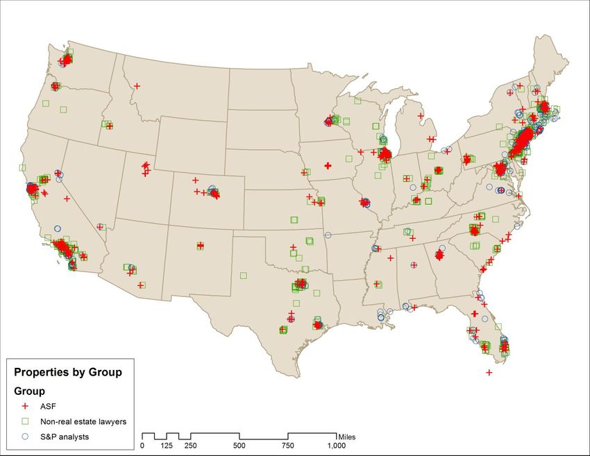
Figure 2 presents a map of properties in our sample. The most represented areas for all
groups are the Middle Atlantic (NJ-NY-PA) and Pacific areas (dominated by California). The
New York combined statistical area (roughly the NJ-NY-CT tri-state metro area plus Pike
County, PA) is the most prominent metro area, followed by Southern California (Los Angeles
plus San Diego). Equity analysts tend to be concentrated more in New York. Table B2 in
Appendix B presents the geographical distribution in detail.
Table 2, Panel B summarizes the results of our income matching procedure. For the
securitization sample, we have mortgage and census tract information for 292 purchases out of
388 we observe from 2000-2010. Of these, 200 are matched, an unconditional success rate of
52%; for the equity analyst and lawyer groups, this rate is 52% and 45%, respectively. Over the
entire 2000-2010 period, the average income level at purchase was $345K for the securitization
sample, $409K for the equity analyst sample, and $186K for the lawyers. All income figures are
reported in 2006 dollars adjusted using the Consumer Price Index (CPI) All Items series as of the
end of December 2006.
There are a number of caveats in analyzing our observed income figures. First, one concern
is that these numbers appear a bit too “small” relative to what is commonly perceived as finance
industry pay. The income reported in HMDA represents income used by the bank to underwrite
the loan, which may often include only taxable income provided by the mortgage applicant and
is thus likely downward biased. Forms of compensation not taxable during the year, such as
employee stock option grants, would not be included. What matters for our subsequent analysis
is whether the time variation in the bias is homogeneous across our samples. If there is a
constant amount of underreporting within each group across time, comparing the time-variation
in income across groups is a valid exercise. However, if the amount of underreporting varies
15
There are a small number of properties for which we have no purchase date. A missing purchase price reflects
missing data, which we deal with below. There are a substantial number of properties with either no sale date or a
sale date after December 31, 2010; these are homes that were still owned as of that date.
19across time, the bias becomes problematic. Second, even if this reporting issue were not present,
observed income levels are not unbiased representations of the true distribution of underlying
income because we only observe income at purchase, and not income in other years (and for
non-purchasers). Finally, our analysis does not represent income of the same people at repeat
purchases, and the small sample size makes it difficult to draw definitive conclusions. However,
with these caveats in mind, we view this as a useful descriptive exercise that allows us to
compare the time-variation in purchase income across groups and assess whether the
securitization and equity analyst groups received similar shocks across time.
Table 3 breaks down average income observed at purchase into three bins, corresponding to
the pre-housing boom (2000-2003), housing boom (2004-2006), and housing bust (2007-2010).16
Our securitization agents received large income shocks from the pre-boom to the boom period,
with average income rising by $145K, over 50% of average pre-boom income. Equity analysts
also received income shocks, with average income at purchase rising by $51K. Median incomes
rose for both groups by more comparable magnitudes. These results are roughly consistent with
our initial hypothesis that the two finance industry groups received positive income shocks,
although securitization agents received a slightly larger average shock.
Table 4 summarizes transaction prices each year. Through 2004, the average purchase price
for securitization agents increases from $525K to $944K in 2004, declining thereafter. Equity
analysts’ purchase prices are higher than the securitization group on average, even before the
housing boom; the average purchase price in 2000 was $850K. Average purchase prices for
lawyers began with $454K in 2000, rising slightly to a peak of $583K in 2005 and falling
slightly thereafter.
Examining annual purchase and sale activity is reduced form in that it masks the underlying
choices of individuals. Table 5 breaks down purchases and sales by transaction type over the
entire period 2000-2010. The number of purchase transactions exceeds the number of sale
transactions, since a number of people may be still living in homes they purchased. The most
common purchase type observed is buying a first home. Buying a second home and swapping a
16
Because we are interested in average income per person, we first average within person over purchases to obtain a
person-level average income for the period before averaging over people in each period.
20home for a more expensive one are the next most common purchases. Among sales, a sale
involved in any type of swap is the most common transaction.17
4. Empirical Results
4.1. Were securitization agents more aware of the bubble?
Figure 3 plots the housing stock of each group through time as a ratio relative to the housing
stock for each group at the end of 1999. Both the securitization agent and equity analyst groups
nearly doubled their stock of houses through 2007, with a decline through the end of 2009 for the
securitization group before rising again. This already suggests that there is little evidence of the
securitization agent sample being cautious as a group, as their housing stock if anything grew the
most aggressively through time.
To more formally analyze the inside job hypothesis, we first examine whether securitization
agents divested houses in advance of the housing crash. This is a necessary condition for timing
the bubble successfully. Table 6 presents the divestitures per person per year for each group
through time. These intensities are also plotted in Figure 4. The raw divestiture intensities for
the securitization agent sample are, if anything, lower than the divestiture rates of equity analysts
and lawyers during the bubble period. On an unadjusted basis, the rate of divestiture is
qualitatively lower for the securitization agent sample compared to both of the equity analysts
and lawyers in every year from 2003-2006, with the exception of 2004, and higher during the
bust period, 2007-2009.18
To account for heterogeneity in the age profiles of each group, we compute regression-
adjusted differences in intensities. We do this by constructing a strongly-balanced person-year
panel that tracks the number of divestitures each year for each person, including zero if no
17
The total number of swap sales and swap purchases over 2000-2010 may not exactly match as there may be
corresponding swap legs six months before and after this period. In this case, there was one swap where the sale leg
was executed in 2000 while the purchase leg was executed in 1999 for securitization agents, and vice versa for one
swap pair of lawyers.
18
The raw number of divestitures each year may be read off by multiplying the intensity in a given year from Table
6 by the number of homeowners in that year given by Table B3 in Appendix B. For example, in 2008, there were
eighteen divestitures (0.065 times 276) in the securitization sample. In contrast to our regression-adjusted
differences, we do not condition on having age information when reporting these raw intensities.
21divestiture was observed. We then estimate the following equation for each possible pairing of
the securitization group with other groups using OLS:
[ ]
∑
The variable is the number of divestitures for individual i in year t,
represents an indicator for whether individual i is part of our securitization
agent sample, represents an indicator for whether individual i is part of age group j in
year t (where eight age brackets are defined according to Table 1, Panel B, and one age group is
excluded), and represents whether individual i was also a multi-homeowner in year t.
We use indicators for age brackets instead of a polynomial specification for age as it makes the
regression easily interpretable as a difference in means. In each year t, we condition the sample
such that only the adjusted homeowners for year t (i.e., those who started year t as homeowners
or became a homeowner during year t) are included in the estimation. The coefficients are
thus the annual difference in average divestitures per person within the homeowner category
across samples, adjusted for these age and multi-homeownership factors. We cluster standard
errors by person.19
Table 6 presents these regression-adjusted differences. Rates of divestiture are statistically
similar in every year of the sample. Economically, divestiture rates are lower for the
securitization group in 2006 and higher in 2007-2009. Overall, there is little evidence that
suggests people in our securitization agent sample sold homes more aggressively prior to the
peak of the housing bubble relative to either equity analysts or lawyers.
19
The effective sample size (number of people contributing to the variation) of this estimation will be the total
number of people who we ever observed as adjusted homeowners during the 2000-2010 period for whom we have
age information across these two groups. This may be read off from the last row of Table B3, Panel B. For
example, when estimating equation (1) for the securitization sample and the equity analyst sample, the number of
people will be 517 (292 plus 225). The number of homeowners contributing to the variation each year may
similarly be read off from the same table, which lists the number of homeowners and non-homeowners each year
with age information. For example, when estimating (1) for the securitization agent and equity sample, the number
of people observed in 2000 is 343 (195 plus 148).
22You can also read