Grazing-related nitrous oxide emissions: from patch scale to field scale - Biogeosciences
←
→
Page content transcription
If your browser does not render page correctly, please read the page content below
Biogeosciences, 16, 1685–1703, 2019
https://doi.org/10.5194/bg-16-1685-2019
© Author(s) 2019. This work is distributed under
the Creative Commons Attribution 4.0 License.

Grazing-related nitrous oxide emissions:
from patch scale to field scale
Karl Voglmeier1,2 , Johan Six2 , Markus Jocher1 , and Christof Ammann1
1 Climate   and Agriculture Group, Agroscope, Zürich, 8046, Switzerland
2 Department   of Environmental Systems Science, ETH Zurich, Zürich, 8092, Switzerland

Correspondence: Christof Ammann (christof.ammann@agroscope.admin.ch)

Received: 2 October 2018 – Discussion started: 29 October 2018
Revised: 22 February 2019 – Accepted: 15 March 2019 – Published: 25 April 2019

Abstract. Grazed pastures are strong sources of the green-        system M and 0.83 ± 0.29 % for system G. These EF val-
house gas nitrous oxide (N2 O). The quantification of N2 O        ues were thus significantly smaller compared to the default
emissions is challenging due to the strong spatial and tem-       EF of 2 % provided by the IPCC guidelines for cattle excreta
poral variabilities of the emission sources and so N2 O emis-     deposited on pasture. The measurements showed that urine
sion estimates are very uncertain. This study presents N2 O       patch emission dominated the field-scale fluxes (57 %), fol-
emission measurements from two grazing systems in western         lowed by significant background emissions (38 %), and only
Switzerland over the grazing season of 2016. The 12 dairy         a small contribution of dung patch emission (5 %). The re-
cows of each herd were kept in an intensive rotational graz-      sulting source-specific EFs exhibited a clear difference be-
ing management. The diet for the two herds of cows con-           tween urine (1.12 ± 0.43 %) and dung (0.16 ± 0.06 %), sup-
sisted of different protein-to-energy ratios (system G: grass     porting a disaggregation of the grazing-related EFs by exc-
only diet; system M: grass with additional maize silage) re-      reta type in emission inventories. The study also highlights
sulting in different nitrogen (N) excretion rates. The N in the   the advantage of a N-optimized diet, which resulted in re-
excretion was estimated by calculating the animal nitrogen        duced N2 O emissions from animal excreta.
budget taking into account the measurements of feed intake,
milk yield, and body weight of the cow herds. Directly after
the rotational grazing phases, background and urine patches
were identified based on soil electric conductivity measure-      1   Introduction
ments while fresh dung patches were identified visually. The
magnitude and temporal pattern of these different emission        Nitrous oxide (N2 O) is a strong greenhouse gas (GHG) with
sources were measured with a fast-box (FB) chamber and the        a 265 times stronger warming potential compared to CO2 on
field-scale fluxes were quantified using two eddy covariance      a mass basis (IPCC, 2014). Typically an inert gas in the tro-
(EC) systems. The FB measurements were finally upscaled           posphere, N2 O has a strong potential to destroy the ozone
to the field level and compared to the EC measurements for        layer in the stratosphere (Portmann et al., 2012). The largest
quality control by using EC footprint estimates of a back-        share of N2 O emissions are attributed to nitrogen (N) fertil-
ward Lagrangian stochastic dispersion model. The compari-         ization in the agricultural sector, but livestock grazing, espe-
son between the two grazing systems was performed during          cially by cows, can also lead to significant direct and indi-
emission periods that were not influenced by fertilizer appli-    rect N2 O emissions due to excreta from the animals (Luo et
cations. This allowed the calculation of the excreta-related      al., 2017; Reay et al., 2012). The nitrogen deposited by ani-
N2 O emissions per cow and grazing hour and resulted in con-      mal excreta often exceeds the N applied by fertilizer (Aarons
siderably higher emissions for system G compared to system        et al., 2017). The available reactive N is used by micro-
M. Relating the found emissions to the excreta N resulted in      bial nitrification and denitrification processes where signif-
excreta-related emission factors (EFs) of 0.74 ± 0.26 % for       icant amounts of N2 O can be produced (Selbie et al., 2015).
                                                                  A nonlinear response of N2 O emissions to N loading has

Published by Copernicus Publications on behalf of the European Geosciences Union.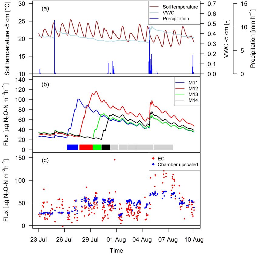
1686                            K. Voglmeier et al.: Grazing-related nitrous oxide emissions: from patch scale to field scale

been shown previously (Cardenas et al., 2010), and urine             were often performed on manually applied urine and dung
patches of cattle have exceptionally high N loading rates (up        patches (Bell et al., 2015; Cai and Akiyama, 2016). Addition-
to 2000 kg N ha−1 ), making them especially prone to high            ally, due to the strong heterogeneity of the emissions from
N2 O losses (Selbie et al., 2015).                                   a pasture (Cowan et al., 2015; Flechard et al., 2007) cham-
   For inventories and live cycle assessments, the magnitude         ber techniques are not ideal to compute field-scale emis-
of the N2 O emissions is usually calculated by applying emis-        sions for grazing systems. The eddy covariance (EC) method
sion factors (EFs) related to the magnitude of N inputs to the       overcomes this problem by integrating over multiple emis-
agricultural fields (EF = emitted N2 O-N/N input). Accord-           sion sources over a larger spatial domain. The EC technique
ing to the guidelines of the Intergovernmental Panel on Cli-         was already applied successfully to quantify N2 O emissions
mate Change (IPCC, 2006) for national emission reporting, a          from pastures and grasslands (Jones et al., 2011). Some stud-
separation is made between (i) emissions related to excreta N        ies also tried to compare different systems (e.g., intensive
deposited by the grazing animals and (ii) emissions related to       – extensive, different crops, land/lake) with one EC tower
fertilizer applications and other N inputs. While for fertilizer-    (e.g., Biermann et al., 2014; Fuchs et al., 2018) by partition-
induced N2 O emissions, a default value of 1 % is proposed           ing the fluxes based on wind direction and system geometry,
by IPCC (2006), the default EF related to excreta of grazing         but typically one tower for each system is preferable. In or-
cattle (denoted as EF3PRP,CPP ) is 2 %. Most countries includ-       der to understand and quantify the emissions of a pasture,
ing Switzerland presently use these default values. However,         the combined approach of EC measurements and chambers
the default EF3PRP,CPP value often overestimates observed            is regarded as the best solution (Cowan et al., 2015). The
pasture emissions (Bell et al., 2015; Chadwick et al., 2018)         EC systems can be used to quantify the field-scale emissions
and does not take into account country-specific conditions           while the chamber approach can be used to estimate the con-
(climate, soil, management). Therefore, some countries have          tributions from single emission sources (urine patches, dung
developed a country-specific EF (e.g., New Zealand; Saggar           patches, and other “background” areas).
et al., 2015) which is still lacking for Switzerland. Addition-         In our experiment, we measured N2 O emissions from two
ally, it has been shown that separate EFs for urine and dung         neighboring pastures simultaneously with the EC method
might be beneficial in describing the emissions and under-           over a full grazing season. The two pastures differed in the
standing the contributions of the different emission sources         energy-to-protein balance of the cows’ diet. The small-scale
on a pasture (Bell et al., 2015). A better understanding of the      fluxes were quantified with a fast-box chamber and upscaled
individual contributions would also be very helpful to reduce        to match the EC flux footprints for comparison. Further
the emissions, as dietary changes, for example, typically af-        on, we computed the contribution of the different emission
fect the excreted urine N, which is mainly responsible for the       sources to the overall pasture emissions. The results were
high N2 O emission associated with excreta (Dijkstra et al.,         compared to default values provided by IPCC and other liter-
2013). However, the range and thus the uncertainty of spe-           ature values. The main goal of the study was to quantify the
cific urine EFs is rather large (0 %–14 %, n = 40) as shown          excreta-related emission and the corresponding EF for real
by Selbie et al. (2015) based on a survey of literature reports.     grazing systems and to analyze the specific contributions of
Many of those studies measured the emissions on artificially         dung and urine patches.
applied urine or under laboratory conditions, making these
results questionable with regard to the applicability within
greenhouse gas inventories.                                          2     Material and methods
   The efficient use of fed N is essential to reduce the emis-
sions associated with animal excreta. Studies have shown             2.1    Experimental site
that an optimized feeding strategy can lead to less N excreted
by the animals (e.g., Arriaga et al., 2010; Dijkstra et al., 2013;   The experiment was conducted at the research farm Agro-
Yan et al., 2006). For this purpose, forage with a low N con-        scope Posieux in the Prealps of Switzerland in the canton
tent (e.g., maize) can be used as a supplement to N-rich grass       of Fribourg (46◦ 460 0400 N, 7◦ 060 2800 E) during the grazing
and this subsequently leads to less N in the excreta, mainly         season of 2016 and has already been described in detail by
in the form of less urine N. A lower amount of N input to            Voglmeier et al. (2018). The farm is located at an elevation
the pasture is supposed to produce less N2 O emissions, but          of 642 m with an annual average temperature of 8.7 ◦ C and
corresponding emission experiments under real grazing con-           a mean annual precipitation sum of 1075 mm (MeteoSwiss,
ditions for a full season, to our knowledge, have not been           2018). The soil consisted mainly of a stagnic Anthrosol with
reported hitherto.                                                   a loamy texture (see Table 1). Soil profile samples for anal-
   Historically, most studies used static chambers to quan-          ysis of texture and other soil characteristics were taken at
tify N2 O emissions (Flechard et al., 2007). Chamber mea-            four locations on the pasture in 2013 and 2016. The vege-
surements are ideal to quantify emissions on a small spatial         tation consisted of a grass–clover mixture typical for Swiss
scale and to attribute the measured fluxes to certain emis-          pastures (78 ± 12 % grasses and 15 ± 10 % legumes; main
sion drivers, but for excreta emissions these measurements           species: Lolium perenne and Trifolium repens, 10 sampling

Biogeosciences, 16, 1685–1703, 2019                                                      www.biogeosciences.net/16/1685/2019/

K. Voglmeier et al.: Grazing-related nitrous oxide emissions: from patch scale to field scale                                  1687

Table 1. Near-surface soil parameters (5–10 cm depth) averaged      Table 2. Measured averages ± standard deviation of observed cow
over four locations on the pasture. The measurements are given as   properties (ECM: energy corrected milk) and feed protein contents
mean ±1 standard deviation.                                         used by the dairy cow nitrogen budget approach for both pasture
                                                                    systems during the grazing season 2016.
              Parameter                              Value
                                                                      Input parameter (units)               System M     System G
              Pore volume (%)                        57 ± 4
              Bulk density (g cm−3 )            1.09 ± 0.11           Number of cows                               12            12
              pH (–)                              6.0 ± 0.3           Milk yield, ECM (kg cow−1 day−1 )    25.1 ± 2.9    24.2 ± 3.7
              Sand (%)                           42.6 ± 2.5           Animal weight (kg)                    633 ± 14      633 ± 10
              Clay (%)                           18.7 ± 1.7           Grass crude protein (g kg-DM−1 )      195 ± 23      196 ± 23
              Silt (%)                           33.0 ± 1.3           Maize crude protein (g kg-DM−1 )         84 ± 8           n/a
              Soil organic matter (%)             5.7 ± 0.3
              Total N (%)∗                      0.38 ± 0.03         n/a – not applicable
              Total C (%)∗                      3.76 ± 0.20
            ∗ Measured at a depth of 0–10 cm.
                                                                    spent a longer time in the barn during daytime (up to 6 h; see
                                                                    Fig. 2c) mainly due to high air temperatures and to a minor
                                                                    degree to additional experiments of other research groups.
times between May and September). After the last renova-            Heavy rain events in June led to very wet soil conditions,
tion treatment in 2007 the field had been used as an inten-         which prevented grazing between 8 June and 4 July and ne-
sive pasture for cattle grazing with occasional grass cuts for      cessitated a grass cut on 22 and 27 June (Fig. 2c).
maintaining a homogenous sward. In addition to the N input
through excreta from the grazing animals, N had been ap-            2.3     N input to the pasture
plied through fertilizer at a rate of about 120 kg N ha−1 per
year between 2007 and 2015.                                         During the grazing season, N input to the pasture mainly
                                                                    occurred in the form of excreta of the grazing animals and
2.2   Experimental design                                           to a lesser extent as mineral fertilizer (Fig. 2d). The min-
                                                                    eral fertilizer was ammonium nitrate (28 kg ha−1 ) applied at
The experiment took place at a 5.5 ha pasture, which was di-        the end of June and urea (42 kg ha−1 ) with a split applica-
vided into two separate systems differing in feeding strat-         tion between the middle of August (western paddocks X.11–
egy of the 12 cows per system (Fig. 1a). The northern sys-          X.16) and early September (eastern paddocks X.21–X.25)
tem (system M) represented a N-optimized feeding option             due to concurrent grazing. In the present study we focus on
where the diet of the cows consisted of grass with additional       the N input by grazing excreta and their effect on N2 O emis-
maize silage (roughly 20 % of the dry matter intake, DMI,           sions. The comparison between the field-scale EC method
fed in barn during milking periods) resulting in a demand-          and the small-scale chamber measurements also required es-
optimized protein content in the diet (Arriaga et al., 2010;        timates of the number of dung and urine patches on the pas-
Yan et al., 2006). This was supposed to reduce the excreta N        ture. These numbers were calculated as described in Sect. 2.7
input to the pasture. The southern system (system G) repre-         based on the excreted N amounts. N excretion cannot easily
sented a full grazing regime with no additional forage, which       be measured in the field, but it can be calculated based on
resulted in a considerable protein surplus (see Table 2). Both      the energy demand of the cows and measured N in feeds and
systems were managed as a rotational grazing system with            products (e.g., milk, body weight gain). We followed the ap-
11 paddocks (Fig. 1a) resulting in a typical rotation period        proach described by Felber et al. (2016) to calculate the en-
of about 20 days. The size of the paddocks was adjusted for         ergy and N flows of the dairy cows in the experiment and to
the different feeding strategies and resulted in typical sizes      calculate daily values of excreted N per cow. Input param-
of 1700 m2 for system M and 2200 m2 for system G. The               eters to the budget calculation were daily measurements of
rotation of both systems was managed synchronously with             milk yield, milk N content, and body weight gain as well as
a new rotation starting on the westerly paddocks (X.11 to           seasonal measurements of protein content of the grass (eight
X.16 with X indicating both systems) followed by the east-          times between end of April and end of September) and of the
erly ones (X.21 to X.25).                                           maize silage (three times between beginning of May and be-
   Grazing on the paddocks started with intermittent grazing        ginning of September). The breakdown of the excreted N in
phases in March and ended in early November with the main           urine and dung was based on work by Bracher et al. (2011).
grazing season being between the end of April and early Oc-         For further details see Voglmeier et al. (2018), where the cor-
tober. During this time period eight full rotations took place.     responding uncertainty of the total N and urine/dung N was
The cows typically spent 18 to 20 h per day on the pasture          estimated to be 15 % (2σ ) for the same experiment. Seasonal
and were brought to the barn twice a day (around 05:00 and          statistics of the input variables are given in Table 2.
17:00 LT) for milking. However, in July and August the cows

www.biogeosciences.net/16/1685/2019/                                                        Biogeosciences, 16, 1685–1703, 2019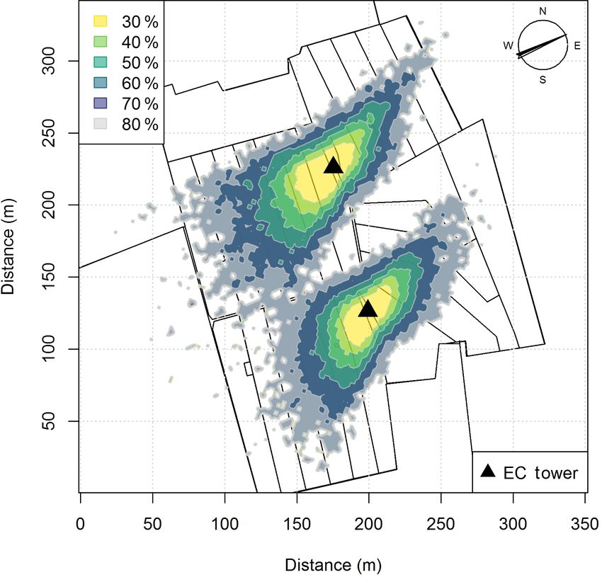
1688                             K. Voglmeier et al.: Grazing-related nitrous oxide emissions: from patch scale to field scale

Figure 1. (a) Measurement site with the pastures for the two herds (blue: grass diet with additional maize silage; green: full grazing regime;
grey: optional pasture areas) and the division into the paddocks (M.11–M.25, G.11–G.25). Additionally the location of the two EC towers
(triangles) and the area of the chamber measurements (red dashed rectangles) are shown. (b) Wind distribution for the northern sonic
anemometer with the corresponding sector contributions (black dotted circles) for the period May–October 2016. The areas A and B indicate
wind sectors from which advection from nearby farm building can occur. The wind distribution was overlaid on a Google Earth image of the
experimental area (map data: Google, DigitalGlobe).

2.4     Small-scale flux measurements                                    2.4.2    Fast-box measurements

2.4.1    Excreta detection
                                                                         Small-scale emissions from urine and dung patches as well
The localization of fresh dung and urine patches was es-                 as background pasture areas were measured with a fast-box
sential in this study to measure N2 O emissions attributable             (FB) chamber (Hensen et al., 2006). The measurements took
to specific excreta sources. Intensive observation areas of              place on the paddocks X.11 and X.21 (Fig. 1a) between the
10 m × 10 m or 15 m × 15 m close to both EC towers in the                beginning of July and middle of October and were therefore
paddocks X.11 and X.21, respectively (see Fig. 1a) were se-              taken mainly during dry soil conditions (Fig. 2a, periods with
lected. Within these areas fresh dung and urine patches were             VWC < 0.4). Measurements usually started after the excre-
mapped typically 1–3 days after grazing of the respective                tion detection (Sect. 2.4.1) and about 1–2 days after the end
paddock. Dung pats were mapped visually and labeled for                  of grazing (EOG). The age of the excreta patches is impor-
subsequent chamber measurements. For urine patches a di-                 tant for the interpretation of the measured fluxes. However,
rect visual identification was not possible. Bates et al. (2015)         the exact determination of the excreta age was not possible.
demonstrated the ability of surface-soil electrical conduc-              Thus, the time since EOG was used as excreta age for each
tivity measurements to detect urine patches. Using this ap-              FB measurement. The potential age variability of a single
proach we mounted a soil probe (GS3, Meter Group, US; for                excreta patch resulted from the sojourn time of the cows on
soil moisture, temperature, and electrical conductivity mea-             the paddock, which typically was in the range of 1–1.5 days.
surements) on a handheld stick and mapped the intensive                     The manually operated opaque 0.8 m × 0.8 m × 0.5 m box
observation area on a 25 cm grid (Fig. 3). Based on pre-                 was connected to a fast response quantum cascade laser
experimental tests, areas with conductivity values below a               analyzer (QCL, Aerodyne Research Inc.) that was also
threshold of 0.15 mS cm−1 (dark blue areas in Fig. 3a) were              used for the EC system on the respective field (see below
considered background without recent influence of excreta.               Sect. 2.5.1). The sample air was drawn continuously from
Spots with a conductivity above the threshold were marked                the FB headspace through a 40 m 1/400 polyamide (PA) tube
as possible urine patches for the chamber measurements.                  to the analyzer, allowing measurements within a radius of
Time series of electrical conductivity measurements (Fig. 3b)            about 35 m on the paddocks X.11 and X.21 (see Fig. 1).
on manually applied urine patches in 2017 illustrate the long-           The sample flow rate Q was typically around 8 L min−1 . The
term effect and demonstrate the possibility to distinguish be-           box was modified by using a defined vent to ambient air
tween background areas and urine patches more than 10 days               through a tube of 4 cm in diameter and 1 m in length. The
after the application of urine.                                          inlet of the vent tube was packed with a foam material over
                                                                         a length of 10 cm to avoid uncontrolled air exchange due to
                                                                         wind-induced pressure fluctuations. The chamber was also
                                                                         equipped with a GMP343 CO2 probe (Vaisala, FI) to mea-

Biogeosciences, 16, 1685–1703, 2019                                                             www.biogeosciences.net/16/1685/2019/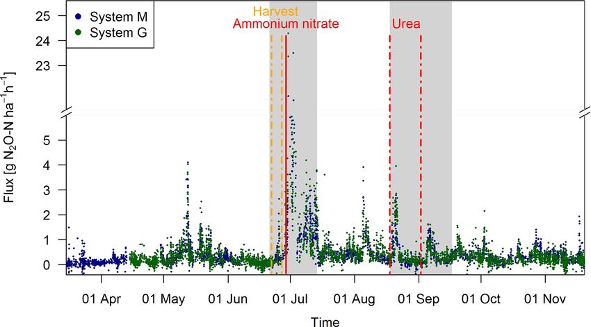
K. Voglmeier et al.: Grazing-related nitrous oxide emissions: from patch scale to field scale 1689
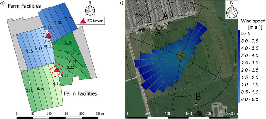
Figure 2. Time series of (a) daily averaged soil temperature and moisture at a depth of 5 cm measured at system M (solid lines) and spread
of the four measurement locations, (b) daily air temperature at 2 m above ground and precipitation at the measurement site, and (c) grazing
duration on the single paddocks of the pasture (X: both pasture systems M and G) for the study year 2016. The dashed vertical orange lines
indicate the harvest event (split between X.11–X.16 and X.21–X.25) (d) N input to system M during the main grazing season in 2016.
Fertilizer was applied two times (vertical red lines). The second application (dashed lines) in August was split in two parts due to concurrent
rotational grazing. The grey shaded areas indicate time periods influenced by fertilization or harvest events as explained in Sect. 2.5.2.
sure the soil respiration, which was used for quality control
purposes (Sect. 2.4.3). The increase in N2 O concentration af- A · FCham Q
ter placing the chamber on the soil with a flux FCham was C (t) = 1 − e− V ·t + Cbg . (1b)
Q
recorded every 3 s for a time period of about 90 s (taking into
account the time delay due to tube sampling). The inflow of For small values of the exponent Q/V · t (slow chamber vol-
the background concentration Cbg into the chamber volume ume exchange of about 40 min and short measurement time)
V (with area A) through the vent led to lower measured con- as characteristic for the present fast-box measurements, the
centration values C. This can be described by the following entire bracket term can be linearized with a series expansion
differential equation for the chamber headspace concentra- to (Q/V · t). Inserting the resulting function for C(t) into
tion C(t): Eq. (1a) yields
δC
δC Q
V = A · FCham − Q C − Cbg . (1a) V = A · FCham 1 + t . (1c)
δt δt V
This is a combination of the two equations for static cham- With the FB dimensions and sampling flow rate as given
bers (right-hand term = 0) and for the dynamic chamber (left- above and a maximum accumulation time t ≤ 2 min, the de-
hand term = 0). Solving of the equation yields the explicit viation from the ideal linear increase in a fully closed static
time function chamber was ≤ 5 %. The flux was finally calculated by using
www.biogeosciences.net/16/1685/2019/ Biogeosciences, 16, 1685–1703, 2019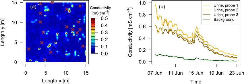
1690                             K. Voglmeier et al.: Grazing-related nitrous oxide emissions: from patch scale to field scale

the HMR package (Pedersen et al., 2010), which uses linear             abled a good footprint coverage (Fig. 4, Sect. 2.5.4) of both
and nonlinear regression to fit the measured concentration             fields and allowed the measurement of field-scale fluxes of
values. The uncertainty of an individual box measurement is            both systems.
estimated to be around 20 % (Hensen et al., 2006).                        The two EC systems were identically equipped with an ul-
   In order to relate the measured fluxes to environmental             trasonic anemometer–thermometer (further on named sonic,
driving parameters the following sensors were placed inside            HS-50, Gill Instruments Ltd., UK) to quantify the turbu-
on the chamber: a thermocouple (type K) for air temper-                lent mixing by measuring the three-dimensional wind ve-
ature measurement within the chamber, a GS3 probe (see                 locity (u, v, w) and air temperature. Dry air mixing ratios
Sect. 2.4.1) for soil moisture, soil temperature, and soil con-        of N2 O were measured with closed-path quantum cascade
ductivity measurements (ca. 0–5 cm depth), and an ML3                  laser spectrometers (QCL, QC-TILDAS, Aerodyne Research
ThetaProbe (Delta-T Devices Ltd., UK) for soil moisture and            Inc.) that analyzed air samples drawn through a 25 m PA tube
soil temperature observations (ca. 0–10 cm depth). All mea-            (inner diameter 6 mm) by a vacuum pump (Bluffton Mo-
sured data values were stored on a data logger mounted on              tor Works, flow rate ca. 13 L min−1 ). One filter at the inlet
top of the box and transferred to a computer in the nearby             (AcroPak, Pall Corporation, 0.2 µm) and one before the in-
shelter or trailer. A customized LabVIEW (National Instru-             strument (Midisart 2000, Sartorius Stedim Biotech GmbH,
ments, US) program allowed for online inspection of all mea-           0.2 µm) were used for each system to filter out particles.
sured data values including the gas concentrations.                    The distance of the inlets of the QCL from the center of
                                                                       the sonic head were around 20 cm and the QCL instruments
2.4.3    Quality control and system comparison                         were placed in a temperature-controlled environment (trailer
                                                                       at system M, shelter at system G) about 20 m north (system
FB fluxes were selected for post-processing after fulfilling           M) or south (system G) of the EC towers.
certain quality criteria. In a first step, the R 2 value of any flux      The sample frequency of the EC system was 10 Hz. A cus-
calculation had to exceed 0.9 (e.g., for N2 O flux the R 2 value       tomized LabVIEW (National Instruments, US) program was
of N2 O, CH4 , or CO2 had to exceed 0.9). For urine patches,           used to combine the data strings of the individual instruments
the soil conductivity had to exceed 0.25 mS cm−1 at the be-            and store them as binary raw data for offline analyses. Addi-
ginning of the measurements (see also Fig. 3b) in order to ex-         tionally the program visualized the measurements and fluxes
clude possible old urine patches (of previous management ro-           of the N2 O concentrations and fluxes, calculated with an on-
tations). Presumable old patches were therefore rejected for           line flux calculation. The program also allowed us to check
further processing. Background fluxes were removed from                the EC system by remote access.
further processing if the flux value exceeded 40 µg m−2 h−1
(= 4 × median value) to ensure that undetected urine patches           2.5.2   Flux calculation
at the chamber surroundings did not influence the flux mea-
surements. Finally, 360 and 293 flux measurements met the              A customized program written in the statistical software R
criteria on systems M and G, respectively. These measure-              (R Core Team, 2016) was used to calculate EC fluxes for
ments were composed of 238 background fluxes, 242 urine                30 min intervals (similar to Felber, 2015, and Felber et al.,
patch fluxes, and 173 dung fluxes.                                     2015). The program is based on Ammann et al. (2006, 2007).
   For a direct comparison of the FB measurements on the               In a first step, 10 Hz data outside a plausible physical range
two pasture systems, the fluxes obtained on the same day               were identified and replaced by a running mean filter with a
were ordered based on their magnitude for each system and              window size of 500 data points. In a next step, wind vector
source class. Due to the synchronous grazing regime, the               components were rotated into the mean wind direction using
fluxes represented the same excreta age (e.g., on day 3 af-            the double coordinate rotation technique (Kaimal and Finni-
ter EOG). However, synchronous FB measurements on both                 gan, 1994), and concentration values were subject to linear
systems were not always performed. Resulting numbers of                detrending within an averaging interval of 5 min.
data pairs are 46, 54, and 40 for background, urine, and dung             The EC flux is defined as the covariance of the vertical
fluxes, respectively.                                                  wind speed and the trace gas mixing ratio. Due to the long
                                                                       inlet tube the time series of the trace gas signals are delayed
2.5     Field-scale flux measurements                                  in relation to the wind measurements by a quasi-constant lag
                                                                       time of about 6 s for system M and 7 s for system G. Thus,
2.5.1    Eddy covariance system                                        the trace gas signals have to be shifted to obtain the correct
                                                                       covariance flux (Langford et al., 2015). In a pre-evaluation,
For field-scale flux measurements EC towers were installed             the “default lag” was determined as the most frequent posi-
in the middle of the two pasture fields to account for the pre-        tion of the maximum absolute value of the cross-covariance
dominant wind directions northeast and southwest (Fig. 1)              function over periods of weeks to months (depending on in-
and were fenced with a radius of 2–3 m to avoid unwanted               strument maintenance). Then it was checked for each half-
animal contact. The measurement height was 2 m, which en-              hour period whether the individual “dynamic” lag was within

Biogeosciences, 16, 1685–1703, 2019                                                        www.biogeosciences.net/16/1685/2019/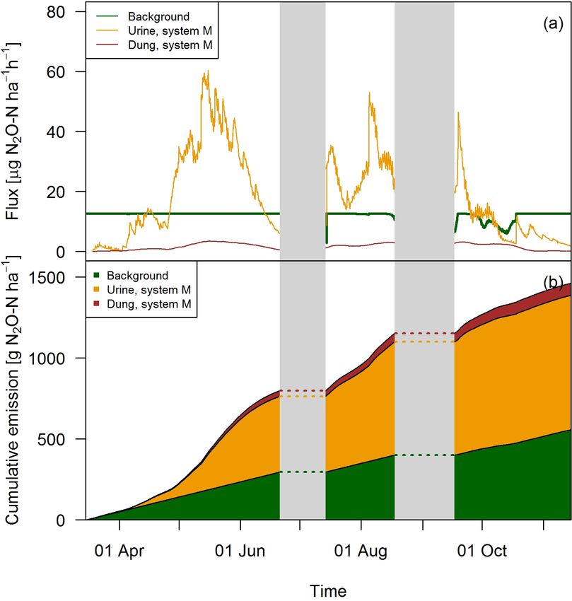
K. Voglmeier et al.: Grazing-related nitrous oxide emissions: from patch scale to field scale                                       1691

Figure 3. (a) Measured conductivity within a quadratic 15 m × 15 m intensive observation area on the 3 October 2016 in system G. High val-
ues (> 0.15 mS cm−1 ) indicate urine patch locations and brown crosses indicate observed dung pats. (b) Conductivity measured continuously
during a field experiment in 2017 with four GS3 sensors.

                                                                       were quantified using the “ogive” method where the damp-
                                                                       ing factor was calculated by fitting the normalized cumula-
                                                                       tive co-spectrum of N2 O to the one of the sensible heat at a
                                                                       frequency of 0.065 Hz. In a post-processing step, these half-
                                                                       hourly damping factors were filtered for favorable conditions
                                                                       e.g., low noise level of the ogive and the flux. The selected
                                                                       values were used to compute a damping function dependent
                                                                       on wind speed and stability which was finally used to es-
                                                                       timate the damping factor. Depending mainly on the wind
                                                                       speed, a damping effect of 10 %–30 % was found and cor-
                                                                       rected for.
                                                                          EC fluxes were measured continuously over the grazing
                                                                       season. Since the present study is focused on N2 O emissions
                                                                       from grazing, time periods with strong influence of N2 O
                                                                       emissions from fertilization and harvest events (see Fig. 2c–
                                                                       d) were excluded for computation of cumulative emissions
                                                                       and for comparisons between field-scale and small-scale
                                                                       measurements. These exclusion periods were limited to the
                                                                       15 days following fertilization or harvest and led to a rejec-
                                                                       tion of 47 days during the grazing season. The criterion is
Figure 4. Footprint climatology for both EC towers averaged for the    based on observed EC fluxes (Sect. 3.1) and is in accordance
time period between 15 March and 15 November 2016. The legend          with Jones et al. (2011). The time period used for calculation
values indicate the percentage of the total footprint weight.          of the cumulative grazing emissions is further on defined as
                                                                       grazing-only periods (GOPs) and accumulated to 198 days.

a time window of 0.61 s around the default lag. If this was the        2.5.3   Quality control and gap filling
case, the dynamic lag was used, otherwise the default lag was
used. In order to minimize the effect of nonstationarities in          EC flux measurements are subject to different sources of
the time series, the 30 min flux was finally calculated as the         measurement problems and quality issues, which often re-
average over six 5 min subinterval flux values. This caused a          sult in data loss or data rejection. These sources can be in-
minor low-frequency spectral loss (1 %–5 %) that was quan-             strument specific like power failures or malfunctioning, en-
tified (and corrected for) using Kaimal cospectra and the the-         vironmental driven like measurements under nonideal condi-
oretical transfer function for block averaging.                        tions (e.g., low turbulence), or a combination of both (Papale,
    The fluxes measured by EC systems are also subject to              2012). Power outage, instrument maintenance (only on sys-
different high-frequency losses due to sensor separation and           tem M), and delayed installation (only on system G) led to
in case of N2 O air transport through the inlet tubes (Foken           data losses during the GOP of 12 % and 17 % for systems M
et al., 2012). These damping effects can lead to a significant         and G, respectively. Data rejection due to low friction veloc-
underestimation of the flux and must be corrected. Based on            ity (u∗ < 0.07 m s−1 ) and large vertical tilt angle (−2 to 6◦ )
Ammann et al. (2006) the half-hourly high-frequency losses             of the wind vector led to a further data loss of about 35 %.

www.biogeosciences.net/16/1685/2019/                                                            Biogeosciences, 16, 1685–1703, 2019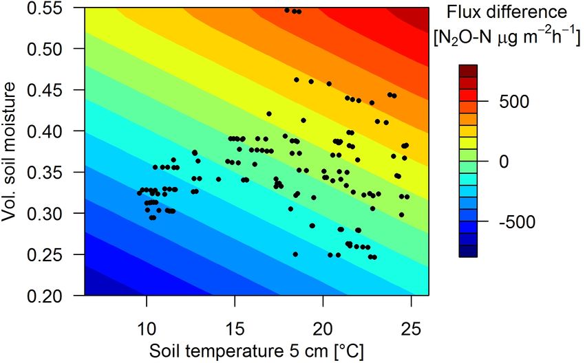
1692                           K. Voglmeier et al.: Grazing-related nitrous oxide emissions: from patch scale to field scale

Because nonstationarity of the flux was already reduced by          2.5.4    Footprint modeling
the short averaging/detrending interval of 5 min, a quality se-
lection based on nonstationarity (Foken et al., 2012) had little    EC measurements yield a spatially integrated flux over a cer-
effect and was therefore not used here. Additional rejection        tain area represented by the flux footprint (Schmid, 2002). In
of wind sectors influenced by the farm facilities, trailer, or      the present study, this footprint typically extends over multi-
shelter and to avoid cross-influences from the other pasture        ple grazing paddocks depending on wind direction and turbu-
system (wind dir = 280–25◦ and wind dir = 97–195◦ ) con-            lence intensity. Therefore quantitative footprint information
tributed to an overall data loss of 64 % and 69 % for systems       is needed for the comparison of the EC fluxes with the up-
M and G. The resulting occurrence of data gaps showed a di-         scaled FB measurements (Sect. 2.7), and the footprint has
urnal pattern with stronger data loss during the night, which       to be checked for the spatial dimension to be sure that the
was driven by the wind pattern with typically stronger wind         measured flux is mainly dominated by the area of the sys-
speeds during daytime and calm nights.                              tem and not contaminated by the neighboring systems (ei-
    The gaps in the flux time series needed to be filled in order   ther the other grazing system or fluxes originating from sur-
to compute cumulative sums over a certain period of time.           rounding fields). In this study an open-source version of a
However, no well-established reference method for the gap           backward Lagrangian stochastic dispersion footprint model
filling of N2 O fluxes exists to date. We followed the evalu-       (bLS) was used (Häni, 2017; Häni et al., 2018), based on
ation of Mishurov and Kiely (2011) and used a lookup ta-            Flesch et al. (2004). The flux-to-emission ratio is calculated
ble method (LUT) with three parameters: one for the pre-            following Eq. (2):
ceding cumulative rainfall of the last 12 h with three classes
                                                                             nj  i
(no rainfall, 0–2 mm, > 2 mm), one for the percentiles of           FEC   2 X   wini
                                                                        =            ,                                          (2)
the soil temperature at 5 cm depth during the GOP with              Ej    N i=1 woi
four classes (0–25th percentile, > 25th percentile–median,
> median–75th percentile, > 75th percentile), and one for           where FEC is the measured EC flux, Ej the surface emission
the footprint-weighted (Sect. 2.5.4) averaged cow density           of paddock (source area) j , N the total number of released
(cows ha−1 ) on the single paddocks over the preceding 5 days       particles, nj the number of touchdowns within paddock j ,
(0, 0–2, > 2 cows ha−1 ). To check the sensitivity towards dif-        i the vertical release velocity, and w i the touchdown ve-
                                                                    wini                                         o
ferent gap-filling methods, three other techniques were com-        locity of the particles.
pared to the LUT approach: (I) running mean with a vari-                In order to calculate the footprint for a 30 min period, N =
able filter window size and at least 12 values, (II) monthly        80 000 fluid particles were released backwards in time using
mean diurnal variation (MDV; see Zhao and Huang, 2015)              the wind and turbulence parameters calculated from the sonic
with a running half-hourly window size of five in order to          measurements of the EC systems. The systematic uncertainty
have more values during nighttime, and (III) seasonal MDV           of the bLS model was estimated to about 10 % (Flesch and
based on half-hourly values averaged over the whole grazing         Wilson, 2005; Wilson et al., 2013). The half-hourly footprint
season. Due to the delayed installation of the EC tower on          fractions of the individual paddocks were used to upscale the
the southern field, all values prior to 14 April on system G        small-scale measurements to the EC flux footprint (Sect. 2.7)
resulted from the gap-filling routine. The uncertainty of gap       for intercomparison of the two flux measurement methods.
filling for seasonal cumulative fluxes was estimated from the           In addition, the seasonally integrated footprint extension
standard deviations of monthly cumulative fluxes retrieved          was analyzed, taking into account the wind direction and u∗
with the different gap-filling methods during GOP, which re-        filtering as described in Sect. 2.5.3. The analysis showed a
sulted in an uncertainty of 14 % and 18 % for systems M and         distinct separation of the footprint distributions for the two
G, respectively (1σ ). It was assumed that this uncertainty re-     systems (Fig. 4) with only marginal contributions of the other
flects the sum of all important individual uncertainties of the     system (< 2.5 %). More than 80 % of the footprint contribu-
cumulative emissions (e.g., Sects. 3.3.1 and 4).                    tions were from the actual rotation area (without the optional
    The experimental setup was expected to result in very sim-      areas indicated in grey in Fig. 1a).
ilar systematic errors of the two EC systems; thus only the in-
dependent (or random) errors have to be considered for com-         2.6     Environmental parameters
paring the two neighboring systems (Ammann et al., 2009).
As the cumulative fluxes of both EC systems were by chance          In order to relate the measured fluxes to meteorological driv-
of similar magnitude (Sect. 3.1 and 3.3.1), the random uncer-       ing parameters, an automated weather station (with data log-
tainty of the cumulative EC fluxes was determined from the          ger CR10X, Campbell Scientific Ltd., UK) was installed at
differences between the cumulative monthly EC fluxes of the         the northern field next to the sonic. A WXT520 (Vaisala,
two towers and resulted in a relative uncertainty of 5 % (1σ ).     Vantaa, Finland) measured the wind speed, precipitation,
                                                                    temperature, and barometric pressure, and global radiation
                                                                    was measured with a pyranometer (CNR1, Kipp&Zonen,
                                                                    Delft, the Netherlands).

Biogeosciences, 16, 1685–1703, 2019                                                      www.biogeosciences.net/16/1685/2019/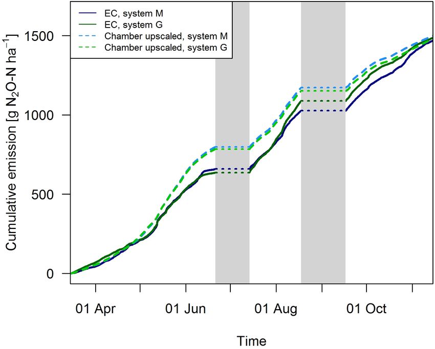
K. Voglmeier et al.: Grazing-related nitrous oxide emissions: from patch scale to field scale                                           1693

Figure 5. Flowchart of upscaling procedure to compare small-scale chamber fluxes with EC fluxes and to estimate the contribution of excreta
emissions to the overall pasture emission. Rectangular shapes indicate time series data and other data sets. Time series data with thin frames
have gaps whereas bold frames indicate complete data sets. The light blue color specifies N2 O flux data. Other shapes show operations (e.g.,
fit or gap-filling routines).

   Soil moisture and soil temperature were measured contin-              the daily N excretion rate (Sect. 2.3), the daily grazing du-
uously with two repetitions on each pasture system close to              ration of the cows, and a N loading of 22 g N per urination
the EC towers with ML3 ThetaProbe (Delta-T Devices Ltd.,                 event (Misselbrook et al., 2016) and of 12.5 g N per dung
UK) devices at depths of 5, 10, 20, and 40 cm.                           pad (Cardenas et al., 2016). During the grazing season, about
                                                                         12.5 dung patches d−1 cow−1 and a ratio of dung to urine
2.7   Upscaling of chamber measurements to eddy                          patches of 1.3 for system M and 1.1 for system G were cal-
      covariance footprint                                               culated. This compares well to values from literature (Orr et
                                                                         al., 2012; Oudshoorn et al., 2008; Villettaz Robichaud et al.,
Pasture N2 O emissions result from a combination of                      2011). Due to a very similar field-scale N2 O emission pat-
“hotspot” emissions from urine and dung patches and of                   tern (Sect. 3.1) and comparable soil measurements (Fig. 2),
background emissions from the other pasture areas. Even                  it was assumed that soil parameters were homogenous on the
though the FB measurements (Sect. 2.4.2) allowed for quan-               pasture and that the soil measurements on system M were
tification of single emission sources, quantifying the contri-           representative for the whole field.
butions to the overall pasture emission is challenging due                  The FB-derived N2 O emissions for the different sources
to the inherent heterogeneous nature of these emissions                  were analyzed for the potential driving parameters excreta
(e.g., spatial dimension, emission strength, temporal behav-             age, soil temperature, and soil moisture. For this purpose
ior, number of excreta patches). The EC method, in contrast,             various regression models (using the statistical software R;
allowed us to measure the combination of all pasture sources             R Core Team, 2016) were tested using different predefined
by integrating over multiple paddocks (see footprint, Fig. 4).           function types (linear, exponential, polynomial functions,
    FB measurements were upscaled to the EC footprint to al-             sigmoidal). Based on goodness of fit and statistical signifi-
low a direct comparison between the two measurement ap-                  cance of regression coefficients, the most suitable relation-
proaches and to compute the contributions of the different               ships were chosen and applied to produce continuous emis-
emission sources to the overall pasture emission. The upscal-            sion time series for the paddock areas (Fig. 5).
ing procedure is illustrated in Fig. 5. The number of urine
and dung patches on the paddocks was estimated by using

www.biogeosciences.net/16/1685/2019/                                                              Biogeosciences, 16, 1685–1703, 2019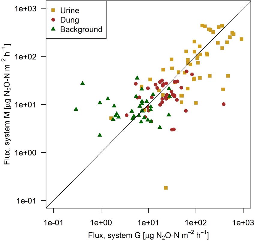
1694                            K. Voglmeier et al.: Grazing-related nitrous oxide emissions: from patch scale to field scale

    1. Background fluxes were parametrized as a function of
       soil moisture at a depth of 5 cm using the soil profile
       information provided in Sect. 2.6 by using a logistic re-
       gression.

    2. Urine patch emissions were parametrized as an expo-
       nential decay function of excreta age. To account for
       different environmental conditions, the deviations of the
       single emissions from this temporal emission pattern
       were again parametrized as a function of soil temper-
       ature and moisture at a depth of 5 cm (Sect. 2.6). Up-
       scaling fluxes to the paddock sizes involved additional
       information on the computed number density of urine         Figure 6. Time series of half-hourly EC flux measurements in both
       patches (as mentioned previously).                          systems during the grazing season 2016. For the analysis of grazing-
                                                                   related emissions, only the non-shaded periods (GOP) were used.
    3. Dung patch emissions were parametrized as a second-         The vertical lines show the timings of fertilization (red) and harvest
       order polynomial function of excreta age. Paddock           (orange) events. Dashed lines indicate that harvest and urea appli-
       emissions were calculated by applying this function to      cation were split for the western (X.11–X.16) and eastern (X.21–
       the computed number of dung patches (as previously          X.25) parts. The shaded areas indicating time periods influenced
       mentioned) per paddock.                                     by fertilization events or harvest were excluded for the evaluation
                                                                   of grazing excreta-related emissions. One flux value (29.0 g N2 O-
The upscaled paddock emissions were finally compared to            N ha−1 h−1 on system M, 30 June 2016) was skipped for better
the EC fluxes by applying the computed footprint fractions         readability.
of the paddocks (Sect. 2.5.4) in order to validate the FB mea-
surements and to quantify the uncertainty of the upscaling
process.                                                           the first full grazing event at the beginning of May were char-
   The area-related N2 O emissions for urine and dung were         acterized by high soil moisture contents (see also Fig. 2a),
also converted to emissions per cow and grazing hour. For          whereas the very wet soil conditions and the corresponding
this purpose, the upscaled paddock emissions were combined         grazing break during June resulted in low fluxes in both sys-
over all paddocks, accumulated for the GOP, multiplied by          tems. The small observed fluxes from the middle of March
the pasture area of each system, and divided by the number         until the end of April resulted mainly from background fluxes
of cows and the grazing duration (Fig. 5). The resulting emis-     and sporadic grazing (Fig. 2c). Occasional negative individ-
sions associated with animal excreta were then related to the      ual flux values between 0 and −1.5 g N2 O-N ha−1 h−1 were
excreted N of the cows (Sect. 2.3) to obtain an excreta-related    observed in both systems (7 %–8 % of the cases). However,
EF that is comparable to the one provided by the IPCC guide-       these fluxes exclusively occurred in cases, when no defined
lines (EF3PRP,CPP ; IPCC, 2006).                                   peak in the cross-covariance function could be identified (and
                                                                   thus the default lag was used, Sect. 2.5.2). Thus it can be
                                                                   concluded that the negative fluxes were generally below the
3     Results                                                      detection limit.
                                                                      During the GOP (excluding the grey shaded fertilizer-
3.1    EC fluxes                                                   influenced time periods in Fig. 6), the fluxes were still very
                                                                   similar for the two pasture systems M and G with a mean
Observed EC fluxes on both pasture systems showed an               and standard deviation of 0.32±0.36 and 0.33±0.37 g N2 O-
almost identical temporal pattern (Fig. 6). The half-hourly        N ha−1 h−1 , respectively. A mean diurnal cycle of the mea-
fluxes on each system showed considerable variation during         sured fluxes could be observed in both systems with the high-
the grazing season with clear peaks after fertilization (grey      est values typically occurring in the afternoon and, on aver-
shaded areas) and after grazing phases in the nearby pad-          age, about 10 %–20 % lower values during the night.
docks (e.g., peaks in May, beginning of August). The overall
highest emissions (29.0 and 24.3 g N2 O-N ha−1 h−1 for sys-        3.2     Chamber fluxes
tems M and G) were measured directly after the fertilizer
application, which followed a harvest of hay at the end of         3.2.1    Comparison of pasture systems
June. This harvest event also led to an increase in the mea-
sured N2 O fluxes (0.5–3.0 g N2 O-N ha−1 h−1 ) which lasted        FB chamber fluxes of background and dung patches were
less than 1 day. The partial fertilizer application in middle of   considerably smaller compared to the fluxes of urine patches
August resulted in higher fluxes compared to the following         (Table 3, Fig. 7). Freshly deposited urine patches under
one in early September. The relatively high emissions during       3 days old could result in N2 O emissions larger than 100

Biogeosciences, 16, 1685–1703, 2019                                                       www.biogeosciences.net/16/1685/2019/
K. Voglmeier et al.: Grazing-related nitrous oxide emissions: from patch scale to field scale 1695
Figure 8. N2 O flux evolution with time for urine patches, dung pats,
and background areas. The fluxes were measured with the fast box
and averaged over 3-day periods, and the error bars show the stan-
dard error of the measurements. The standard errors for the back-
ground fluxes are smaller than the symbols. The dotted lines show
the fitted curves through the averaged values of urine and dung
patch emissions (see also Eqs. 3 and 4).
Figure 7. Scatterplot shows the comparison of near-simultaneous
fluxes for different sources measured with the fast box on the two riods and were related to the excreta age 1tEOG (Fig. 8), de-
pasture systems. The black line indicates the 1 : 1 line. fined as days after EOG (Sect. 2.4.2).
Background fluxes were on average considerably smaller
Table 3. Flux measurements using the FB technique (mean ± SD) than excreta fluxes and showed small persisting emissions
of background and excreta patches averaged over 20 days follow- without systematic dependence on time since grazing. In
ing a grazing phase. Only near-simultaneous measurements in both contrast, for urine patch fluxes a clear relation to 1tEOG was
systems were considered. found. The highest fluxes were usually observed within the
first days after the urination event. Afterwards, they rapidly
Measurement location System M System G decreased with time, although with a high variability that can
partly be attributed to the influence of environmental condi-
Background (µg N2 O-N m−2 h−1 ) 8±8 5±8
Urine (µg N2 O-N m−2 h−1 ) 121 ± 130 162 ± 190
tions (see Sect. 3.2.3). The age-dependent evolution of urine
Dung (µg N2 O-N m−2 h−1 ) 16 ± 18 35 ± 60 patch emissions (FU,age ) was parameterized with an expo-
nential decay function fitted to the data points in Fig. 8:
FU,age = a1 · expb1 ·1tEOG . (3)
times the values of background areas. The relative variability
within the different source classes (urine, dung, background) The coefficients of Eqs. (3)–(8) are presented in Table 4 and
were very high and resulted in standard deviations larger than apply to fluxes in units of µg N2 O-N m−2 h−1 .
the associated mean values. The excreta fluxes measured on Dung patch fluxes also showed a relation to excreta age
system G tended to be somewhat higher in magnitude com- (Fig. 8), however less pronounced compared to urine patches,
pared to system M, but no significant difference (p > 0.05) and the highest emissions were typically observed between 4
was found. Also, for the background fluxes no significant and 11 days after dung deposition. However they were still
(p > 0.05) difference between the two pasture systems was smaller on average than the urine patch emissions during the
observed. Therefore all FB fluxes were combined for further entire observed age period. Because the evolution of dung
processing without taking into account the different pasture emissions FD,age after the observed 20-day age period is un-
systems. clear and a meaningful functional extrapolation was not pos-
sible, we decided to use a simple second-order polynomial
3.2.2 Dependence on excreta age for parameterization purposes. This allowed us to reproduce
the initial increase with age and a rapid decrease to zero be-
The information on the temporal pattern of the excreta and yond the measured age range:
background fluxes after grazing is important for the time in-
tegration of the individual sources and for the comparison FD,age = a2 + b2 · 1tEOG + c2 · 1tEOG 2 . (4)
with the EC measurements. In order to analyze and parame-
terize the temporal evolution of the emissions, the measured The fitted polynomial function is only applicable up to
FB fluxes of each source class were averaged over 3-day pe- 1tEOG ≈ 25 d, where it crosses the zero line.
www.biogeosciences.net/16/1685/2019/ Biogeosciences, 16, 1685–1703, 20191696 K. Voglmeier et al.: Grazing-related nitrous oxide emissions: from patch scale to field scale
Table 4. Coefficients (a–c), corresponding indices i, and signifi-
cance levels for the equations presented in Sect. 3.2. The equation
coefficients were fitted using FB chamber measurements and yield
fluxes in units of µg N2 O-N m−2 h−1 . The input quantities are the
soil temperature TS (in units of degrees Celsius), time since end
of grazing 1tEOG (in units of days), and volumetric water content
VWC (as a dimensionless fraction).
Equation I ai bi ci
Eq. (3) 1 587∗∗∗ −0.082∗∗
Eq. (4) 2 23∗ 5.4∗ −0.25∗
Eq. (5) 3 12.6∗∗∗ 0.267∗∗∗ 0.012∗
Eq. (7) 4 −1490∗∗∗ 2900∗∗∗ 23.9∗∗
Eq. (8) 5 0.098∗∗∗ −0.086∗∗
Figure 9. Surface plot shows the estimated N2 O flux deviation
∗∗∗ Significant at level p < 0.001. ∗∗ Significant at level p < 0.01.
∗ Significant at level p < 0.05.
(Eqs. 6, 7; CorrU,env = 0) from the exponential fit (Eq. 3) for urine
patches depending on soil moisture VWCU and temperature at a
depth of 5 cm. The black dots indicate the conditions under which
flux measurements with the FB were obtained.
3.2.3 Dependence on environmental conditions
Measured chamber fluxes were analyzed in relation to driv- a similar 1tEOG was measured at a low TS (1 ◦ C) and a
ing soil parameters (Sect. 2.6). For dung patch emissions, no lower VWC (0.3). Maximum positive measured FB flux de-
relation to these parameters was found (thus FD = FD,age ). viations (Sect. 2.7) from Eq. (3) were generally observed for
For background fluxes no significant dependence on soil tem- wet (VWC > 0.45) and warm (> 17 ◦ C) soil conditions while
perature (p < 0.05), but a clear dependence on the volumet- low TS and VWC resulted in negative flux deviations. Thus,
ric water content (VWC) at a depth of 5 cm, was found. The the final regression model for urine patch emissions (Eq. 6)
background fluxes had a large variability and could roughly consists of multiple equations (Eqs. 3, 7, 8) which relate the
be separated by three different VWC sectors (< 0.27, 0.27– measured fluxes to the temporal decay (Eq. 3) and a deviation
0.33, > 0.33). In the sector below a VWC of 0.27, fluxes 1FU,env to this decay, where 1FU,env was parametrized as a
typically ranged between −3 and 15 µg N2 O-N m−2 h−1 , function of environmental driving parameters TS and VWCU
whereas in the upper sector above a VWC of 0.33 the fluxes (Eqs. 7 and 8, Fig. 9).
showed typical values between 0 and 30 µg N2 O-N m−2 h−1 .
Nevertheless, the variability was especially pronounced in FU = FU,age + 1FU,env (6)
the VWC range between 0.27 and 0.33 with fluxes ranging 1FU,env = (a4 + b4 · VWCU + c4 · TS )
between 0 and 40 µg N2 O-N m−2 h−1 . Thus this VWC range
· CorrU,env (1tEOG ) (7)
also comprised the overall highest background fluxes. How-
ever, averaging the fluxes by VWC intervals of 0.05 resulted CorrU,env corrects 1FU,env for different urine patch ages as
in very similar values of about 12 ± 3 µg N2 O-N m−2 h−1 the deviation can be larger for relatively new patches com-
above a VWC of 0.3. Hence, the measured background fluxes pared to older ones. This correction factor was found to be
could be parametrized with the following functional relation- a linear relationship (p < 0.01) between 1.35 for a 1tEOG of
ship: 0 days (after the patch deposition) and 0.35 after 20 days.
a3 VWCU (Eq. 8) accounts for different soil moisture condi-
FBG = (b
. (5) tions at the surface below a urine patch and nearby back-
1 + exp 3 −VWC)/c3
ground areas and was parametrized as a function of back-
This logistic regression curve has a strong effect below VWC ground VWC and 1tEOG (Eq. 8).
values of 0.30 but stays fairly constant at higher VWC con-
tents and converges to a flux of 12.6 µg N2 O-N m−2 h−1 . Be- VWCU = VWC + a5 · expb5 ·1tEOG (8)
low a VWC of 0.2 the logistic regression converges to a back-
ground flux of 0 µg N2 O-N m−2 h−1 .
Measured urine patch emissions showed a clear response 3.3 Upscaled chamber fluxes
not only to the excreta age as shown in Sect. 3.2.2 but also to
changes in TS and VWC. On a specific 1tEOG , FU,age could 3.3.1 Comparison between upscaled chamber and EC
vary significantly and typically correlated with soil condi- fluxes
tions. The highest flux (5117 µg N2 O-N m−2 h−1 , 1tEOG =
6 d) was measured at a TS of 18 ◦ C and a VWC of 0.42 Generally the field-scale fluxes represent the area integral
while the lowest measured flux (34 µg N2 O-N m−2 h−1 ) on of management-related (excreta patches) and environmen-
Biogeosciences, 16, 1685–1703, 2019 www.biogeosciences.net/16/1685/2019/K. Voglmeier et al.: Grazing-related nitrous oxide emissions: from patch scale to field scale 1697
Figure 11. Cumulative emissions for both systems obtained with
the FB and EC technique during GOP 2016. The grey shaded
bars indicate time periods which were excluded due to significant
overlapping N2 O emissions from fertilization/harvest and grazing
(Sects. 2.5, 3.1).
Figure 10. Time series of (a) environmental parameters and (b) up-
scaled FB fluxes (Sect. 2.7) for different paddocks (M11–M14) in
system M. The colored rectangles at the bottom show the graz-
ing phases on the four considered paddocks (grey colors indicating in environmental driving parameter could be observed, it was
grazing on the remaining paddocks). (c) N2 O fluxes by EC and up- less pronounced for the upscaled FB fluxes in comparison to
scaled FB during a full rotation between 23 September and 10 Au- the EC fluxes.
gust 2016 for system M. Gap filling of the EC fluxes (Sect. 2.5.3) allowed the cal-
culation of the cumulative N2 O emissions during the GOP
(solid lines in Fig. 11). These area-related emissions were
very similar between the two systems throughout the GOP
tally driven small-scale fluxes. Therefore the relationships with seasonal sums close to 1500 g N2 O-N ha−1 . Cumulating
presented in Sect. 3.2.2 (dependency on excreta age) and the N2 O emissions not only enabled a more quantitative com-
Sect. 3.2.3 (environmental driving parameter) were applied parison between the systems, but also allowed a better com-
to upscale the FB measurements to the paddock size during parison between the two measurement approaches (Fig. 11).
the GOP. The emissions of the upscaled FB matched the EC emis-
As shown as an example in Fig. 10 for an 18-day period, sions rather well with differences of the seasonal sums below
the magnitude of the management-related upscaled paddock 3 %. Distinct differences were mainly observed in May and
fluxes depended mainly on the grazing duration on the single June when FB-derived emissions were significantly overes-
paddocks (similar slope for different paddocks M11–M14). timated compared to EC. At the end of the grazing period
The maximum of the emissions was typically calculated at and averaged over both systems, slightly higher emissions
the end of the grazing period on the respective paddocks. were estimated from the upscaling routine compared to the
The lower limit of the fluxes was given by the estimated measured EC emissions. Monthly absolute differences be-
background fluxes, especially at the beginning of a new ro- tween the cumulative EC and the upscaled cumulative FB
tation, and stayed therefore rather constant for VWC values sums were normally distributed (p < 0.05) with 1σ values
above 0.3 (Eq. 5, Sect. 3.2.3). Variations in environmental of 26 % and 25 % for systems M and G, respectively. Within
conditions (mainly important for soil moisture) led to rapid this uncertainty range no difference between the two mea-
changes in the emission level as long as significant urine surement approaches was observable.
patch emissions were present. These rapid variations typi-
cally occurred after stronger precipitation events (as shown in 3.3.2 Emission breakdown into contribution sources
Fig. 10a for on-site meteorological and soil measurements).
Upscaling the paddock fluxes to the EC footprint allowed The excellent match between the EC fluxes and the upscaled
a direct comparison with the EC fluxes on a half-hourly basis chamber-based fluxes showed that the applied relationships
(Fig. 10c). The upscaled FB fluxes compared well in mag- which used excreta age and environmental parameters as in-
nitude with the measured EC fluxes and showed a similar put (see Sect. 3.2) were reasonable and allowed the separa-
temporal behavior. While generally a response to variations tion into single emission sources (Fig. 12). Except for the be-
www.biogeosciences.net/16/1685/2019/ Biogeosciences, 16, 1685–1703, 2019You can also read