A dynamical systems characterization of atmospheric jet regimes - Earth System Dynamics
←
→
Page content transcription
If your browser does not render page correctly, please read the page content below
Earth Syst. Dynam., 12, 233–251, 2021
https://doi.org/10.5194/esd-12-233-2021
© Author(s) 2021. This work is distributed under
the Creative Commons Attribution 4.0 License.

                         A dynamical systems characterization
                              of atmospheric jet regimes
             Gabriele Messori1,2 , Nili Harnik3 , Erica Madonna4,5 , Orli Lachmy6 , and Davide Faranda7,8,9
                         1 Department   of Earth Sciences and Centre of Natural Hazards and Disaster
                                    Science (CNDS), Uppsala University, Uppsala, Sweden
                 2 Department of Meteorology and Bolin Centre for Climate Research, Stockholm University,

                                                      Stockholm, Sweden
                              3 Department of Geosciences, Tel Aviv University, Tel Aviv, Israel
                                4 Geophysical Institute, University of Bergen, Bergen, Norway
                                   5 Bjerknes Centre for Climate Research, Bergen, Norway
                         6 Department of Natural Sciences, Open University of Israel, Ra’anana, Israel
               7 Laboratoire des Sciences du Climat et de l’Environnement, LSCE/IPSL, CEA-CNRS-UVSQ,

                                         Université Paris-Saclay, Gif-sur-Yvette, France
                                        8 London Mathematical Laboratory, London, UK
                       9 LMD/IPSL, Ecole Normale Superieure, PSL research University, Paris, France

                             Correspondence: Gabriele Messori (gabriele.messori@geo.uu.se)

                                   Received: 26 February 2020 – Discussion started: 6 March 2020
                       Revised: 19 October 2020 – Accepted: 28 December 2020 – Published: 26 February 2021

       Abstract. Atmospheric jet streams are typically separated into primarily “eddy-driven” (or polar-front) jets
       and primarily “thermally driven” (or subtropical) jets. Some regions also display “merged” jets, resulting from
       the (quasi-)collocation of the regions of eddy generation with the subtropical jet. The different locations and
       driving mechanisms of these jets arise from very different underlying mechanisms and result in very different
       jet characteristics. Here, we link the current understanding of dynamical jet maintenance mechanisms, mostly
       arising from conceptual or idealized models, to the phenomena observed in reanalysis data. We specifically
       focus on developing a unitary analysis framework grounded in dynamical systems theory, which may be applied
       to both idealized models and reanalysis, as well as allowing for direct intercomparison. Our results illustrate the
       effectiveness of dynamical systems indicators to diagnose jet regimes.

1   Introduction                                                   theoretical constructs: the former would require an eddy-less,
                                                                   axisymmetric atmosphere (Held and Hou, 1980), while the
                                                                   latter can only exist in the absence of a thermally driven
To zeroth order, the global atmospheric circulation may            meridional advection of zonal-mean angular momentum (e.g.
be construed as arising from the three-way interaction be-         Panetta, 1993). However, there are atmospheric flows that
tween the mean meridional circulation, mid-latitude zonal          approximate these two limiting cases to a good degree, al-
jet streams and baroclinically unstable eddies. Advection of       beit with the caveats discussed below. These are often termed
planetary angular momentum by the mean meridional circu-           “subtropical” and “polar-front” jets in reference to their geo-
lation, specifically by the thermally direct Hadley cell, sup-     graphical locations.
ports so-called “thermally driven” jets (Held and Hou, 1980).         The subtropical jet is an upper-tropospheric jet with a
Convergence of eddy momentum flux by baroclinic eddies             strong vertical shear located at the poleward edge of the
supports so-called “eddy-driven” jets (Held, 1975; Rhines,         Hadley cell. While the observed tropical circulation is dis-
1975). Purely thermally driven or eddy-driven jets are largely

Published by Copernicus Publications on behalf of the European Geosciences Union.
234                                                                    G. Messori et al.: Dynamics of atmospheric jet regimes

tinctly zonally asymmetric (e.g. Heaviside and Czaja, 2013),        to further our understanding of this major component of the
the underlying physical drivers of this flow may be related to      climate system. Our goal in the present study is precisely to
the idealized axisymmetric scenario of Held and Hou (1980).         provide a concise quantitative overview of the jet character-
Poleward of the Hadley cell, the Ferrel cell corresponds to         istics in an idealized atmospheric model and relate them to
a region of strong baroclinic activity. Here, an equivalent         the large-scale flows in the real atmosphere, as reproduced
barotropic polar-front jet exists (e.g. Hoskins et al., 1983).      by reanalysis products. We specifically focus on developing
While the meridional advection of zonal-mean angular mo-            a unitary analysis framework which may be applied to both
mentum in the region is clearly non-zero, we can again relate       the idealized model and reanalysis data, allowing for direct
this jet to one of the idealized limiting cases described above.    intercomparison.
Specifically, two-layer quasi-geostrophic models show that             An idealized model fit for the task at hand should be able
in this region, when a geophysical background flow is per-          to maintain three distinct jet regimes: a thermally driven sub-
turbed, the growing baroclinic waves that result from the per-      tropical jet, an eddy-driven polar-front jet and a merged jet.
turbations can spontaneously generate a jet through converg-        Just as in the real atmosphere, these regimes should differ
ing westerly momentum flux (e.g. Panetta, 1993; Lee, 1997).         in the location and variability of the jet stream, as well as
   The distinction between the subtropical and polar-front          in the structure, zonal wavenumber and phase speed of the
jets is not always evident, and the jets display different char-    dominant modes. Here, we use the two-layer modified quasi-
acteristics depending on geographical location and season.          geostrophic (QG) spherical model of Lachmy and Harnik
In the Northern Hemisphere, the two flows are mostly sep-           (2014). Unlike other QG models, our setup includes advec-
arate during wintertime over the North Atlantic basin, while        tion of the zonal-mean momentum by the ageostrophic mean
over parts of Asia and the Pacific the default atmospheric          meridional circulation. This enables the model to resolve the
configuration is of a single or “merged” jet. This terminol-        momentum balance of the subtropical jet. The model can
ogy is supported by evidence that a single jet results from         therefore reproduce the three different jet regimes and their
the (quasi-)collocation of the regions of eddy generation with      distinct wave-mean flow feedback mechanisms (Lachmy and
the subtropical jet such that the driving mechanisms are both       Harnik, 2016).
thermal and eddy-related (Eichelberger and Hartmann, 2007;             To elucidate the intrinsic dynamical characteristics of the
Li and Wettstein, 2012; O’Rourke and Vallis, 2013; Harnik           different jet regimes, we interpret atmospheric flows as rep-
et al., 2014). In the Southern Hemisphere (SH), the austral         resentative of the evolution of chaotic atmospheric attractors.
summertime circumpolar jet is located around 40–50◦ S, col-         Recent advances in dynamical systems theory have demon-
located with regions of enhanced surface baroclinicity (e.g.        strated that any instantaneous state of a chaotic system may
Nakamura and Shimpo, 2004; Koch et al., 2006). During               be described by two metrics: the local dimension – related
austral winter, a single jet is seen in the Indian Ocean sec-       to the system’s active degrees of freedom around that par-
tor, while two distinct branches emerge in the Pacific sec-         ticular state – and a local measure of persistence (Lucarini
tor: a subtropical jet at around 30◦ S and a polar-front jet        et al., 2016; Faranda et al., 2017b). This approach can easily
at around 60◦ S (e.g. Nakamura and Shimpo, 2004; Gallego            be applied to a variety of datasets, including suitably pro-
et al., 2005; Koch et al., 2006). At upper levels, the strongest    cessed reanalysis data, and may thus be used to provide a
flow is seen for the Pacific subtropical jet, while at lower lev-   direct analogy between modelled and observed flows. Here,
els the flow over the Indian Ocean sector is strongest (e.g.        we apply it for the first time to the study of atmospheric jets
Nakamura and Shimpo, 2004, see also Fig. 1a). While the             in both idealized model and reanalysis data. In doing so, we
climatological picture shows two distinct jets co-existing in       underscore the links that can be made between the dynam-
the Pacific sector, these are not well-separated every year         ical systems metrics and the physical characteristics of the
(Bals-Elsholz et al., 2001; Nakamura and Shimpo, 2004). On          atmospheric flow.
shorter timescales (e.g. days or weeks), we further expect pe-         The connection between the dynamical systems character-
riods when the two jets are merged and others when they are         istics of the flow and the jet regimes arises from the wave
distinct.                                                           spectrum and its interaction with the zonal-mean flow. Ac-
   The different locations and drivers of the two jet struc-        cording to Lachmy and Harnik (2016), the flow in the ideal-
tures, plus the intermediate merged jet, arise from very differ-    ized two-layer modified QG model transitions from a sub-
ent underlying mechanisms. They in turn result in very dif-         tropical jet regime to a merged jet regime and then to an
ferent flow characteristics, for example in terms of the jet’s      eddy-driven jet regime as the eddy energy is increased. At the
variability properties, the wave spectrum and the degree of         transition between the merged and eddy-driven jet regimes,
non-linearity (e.g. Lachmy and Harnik, 2016, 2020). How-            the wave energy spectrum becomes turbulent and an inverse
ever, our understanding of the dynamical maintenance mech-          energy cascade takes place. At this transition, an increase in
anisms mostly relies on conceptual or idealized models (e.g.        the jet’s latitudinal variability and a decrease in its character-
Held and Larichev, 1996; Son and Lee, 2005; Lachmy and              istic variability timescale are also seen (Lachmy and Harnik,
Harnik, 2016; Faranda et al., 2019c). Linking these to the          2020). We expect these changes to be reflected in the dy-
phenomena observed in the real atmosphere is therefore key

Earth Syst. Dynam., 12, 233–251, 2021                                                  https://doi.org/10.5194/esd-12-233-2021
G. Messori et al.: Dynamics of atmospheric jet regimes                                                                          235

namical systems metrics, which capture the active degrees of        and the equilibrated eddy amplitude decreases. We consider
freedom and the persistence of the flow.                            a parameter sweep of 27 different combinations of 7 km
   We first provide a brief overview of the data, model and         ≤ H ≤ 10 km and 0.5 ≤ r ≤ 2. The increments of H and r
analysis approaches in Sect. 2. Sections 3 and 4 outline the        are 0.5 km and 0.5, respectively. We removed the simula-
dynamical characteristics of the different flow regimes in the      tion with H = 8 km and r = 2 from the analysis because it
model and reanalysis, respectively. Finally, we discuss these       was dominated by unrealistically regular oscillations of the
results in the context of both idealized models and studies of      eddy amplitude. These oscillations likely arise from an in-
the observed atmospheric jet, and we draw our conclusions           ternal mode of wave-mean flow interaction, which is much
in Sect. 5.                                                         weaker in the other simulations of the parameter sweep. The
                                                                    numbering of these runs is shown in Table A1. The param-
                                                                    eter values were chosen so that all the observed jet regimes
2     Model, data and analysis tools
                                                                    are captured, while the eddies are not completely stabilized.
2.1    The quasi-geostrophic model
                                                                       In the model, we diagnose jet characteristics using
                                                                    barotropic zonal-mean zonal wind (0.5 × (ul + uu ), where
This study uses the numerical model of Lachmy and Harnik            overbars denote zonal means) and barotropic wave vortic-
(2014), designed as a minimal-complexity representation of          ity (0.5 × (ql + qu )). The two give complementary informa-
jet dynamics. The model is based on the QG approxima-               tion on the flow by considering the zonal mean and the wave
tion for a sphere and includes the interactions between the         fields, respectively. We choose to analyse the barotropic (i.e.
zonal-mean zonal wind, the mean meridional circulation and          vertical mean) variables, since they capture most of the vari-
the eddies, quantified as deviations from zonal-mean values.        ability of both the upper- and lower-layer components. The
To balance the heat and momentum budgets, radiative damp-           analysis was repeated using the 3-D (upper and lower levels)
ing to an equilibrium profile and surface friction are also in-     full potential vorticity and wave potential vorticity fields. The
cluded. The model has two vertical layers, which are meant          results support the conclusions drawn from barotropic zonal-
to represent the lower and upper troposphere. Here, we refer        mean zonal wind and barotropic wave vorticity concerning
to these with the subscripts l and u, respectively. Two key         the relative differences in d and θ between the different jet
aspects of the model are a numerical hyper-diffusion scheme         regimes (not shown).
which dissipates energy away from the smallest scales and
a representation of the advection of zonal-mean momentum            2.2   Reanalysis data
by the mean meridional circulation through an ageostrophic
term. The waves are treated separately from the zonal-mean          Part of the analysis is conducted on data from the European
flow to allow for a clear conceptual separation between them.       Centre for Medium-Range Weather Forecasts ERA-Interim
This modified QG framework allows the study of the com-             reanalysis (Dee et al., 2011). We use daily average winds in-
plex interactions between the mean flow, the waves and the          terpolated at a horizontal resolution of 0.5◦ over the austral
mean meridional circulation while retaining the simplicity of       winters (June, July and August, JJA) of 1979–2017. We focus
an idealized model. Since the QG assumptions are not valid          on a South Pacific domain spanning 120 ◦ W–120◦ E, 15◦ S
close to the Equator, the model dynamics are most relevant to       – 75◦ S (see Fig. 1). This is chosen based on Bals-Elsholz
the extratropics. The crude vertical resolution leads to sharp      et al. (2001), Nakamura and Shimpo (2004), and Koch et al.
regime transitions, which would likely be smoother in a sys-        (2006) to focus on a longitudinal region with coherent jet
tem with higher resolution. Despite its limitations, the model      characteristics displaying a range of jet regimes (see also
nonetheless captures the qualitative characteristics of the ob-     Sect. 4). The jet is diagnosed using the 300 and 850 hPa zonal
served jet regimes (Lachmy and Harnik, 2016). For a detailed        wind. These are widely used isobaric surfaces to study upper-
description of the model equations, we refer the reader to Ap-      and lower-tropospheric flows (e.g. Meleshko et al., 2016),
pendix A.                                                           and we select them here in analogy to the upper- and lower-
   The model setup, radiative equilibrium profile and fixed         level flows in the QG model. The dynamical systems met-
parameter values used here are the same as in Lachmy and            rics (Sect. 2.3 below) are then computed on barotropic zonal
Harnik (2016) and are provided in Appendix A. These are             wind, defined as the average of the zonal wind at these two
meant to mimic wintertime conditions. We focus our analy-           levels. We further calculate eddy kinetic energy (EKE) from
sis, both in the model and in the reanalysis data (Sect. 2.2), on   daily data. To separate the eddy flow field from the mean
the SH because it is closer to zonal symmetry than its north-       component, we apply a 6 d high-pass Lanczos filter with 61
ern counterpart. In the model, the different flow regimes are       weights. The use of EKE allows an effective comparison with
obtained through different combinations of the layer thick-         model results, as this quantity provides a clear separation be-
ness (H ) and the wave-damping (r) parameters. The r pa-            tween model jet regimes (Fig. 2a) and can be used to charac-
rameter specifically represents the ratio between the damp-         terize SH jet variability (e.g. Inatsu and Hoskins, 2004; Sh-
ing parameters for the eddies and for the zonal-mean flow.          iogama et al., 2004).
As H and r are increased, the flow becomes more stable

https://doi.org/10.5194/esd-12-233-2021                                                 Earth Syst. Dynam., 12, 233–251, 2021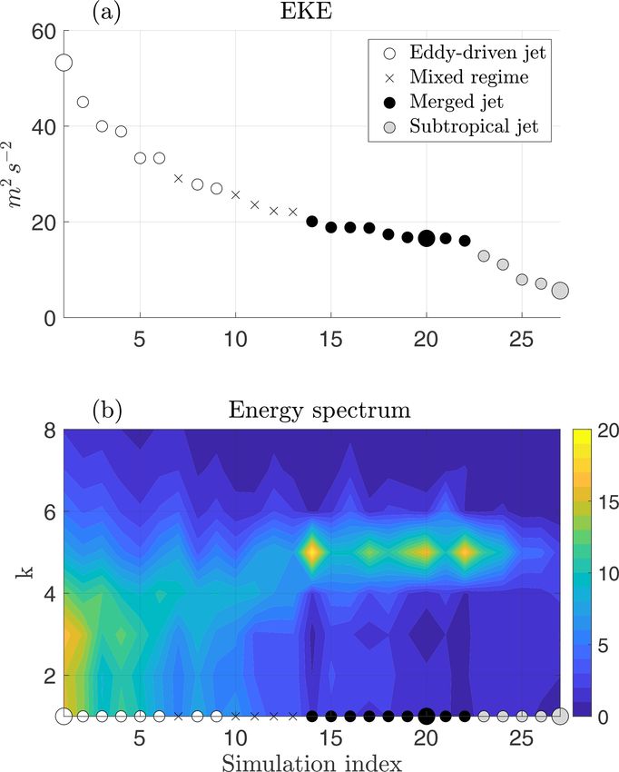
236                                                                        G. Messori et al.: Dynamics of atmospheric jet regimes

Figure 1. Climatological JJA zonal wind (m s−1 , a) and eddy kinetic energy (EKE, m2 s−2 , b). Colours show variables on the 850 hPa
surface and contours on the 300 hPa surface. Contours are at 30 and 40 m s−1 in (a) and every 20 m2 s−2 starting from 60 m2 s−2 in (b). The
red boxes show the South Pacific domain (120 ◦ W–120 ◦ E, 15 ◦ –75 ◦ S).

2.3   Dynamical systems metrics                                         the system persists in states that closely resemble ζ . Both d
                                                                        and θ may be related to a state’s intrinsic predictability (Mes-
The above data are analysed by applying a recently de-                  sori et al., 2017; Hochman et al., 2019). Indeed, the attractor
veloped approach grounded in dynamical systems theory.                  dimension is related to error growth and thus predictability.
This evolved from the findings of Lucarini et al. (2016)                If trajectories are constrained on a low-dimensional mani-
and Faranda et al. (2017b), and it allows computing the in-             fold, they will be more easily predictable than if they evolve
stantaneous (in time) or local (in phase space) properties              on a high-dimensional phase space with many different di-
of a dynamical system by combining extreme value theory                 rections available (Buschow and Friederichs, 2018). This ar-
with Poincaré recurrences. A given succession of latitude–              gument may be extended to d when considering a specific
longitude maps of an atmospheric variable of interest is in-            point on the attractor. Thus, a state with a low d will have
terpreted as a long trajectory in a reduced phase space of the          higher intrinsic predictability than one with a high d. Simi-
atmospheric flow. Each map corresponds to both a specific               larly, one may interpret highly persistent states (high θ −1 ) as
point in this phase space and a specific time. Instantaneous-           having high intrinsic predictability. Indeed, a high θ −1 im-
ness in time is therefore equivalent to locality in phase space.        plies that a persistence forecast – the simplest possible fore-
Local (instantaneous) properties are then computed for all              cast one can make – will roughly capture the short-term evo-
points (time steps) in our dataset. We specifically compute             lution of the state. Forecasting the evolution of highly tran-
two metrics, namely the local dimension d and the persis-               sient states (low θ −1 ) will typically require an understand-
tence θ −1 .                                                            ing of the dynamics of the system and thus correspond to
   The local dimension is the local counterpart to the attrac-          lower intrinsic predictability. However, since the degree of
tor dimension of a dynamical system, the attractor being a              predictability is jointly determined by d and θ , specific dy-
geometrical object defined in the phase space hosting all the           namical regimes such as travelling linear waves may be com-
possible states of the system. The local dimension describes            paratively predictable and display a low d yet also a low per-
the geometry of the system’s trajectory in a small region of            sistence. The fact that both d and θ −1 are local metrics im-
the phase space around a state of interest ζ , which in our case        plies that the intrinsic predictability is conceptually different
could be a latitude–longitude map of barotropic zonal wind              from the predictability inferred from the performance of a
from reanalysis data; d may specifically be taken as a proxy            numerical weather prediction model. Although the informa-
for the number of active degrees of freedom of the system               tion provided by the two partly overlaps (Scher and Messori,
about ζ . In other words, it measures how many directions all           2018), the former depends on the local geometry of the at-
possible trajectories originating from a certain state in phase         tractor and on the characteristic timescales of the dynamics
space can locally take on the attractor. The persistence θ −1 of        in the neighbourhood of the state of interest. On the other
a state ζ is a measure of the system’s typical residence time           hand, the numerical forecasts depend on the specific numer-
in the neighbourhood of ζ : that is, a measure of how long

Earth Syst. Dynam., 12, 233–251, 2021                                                       https://doi.org/10.5194/esd-12-233-2021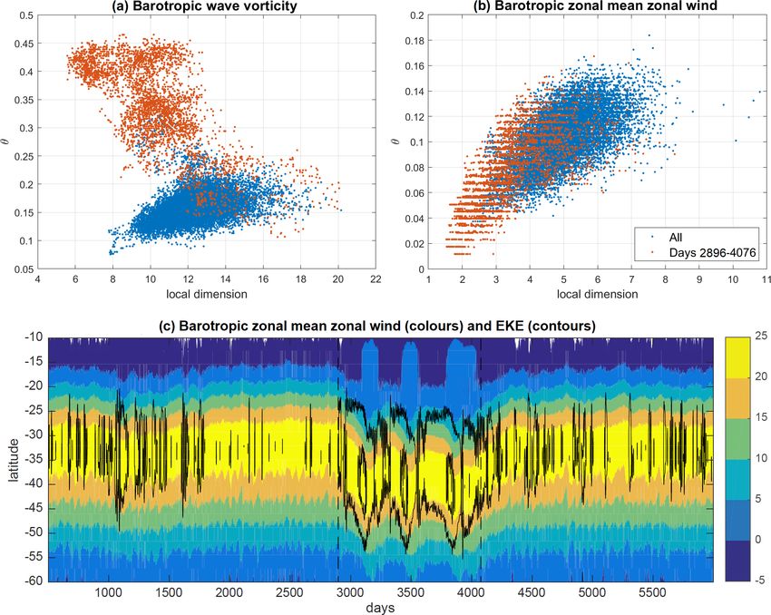
G. Messori et al.: Dynamics of atmospheric jet regimes                                                                            237

                                                                        dataset whose time step is smaller than the typical timescale
                                                                        of the physical processes of interest. An overly long time
                                                                        step would indeed result in all instantaneous states tending
                                                                        to θ −1 = 1. In line with previous studies, we deem daily data
                                                                        sufficient to capture the salient features of the large-scale
                                                                        jet variability (e.g. Woollings et al., 2010; Madonna et al.,
                                                                        2017).
                                                                           As a final product of our analysis, one obtains a value of
                                                                        d and θ −1 for every time step and variable in the dataset.
                                                                        Estimating d and θ −1 for real-world data is subject to a
                                                                        number of caveats, as discussed in Appendix B. There are
                                                                        nonetheless both formal and empirical arguments supporting
                                                                        the application of our framework to data that deviate from
                                                                        the theoretical case, and indeed the two dynamical systems
                                                                        metrics have been successfully applied to a variety of cli-
                                                                        mate datasets (e.g. Rodrigues et al., 2018; Scher and Mes-
                                                                        sori, 2019; Hochman et al., 2020; Faranda et al., 2019a, b;
                                                                        Brunetti et al., 2019; De Luca et al., 2020a, b) and more gen-
                                                                        erally to a range of chaotic dynamical systems (Faranda et al.,
                                                                        2020; Pons et al., 2020).

                                                                        3     Dynamical characteristics of jet regimes in a
                                                                              two-layer QG model

                                                                        3.1    Model jet regimes
Figure 2. (a) Time-mean eddy kinetic energy (EKE) averaged over
the model’s Southern Hemisphere and (b) the eddy energy spec-
                                                                        The simple model we adopt can reproduce the three jet
trum as a function of zonal wavenumber k and simulation index           regimes: subtropical, merged and eddy-driven. We classify
(see Table A1). Units are m2 s−2 for both panels. The markers in        our simulations according to the structure and driving mecha-
both panels indicate the jet regime of each simulation. Open circles,   nism of the zonal-mean zonal wind and according to the vari-
black circles, grey circles, and × indicate the different jet regimes   ability and spectral properties of the flow, following Lachmy
as in the legend. The larger markers indicate the simulations shown     and Harnik (2016). The subtropical jet is located at the edge
in Fig. A1.                                                             of the Hadley cell, displays weak eddy kinetic energy and
                                                                        is maintained by zonal-mean advection of planetary momen-
                                                                        tum. The merged jet is located inside the Ferrel cell and is
ical model used and, for forecasts with a long lead time, on            maintained mainly by eddy momentum flux convergence. It
non-local properties of the trajectory.                                 has a narrow latitudinal structure and a very low latitudinal
   To estimate the local dimension we leverage the Freitas–             variability. The eddy-driven jet is also maintained by eddy
Freitas–Todd theorem (Freitas et al., 2010), modified by Lu-            momentum flux convergence, but it is much wider than the
carini et al. (2012), which characterizes the system’s recur-           merged jet and displays large fluctuations between a single-
rences around the state of interest ζ . The theorem specifically        and double-jet structure. The characterization of the different
indicates that the cumulative distribution function of suitably         flow regimes is further detailed in Appendix A. As the wave
defined recurrences of the system about ζ converges to the              energy is increased by decreasing H and/or r (Sect. 2.1), the
exponential member of the generalized Pareto distribution               flow transitions from a subtropical jet regime to a merged jet
(GPD). As detailed in Appendix B, the local dimension may               regime and finally to an eddy-driven jet regime. In Fig. 2a,
then be estimated directly from the parameters of the GPD.              the different simulations are marked according to the flow
Here, we follow the estimation procedure of Faranda et al.              regime and sorted by their time-mean EKE. The different
(2019b).                                                                spectral properties of the flow in the three regimes are ap-
   The persistence is instead obtained from the extremal in-            parent in Fig. 2b. In the merged jet regime the wave spec-
dex, which we can interpret as the inverse of the mean clus-            trum is dominated by a wavenumber 5 mode, whereas in the
ter size of recurrences about ζ (Moloney et al., 2019). Further         eddy-driven jet regime the spectrum is much wider and ex-
details on the estimation of the extremal index and the deriva-         tends to lower wavenumbers. The model further reproduces
tion of θ are provided in Süveges (2007) and Appendix B                 flows which are a mixture of the eddy-driven and merged
here. The persistence is bounded in [1, ∞] and is in units              jet regimes, meaning that the simulations either vacillate be-
of the time step of the data. It is therefore essential to use a        tween the two regimes or that the flow displays character-

https://doi.org/10.5194/esd-12-233-2021                                                    Earth Syst. Dynam., 12, 233–251, 2021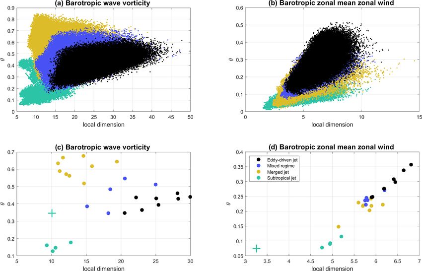
238                                                                  G. Messori et al.: Dynamics of atmospheric jet regimes

istics of both regimes, depending on the chosen diagnostic        plays a low persistence due to its relatively fast phase prop-
variable (crosses in Fig. 2).                                     agation. Consistently, the quasi-linear nature of this regime,
                                                                  in which the waves weaken the jet in place while they de-
3.2   Dynamical characteristics of the model jet regimes
                                                                  cay, results in d and θ values of the barotropic zonal-mean
                                                                  zonal wind which lie between those of the linear subtropical
The differences in the time-mean EKE and EKE spectra of           jet regime and the turbulent eddy-driven jet regime (Fig. 3b,
the three jet regimes (plus the mixed case) reproduced by the     d).
model are related to their different spatio-temporal variabili-      A more detailed picture of the evolution of the flow’s dy-
ties (see also Sect. 3.1 and Lachmy and Harnik, 2020). This,      namical characteristics can be obtained by ranking the dif-
in turn, suggests that their dynamical systems characteristics    ferent simulations by decreasing EKE, which closely mir-
should be different. Wave driving is the dominant mecha-          rors the division between the different jet regimes (Fig. 4).
nism affecting the jet and its variability on a wide range of     The barotropic wave vorticity displays an increase in θ at the
timescales. A strong EKE and a wide EKE spectrum should           transition between the eddy-driven and merged jet regimes,
favour non-linearities in the flow and allow for a rich set of    as well as a large discontinuous decrease in θ at the transi-
possible evolutions. The converse holds for weak EKE and a        tion between the merged and subtropical jet regimes around
narrow EKE spectrum. We would thus expect the jet stream          simulation 23 (Fig. 4a). The latter simulation is discussed
to be more persistent (smaller θ ) and display a lower local      in further detail below. As discussed above, we interpret the
dimension d when the EKE is weak and the spectrum is nar-         large values of θ in the merged jet regime, which indicate
rower (see also Sect. 5).                                         low persistence, as a result of the regime’s narrow spec-
   We analyse the results for d and θ computed on both            trum with a single dominant propagating wave mode. The
barotropic zonal-mean zonal wind and barotropic wave vor-         barotropic wave vorticity d, on the other hand, shows a de-
ticity (Fig. 3). The former (Fig. 3b, d) displays increasing d    crease as a function of EKE, albeit with significant variability
and θ as the flow transitions from the weak EKE subtropical       within the individual jet regimes. The highest values of d ap-
jet regime (turquoise dots) to the mid-range EKE merged jet       pear in the most energetic simulations of the eddy-driven jet
(amber dots) and to the strong EKE eddy-driven jet regime         regime, consistent with their turbulent nature as seen in the
(black dots) via the mixed cases (blue dots). Although the        wave spectrum (Fig. 2b) and also discussed in Lachmy and
spread in d and θ within each simulation is large, the cen-       Harnik (2016). Both dynamical metrics for the barotropic
troids of the different simulations are organized in specific     zonal-mean zonal wind (Fig. 4b, d) display a largely mono-
regions in the d–θ phase space according to the correspond-       tonic decrease with increasing simulation index. Again, the
ing jet regime (Fig. 3d).                                         transitions between different jet regimes, especially that be-
   The picture from the barotropic wave vorticity is more         tween the merged and subtropical jet regimes (around sim-
nuanced (Fig. 3a, c). The subtropical jet regime (turquoise       ulation 23), emerge as discontinuities. Figure 4 also high-
dots) typically displays low d and θ , matching the expected      lights the range of variability of the dynamical systems met-
weak wave activity and the dominance of thermal mainte-           rics within each simulation. Some distributions, such as the
nance mechanisms. The eddy-driven jet regime (black dots)         local dimension of the subtropical jet regime computed on
shows higher d and θ , reflecting the dominant role of ed-        barotropic wave vorticity (Fig. 4c), are very peaked, indicat-
dies and the large meridional excursions in jet location. The     ing homogeneous characteristics of the flow throughout the
merged jet regime (amber dots) and mixed cases (blue dots)        simulations. Others, such as the eddy-driven regime in the
display on average a lower d yet a higher θ than the eddy-        same panel, display a broader peak and a wider range of vari-
driven jet regime, although the mixed and eddy-driven cases       ability, pointing to the rich dynamical structure of the flow.
show substantial overlap in both indicators. A low local di-         We conclude the overview of the QG model’s jet regimes
mension coupled with a low persistence is a somewhat un-          by focusing on simulation no. 23, which serves well to illus-
usual combination in terms of both our a priori expectations      trate the sensitivity of the dynamical systems metrics to the
for the dynamical characteristics of the different jet regimes    instantaneous characteristics of the atmospheric flow. This
and the positive correlation between d and θ displayed by         simulation falls within the subtropical jet regime (Table A1
most atmospheric variables (e.g. Faranda et al., 2017a, b;        and Fig. 2a) but displays some anomalous characteristics dur-
Messori et al., 2017). This result may reflect the narrow wave    ing a period of approximately 1200 d in the middle of the
spectrum driving the merged jet regime, leading to a quasi-       simulation (Fig. 5c). These are clearly visible in Fig. 4 but
periodic behaviour in which wave trains with a dominant           also emerge in Fig. 3a as a cloud of turquoise points extend-
zonal wavenumber develop and circle the globe with a rel-         ing towards high θ values. During this period, the flow is
atively high phase speed (due to the relatively strong jet) be-   characterized by vacillations between a high-EKE, southerly
fore decaying. The wave field evolution is thus a highly pre-     merged jet regime and a subtropical jet. Unlike the mixed jet
dictable eastward translation with low wind speed variability     simulations, however, this is an isolated occurrence, explain-
and a weak meridional meandering of the jet, as reflected in      ing why the simulation falls into the subtropical jet classifi-
the low local dimension. At the same time, the wave field dis-    cation. The dynamical systems metrics enable us to clearly

Earth Syst. Dynam., 12, 233–251, 2021                                                https://doi.org/10.5194/esd-12-233-2021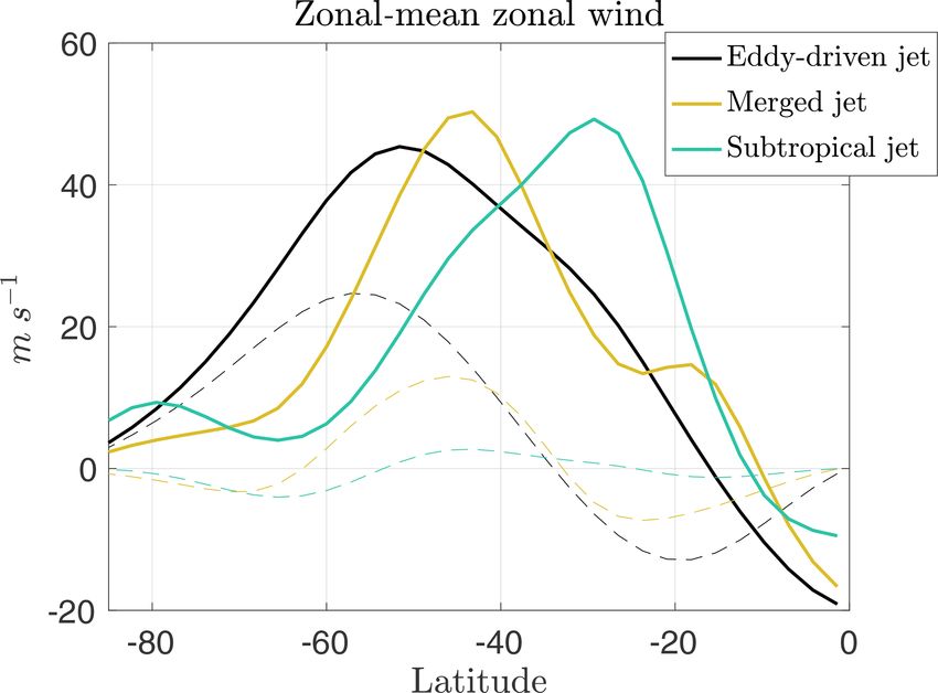
G. Messori et al.: Dynamics of atmospheric jet regimes                                                                                      239

Figure 3. d–θ diagrams of barotropic wave vorticity (a, c) and barotropic zonal-mean zonal wind (b, d) for all time steps in the model
simulations (a, b) as well as centroids for each different simulation. Colours indicate the different jet regimes as in the legend. The turquoise
+ symbols in (c, d) mark the centroids of the anomalous period in simulation no. 23, which is discussed in Sect. 3.2. Note that higher (lower)
θ values correspond to lower (higher) persistence and that the axis ranges differ across the panels.

identify this anomalous transition period (red dots in Fig. 5a,            characteristics (e.g. Bals-Elsholz et al., 2001; Nakamura and
b), which covers a separate region of the d–θ space com-                   Shimpo, 2004; Woollings et al., 2010; Harnik et al., 2014;
pared to the rest of the simulation. Indeed, the outcropping               Messori and Caballero, 2015; Madonna et al., 2017). On this
region in Fig. 3a can be almost exclusively ascribed to the                basis, we expect the jets observed in the real atmosphere
anomalous period (compare Figs. 3a and 5a). The persis-                    to blend the dynamical characteristics of the different jet
tence of this period for the barotropic wave vorticity is inter-           regimes reproduced in the QG model.
mediate between the merged jet and subtropical jet clusters,                  To verify whether our dynamical systems approach can
while the local dimension is close to that of the subtropical              distinguish between different jet regimes in the real atmo-
jet cluster (turquoise cross in Fig. 3c). The barotropic zonal-            sphere, we therefore take a slightly different angle from
mean zonal wind instead displays anomalously low local di-                 that used in our idealized model, although the analysis tools
mension and persistence, with the former being much lower                  are identical to those used above. We compute d and θ
than even those of the linear subtropical jet regime (turquoise            on barotropic zonal wind (see Sect. 2.2) but consider flow
cross in Fig. 3d). Thus, in simulation no. 23 the dynamical                anomalies associated with concurrent low or high values of
systems metrics reflect the transition of the jet to a state with          d and θ . We define these as values beyond the 10th or 90th
peculiar dynamical properties.                                             percentiles of the respective distributions. The choice of joint
                                                                           high or low percentiles is dictated by the fact that the differ-
                                                                           ent jet regimes in Fig. 3b and d align chiefly along a d–θ
4   Dynamical characteristics of jet regimes in                            diagonal. The analysis focuses on austral winter (JJA) over
    reanalysis data                                                        the Pacific domain shown in Fig. 1, which is chosen because
                                                                           it displays a variety of jet regimes. During the austral winter,
As discussed in the Introduction, purely thermally driven                  the signature of the subtropical – and predominantly ther-
or eddy-driven jets are largely theoretical constructs. More-              mally driven – jet is evident at upper levels around 30◦ S,
over, for a given region and season, the jet typically displays            while that of the polar – and predominantly eddy-driven – jet
large intraseasonal variability and a range of different flow              emerges most clearly at lower levels around 60◦ S (Fig. 1).

https://doi.org/10.5194/esd-12-233-2021                                                         Earth Syst. Dynam., 12, 233–251, 2021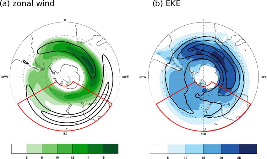
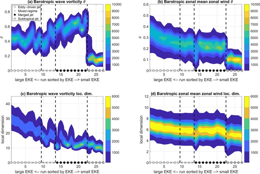
240                                                                            G. Messori et al.: Dynamics of atmospheric jet regimes

Figure 4. Distributions of θ (a, b) and d (c, d) values for barotropic wave vorticity (a, c) and barotropic zonal-mean zonal wind (b, d) in the
different model runs. The colour scale starts at 100 data points and indicates the number of data points per bin. Bin intervals are 0.05 (θ) or 1
(d). The markers on the x axis indicate the flow regime, as in Fig. 2. The vertical dashed lines indicate the approximate transitions between
the different jet regimes. Note that higher (lower) θ values correspond to lower (higher) persistence and that the ordinate ranges differ across
panels.

Periods when these flows are well-separated alternate with                 climatology jet around 30 ◦ S and an anomalous secondary
periods dominated by a single nearly barotropic flow, akin to              maximum at around 55◦ S, associated with large positive
a merged jet.                                                              zonal wind speed anomalies (Fig. 6b). At low levels, there is
   When both d and θ are anomalously low, the upper-                       a single jet located just to the north of 60 ◦ S associated with
level zonal wind (300 hPa) displays a clear maximum around                 large positive zonal flow anomalies (Fig. 6d). The southern
30◦ S, coincident with the climatological location of the                  jet therefore has a more pronounced barotropic structure than
subtropical jet and characterized by above-average speeds                  its northern counterpart, as also seen in the vertical cross sec-
(Fig. 6a). The signature of this jet extends to the lower tro-             tion of the zonal flow (Fig. 6f). The EKE anomalies are pre-
posphere, where a low-level (850 hPa) zonal wind maximum                   dominantly positive across the central and southern portions
located slightly poleward of the 300 hPa maximum is clearly                of the domain (Fig. 7b, d). The above points to a primarily
visible on the same days, especially in the eastern part of the            eddy-driven jet in the south and a primarily thermally driven
domain (Fig. 6c). This inference is confirmed by analysing                 jet further north, in agreement with the theoretical framework
the vertical cross section of the zonal flow, which evidences              of Lee and Kim (2003) and Son and Lee (2005). It also sug-
a poleward displacement of the location of the zonal wind                  gests that the persistence of the double-jet configuration, with
maximum at 850 hPa compared to 300 hPa (Fig. 6e). The                      a strong eddy-driven jet, is lower (high θ ) than that of the sin-
EKE shows widespread negative anomalies across the cen-                    gle merged jet (low θ ).
tral and southern portions of the domain and localized pos-
itive anomalies at 300 hPa matching the latitude of the jet                5   Discussion and conclusions
(Fig. 7a, c). We interpret the above characteristics as the sig-
nature of a merged jet.                                                    We have analysed different jet regimes in a set of ideal-
   When both d and θ are anomalously high, the upper-                      ized simulations with a QG model and reanalysis data. The
level zonal flow evidences two maxima: a weaker-than-                      QG model reproduces the full range of theoretically derived

Earth Syst. Dynam., 12, 233–251, 2021                                                           https://doi.org/10.5194/esd-12-233-2021
G. Messori et al.: Dynamics of atmospheric jet regimes                                                                                  241

Figure 5. The d–θ diagrams of barotropic wave vorticity (a) and barotropic zonal-mean zonal wind (b) for all time steps in simulation no. 23
(see Table A1). (c) Latitude–time diagram of barotropic zonal-mean zonal wind (m s−1 , colours) and eddy kinetic energy (EKE, m2 s−2 ,
contours) for the same simulation. The red dots in (a, b) correspond to days 2896–4076 in the simulation. These were chosen based on a
visual inspection of panel (c) and are marked by the two vertical dashed lines. Contours in (c) are at 60 and 120 m2 s−2 . Note that the axis
ranges differ between panels (a) and (b).

jet regimes (e.g. Lee and Kim, 2003; Son and Lee, 2005;                  model and those seen in the ERA-Interim dataset. Such an
Lachmy and Harnik, 2016). These are an eddy-driven jet,                  approach is grounded in dynamical systems theory and is
a merged jet and a subtropical jet. It additionally repro-               based on two metrics, d and θ, which characterize the in-
duces transition states between a merged and eddy-driven                 stantaneous (local in phase space) dynamical characteristics
jet, which we term mixed jets. Pure eddy-driven or thermally             of the jet. The local dimension d is a proxy for the num-
driven jets are largely theoretical constructs, and in the real          ber of active degrees of freedom of the system. The persis-
atmosphere the separation between them is often blurred.                 tence θ −1 is a measure of the typical residence time of the
Nonetheless, it is possible to identify primarily eddy-driven,           system in the neighbourhood of a given state. Their compu-
primarily thermally driven and merged jets (e.g. Koch et al.,            tation arises from an analysis of recurrences of the system,
2006; Eichelberger and Hartmann, 2007; Li and Wettstein,                 and both may be related to the concept of predictability. In-
2012). The South Pacific sector is of particular interest in             deed, one may expect low d, high θ −1 states to be more pre-
this context, since it is a region where the three main jet              dictable than high d, low θ −1 situations (see Sect. 2.3). This
regimes may be observed at the same longitude (e.g. Bals-                interpretation is confirmed by ongoing work by some of the
Elsholz et al., 2001; Nakamura and Shimpo, 2004).                        authors, which finds a direct link between precipitation fore-
   Relating the different jet regimes identified in idealized            cast skills at single stations in France and the values of d
models to those identified in reanalysis data is far from im-            and θ computed for 500 hPa geopotential height fields in the
mediate. Here, we have proposed an analysis approach which               preceding days. Unlike conventional approaches which diag-
may be applied to both datasets and which provides a di-                 nose the driving mechanisms of the jet in terms of complex
rect link between the characteristics of the jets in the QG              physical processes, such as convection or eddy momentum

https://doi.org/10.5194/esd-12-233-2021                                                       Earth Syst. Dynam., 12, 233–251, 2021
242                                                                          G. Messori et al.: Dynamics of atmospheric jet regimes

Figure 6. JJA zonal wind composites (m s−1 ) at 300 hPa (a, b) and 850 hPa (c, d) as well as zonal-mean zonal wind composite cross sections
over the South Pacific domain (120 ◦ W–120 ◦ E). Separate composites are shown for days displaying low (a, c, e) and high (b, d, f) values
of d and θ . See text for details. In (a)–(d), colours show deviations from the climatology, while contours show absolute values. Contours are
every 10 m s−1 starting from 30 m s−1 in (a) (b) and every 3 m s−1 starting from 6 m s−1 in (c, d).

flux convergence, the dynamical systems metrics allow us to              of hours – and versatile in terms of applicability to very dif-
delineate the dynamical properties of the jet uniquely from              ferent datasets (see Rodrigues et al., 2018; Faranda et al.,
computing d and θ on the wind itself. Differently from previ-            2019c; Pons et al., 2020). Moreover, d and θ do not require
ous studies using this approach, here we have thus attempted             prior knowledge of the exact location of the jet.
to link the dynamical systems metrics directly to the physical              In the QG model, d and θ allow us to characterize
mechanisms of jet maintenance. As a caveat, we note that the             the different jet regimes. Specifically, when computed on
absolute values of these metrics should be interpreted in a rel-         barotropic zonal-mean zonal wind they highlight the eddy-
ative sense within each dataset they are computed on and that            driven jet as being a low-persistence, high-dimensional
direct comparison of their magnitudes across datasets should             regime, the subtropical jet as being a high-persistence, low-
be treated with caution. From a theoretical standpoint, there            dimensional regime and the merged jet as having interme-
are cogent arguments supporting the use of recurrences of ob-            diate dynamical characteristics. This reflects the wide wave
servables of a system to investigate the properties of the sys-          spectrum and large latitudinal fluctuations in the eddy-driven
tem’s underlying phase space, even though all the variables              jet versus the lower latitudinal variability of the subtropical
defining said phase space cannot be considered (e.g. Faranda             jet. Indeed, in the former regime the energetic wave activ-
et al., 2017a, c; Barros et al., 2019). This makes our analysis          ity, the comparatively broad wave spectrum and the range
affordable in terms of computational and data requirements –             of wave phase speeds offer a variety of different temporal
indeed, d and θ for a single variable from a reanalysis dataset          evolutions of the atmospheric flow. In the latter regime, the
may be computed by a modern laptop computer in a matter                  flow instead displays a weak eddy kinetic energy and a nar-

Earth Syst. Dynam., 12, 233–251, 2021                                                         https://doi.org/10.5194/esd-12-233-2021
G. Messori et al.: Dynamics of atmospheric jet regimes                                                                               243

Figure 7. JJA EKE composites (m2 s−2 ) at 300 hPa (a, b) and 850 hPa (c, d) for days displaying low (a, c) and high (b, d) values of d and
θ . See text for details. Colours show deviations from the climatology, while contours show absolute values. Contours are every 20 m2 s−2
starting from 40 m2 s−2 in (a, b) and every 5 m2 s−2 starting from 10 m2 s−2 in (c, d).

row wave spectrum, with a correspondingly narrow range of              d and θ time steps, the jet also displays a much sharper EKE
wave phase speeds and meridional excursions. Moreover, the             spectrum (not shown) and a more equatorward lower-level
typically similar wavelength and phase speed of the waves              jet (red line, Fig. A2d) than climatology. On the other hand,
implies that the temporal evolution of the atmospheric flow            when d and θ are anomalously large, the lower-level jet is
is relatively repetitive. Lachmy and Harnik (2016, 2020) fur-          slightly more poleward and intense than usual (compare the
ther analysed the EKE budgets of different jet regimes in              grey and blue lines in Fig. A2d), and the spread in jet profiles
terms of the contributions by linear versus eddy–eddy inter-           is unusually low (blue line in Fig. A2c). The resemblance be-
actions and found that the degree of linearity of the dynamics         tween low d and θ time steps in an eddy-driven jet simulation
changes. The subtropical regime is comparatively linear, the           and the flow characteristics seen in merged jet regime simu-
merged regime’s variability is dominated by wave-mean flow             lations is consistent with inter-regime differences in the two
interactions, and the eddy-driven regime is non-linear with a          dynamical systems indicators. Indeed, simulations classified
turbulent upscale energy cascade. Intuitively, we expect the           as merged jet regimes generally display lower d and θ val-
predictability of the flow to decrease and the jet structure to        ues than simulations within the eddy-driven regime (Fig. 3b).
vary more strongly in time as the flow becomes more non-               Lachmy and Harnik (2020) also found that the temporal vari-
linear. The dynamical systems metrics thus reflect the theo-           ability of the eddy-driven jet includes a merged-jet-like state.
retical expectations of the role of increased EKE in decreas-             The results for reanalysis data largely mirror those found
ing predictability (Leith, 1971). In contrast to the jet vari-         for the idealized simulations. Focusing on the Pacific sector
ability, the model’s jet speed (Fig. A1) is not related to the         of the Southern Ocean, d and θ computed on the barotropic
degree of non-linearity of the flow. Because of this, changes          zonal wind again discriminate between different jet regimes.
in jet speed may not map directly onto differences in d and            Specifically, high d, high θ days display both a thermally
θ.                                                                     driven subtropical jet and a strong eddy-driven polar-front
   A natural question to ask is whether d and θ also re-               jet, while low d, low θ days display a merged jet. A key dif-
flect variability within the individual simulations in the QG          ference from the results in the QG model is that, in the re-
model. A preliminary analysis of the barotropic zonal-mean             analysis data, the South Pacific sector we consider does not
zonal wind for one of the simulations classified as an eddy-           display a purely thermally driven nor a purely eddy-driven
driven regime (simulation no. 2; see Table A1) shows that,             jet. Indeed, both jet regimes co-occur at different latitudes
when d and θ are very low, the jet has large variability (red          during winter. The upper-level jet is stronger in the single-jet
line in Fig. A2c) and a narrow profile reminiscent of the              merged configuration compared to the double-jet configura-
merged jet regime (compare the red line in Fig. A2b with the           tion (compare Fig. 6a and b), consistent with the idealized
amber line in Fig. A1). This may be contrasted with the aver-          results of Son and Lee (2005).
age jet structure for this simulation, which is quite wide with
an inflection suggestive of a separation between the eddy-
driven and subtropical jets (grey line, Fig. A2b). During low

https://doi.org/10.5194/esd-12-233-2021                                                     Earth Syst. Dynam., 12, 233–251, 2021
244                                                               G. Messori et al.: Dynamics of atmospheric jet regimes

   The distinction between eddy-driven, merged and subtrop-
ical jets also applies to the Northern Hemisphere (NH) (e.g.
Eichelberger and Hartmann, 2007; Li and Wettstein, 2012).
Moreover, within the same ocean basin the jet can transi-
tion between different regimes. Therefore, there is no a priori
reason that our analysis framework should not be applicable
to NH dynamics. For example, in the North Atlantic sector
one may expect the climatological co-existence of an eddy-
driven jet and a subtropical jet to correspond to high d and θ
states and the rarer merged jet conditions (e.g. Harnik et al.,
2014; Madonna et al., 2019) to correspond to lower d and θ
values. However, zonal asymmetries linked to land–sea con-
trast and orography are more prominent than in the SH (e.g.
Brayshaw et al., 2009). The observed separation in d–θ space
between the different jet regimes may be affected by this, al-
though it is not straightforward to infer exactly how without
conducting a full analysis. Here, our intention is not to pro-
vide a systematic analysis of atmospheric jet characteristics
in different geographical regions. Rather, by building upon
both idealized simulations and reanalysis data, we illustrate
the potential of dynamical systems indicators to diagnose jet
regimes in a conceptually intuitive fashion.

Earth Syst. Dynam., 12, 233–251, 2021                                           https://doi.org/10.5194/esd-12-233-2021
G. Messori et al.: Dynamics of atmospheric jet regimes 245
Appendix A: Description of the two-layer QG model Table A1. The model simulations sorted by the EKE in descending
order. The parameters H and r are the layer thickness in kilome-
The two-layer QG model, described in Sect. 2.1, solves the tres and the dimensionless wave-damping parameter, respectively.
The simulations are categorized according to their flow regime (see
equations outlined below for the barotropic (vertical mean)
text). Simulations with mixed properties of the merged jet and eddy-
and baroclinic (half the difference between the upper and
driven jet regimes are denoted as a “mixed regime”.
lower layers) components of the zonal-mean zonal momen-
tum equation,
Simulation index H r Flow regime
1 7 0.5 Eddy-driven jet
∂ U 0V 0
∂U M 1 ∂ 1 2 7.5 0.5 Eddy-driven jet
M
=− U T (Va )T − 3 7 1 Eddy-driven jet
∂t a ∂µ a ∂µ 4 8 0.5 Eddy-driven jet
UM − UT ∂ 4U M 5 8.5 0.5 Eddy-driven jet
− −ν , (A1a) 6 7.5 1 Eddy-driven jet
2τf ∂µ4
7 7 1.5 Mixed regime
!
∂ U 0V 0 8 9 0.5 Eddy-driven jet
∂U T 1 ∂U M 1 T
= 2µ − (Va )T − 9 8 1 Eddy-driven jet
∂t a ∂µ a ∂µ 10 9.5 0.5 Mixed regime
11 10 0.5 Mixed regime
UM − UT ∂ 4U T
+ −ν , (A1b) 12 7.5 1.5 Mixed regime
2τf ∂µ4 13 8.5 1 Mixed regime
14 10 1 Merged jet
15 9 1 Merged jet
and the diagnostic equation for (Va )T ,
16 7 2 Merged jet
! 17 9.5 1 Merged jet
2 1 − µ2 ∂ 2 (Va )T 18 8 1.5 Merged jet
µ ∂U M
− + 2µ2 − (Va )T 19 8.5 1.5 Merged jet
∂µ2 a ∂µ 20 9 1.5 Merged jet
21 7.5 2 Merged jet
2
2 ∂ U 0V 0
1−µ ∂
0 ψ0 + µ
T 22 8.5 2 Merged jet
= µVM T
a 2 ∂µ2 a ∂µ 23 9.5 1.5 Subtropical jet
µ µ 24 9 2 Subtropical jet
− UM − UT + (UT )E − U T , (A2) 25 10 1.5 Subtropical jet
2τf τr
26 9.5 2 Subtropical jet
27 10 2 Subtropical jet
where U ≡ u · cos φ, V ≡ v · cos φ and µ ≡ sin φ. The vari-
ables u and v are the zonal and meridional winds, respec-
tively, and φ is the latitude. Subscripts M and T denote the ∂qT0 UM ∂q 0 UT ∂q 0 V 0 ∂q T
=− T − M − M
barotropic and baroclinic components, respectively. Over- ∂t a 1 − µ2 ∂λ a 1 − µ2 ∂λ a ∂µ
bars denote zonal means and primes denote deviations from !0 !0
V 0 ∂q M UM0 ∂q 0 UT0 ∂q 0
the zonal mean. The constants , a, τf , τr and ν are the − T − T − M
a ∂µ a 1 − µ2 ∂λ a 1 − µ2 ∂λ
Earth’s rotation rate and radius, the surface friction timescale,
VM ∂qT0 0 0
∇ 2 ψM0 − ψ0
0
VT0 ∂qM0
the radiative damping timescale, and the numerical diffusion − − + T
coefficient, respectively. The non-dimensional parameter is a ∂µ a ∂µ 2τf
a 2 µ2 0
defined as 8 NH , where N is the Brunt–Väisälä frequency. + ψ − ν∇ 4 (qT0 ) (A3b)
The barotropic and baroclinic components of the wave po- a 2 τr T
tential vorticity (PV) equation are as follows. Here, λ is the longitude in radians; q and ψ are the PV
and stream function, respectively, which satisfy the following
relation:
0
∂qM ∂q 0 ∂q 0 V 0 ∂q M
UM UT
=− M − T − M
∂t a 1 − µ2 ∂λ a 1 − µ2 ∂λ a ∂µ
!0 !0 0
qM = ∇ 2 ψM
0
, (A4a)
V 0 ∂q T 0
UM ∂q 0 UT0 ∂q 0
− T − M − T
a ∂µ a 1 − µ2 ∂λ a 1 − µ2 ∂λ qT0 = ∇ 2 ψT0 − 2 µ2 ψT0 . (A4b)
0 a
VT0 ∂qT0 0 ∇ 2 ψM 0 − ψ0
0 0
VM ∂qM T
− − − ∂q M ∂q T
a ∂µ a ∂µ 2τf The components of the mean PV gradient, and ,
∂µ ∂µ
4 0
− ν∇ (qM ) (A3a) which appear in Eqs. (A3a) and (A3b), are
https://doi.org/10.5194/esd-12-233-2021 Earth Syst. Dynam., 12, 233–251, 2021246 G. Messori et al.: Dynamics of atmospheric jet regimes
The flow regimes in the model are characterized accord-
ing to the structure of the zonal-mean flow and the proper-
ties of the wave spectrum (Lachmy and Harnik, 2016). The
diagnosed regimes for each of the simulations are listed in
Table A1. The different structures of the zonal-mean zonal
wind are shown in Fig. A1 for three simulations, one from
each regime. The upper-layer zonal wind (thick solid lines)
represents the upper-tropospheric jet stream. The lower-layer
zonal wind (thin dashed lines) indicates the structure of the
mean meridional circulation, since according to the zonal-
mean momentum balance, it is positive in the Ferrel cell and
negative in the Hadley and polar cells (Lachmy and Harnik,
2014). We identify the mechanism maintaining the jet ac-
cording to the relative location of the upper- and lower-layer
zonal wind maxima. The subtropical jet (turquoise lines) is
thermally driven, since its upper-layer zonal wind maximum
Figure A1. Zonal-mean zonal wind (m s−1 ) in the upper (uu , thick
is at the Hadley cell edge, where the lower-layer zonal wind
solid lines) and lower (ul , thin dashed lines) layers of the two-layer
QG model for simulation number 1 from the eddy-driven jet regime, is zero. The merged jet (amber lines) and eddy-driven jet
simulation number 20 from the merged jet regime and simulation (black lines) are located inside the Ferrel cell, where the
number 27 from the subtropical jet regime. Colours indicate the dif- lower-layer zonal wind is maximal, indicating that they are
ferent jet regimes as in the legend. See Table A1 for the parameters driven by eddy momentum flux convergence. In the merged
of the simulations. jet regime the jet inside the Ferrel cell is collocated with
the maximum vertical shear of the zonal wind, which in-
dicates that it represents a merging of the subtropical and
eddy-driven jets. In the eddy-driven jet regime the two max-
1 ∂q M 2 1 ∂ 2U M ima are separated, indicating that the upper-layer zonal wind
= − 2 , (A5a) maximum represents a purely eddy-driven jet (Lachmy and
a ∂µ a a ∂µ2
Harnik, 2016).
1 ∂ 2U T µ2
1 ∂q T
=− 2 + 2 UT . (A5b)
a ∂µ a ∂µ2 a 1 − µ2
The model includes several parameters which were fixed
for all the experiments in this study. The surface friction
and radiative relaxation timescales are τf = 3.9 d and τr =
11.6 d, respectively. The radiative equilibrium profile of the
thermal wind, (uT )E (φ), is the following profile smoothed by
a running average filter,
(uT )E (φ) = (uT )0 · cot φ (sin φ − sin φ0 ) for |φ| > φ0
(uT )E (φ) = 0 for |φ| ≤ φ0 , (A6)
where (uT )0 = 15 m·s −1 and φ0 = 10◦ . This profile causes
the Hadley cell’s ascending branch to be concentrated around
φ0 and is meant to simulate winter conditions for the SH
of the model. The diffusion coefficients for the mean flow
and the waves are νMF = 5 × 10¹⁵ m4 s−1 and νWV = 2 ×
1016 m4 s−1 , respectively. These parameter choices follow
Lachmy and Harnik (2016).
Earth Syst. Dynam., 12, 233–251, 2021 https://doi.org/10.5194/esd-12-233-2021G. Messori et al.: Dynamics of atmospheric jet regimes 247 Figure A2. A d–θ diagram of barotropic zonal-mean zonal wind (a) for simulation no. 2 (see Table A1) and composites over time steps with low (< 10th) and high (> 90th) percentiles of both d and θ , upper-level (b) and lower-level (d) zonal-mean zonal wind (m s−1 ), and (c) barotropic zonal-mean zonal wind standard deviation. The vertical bars in (b) and (d) show the standard deviations of the relevant composites at a given latitude. The red and blue dots (a) and lines and bars (b–d) correspond to low and high d–θ time steps, respectively, while grey marks all other times (a) or the simulation’s climatology (b–d). The numbers in parentheses in (a) show the sample size of the each composite. Thick lines in (b) and (d) denote latitudes at which the high or low d and θ composites are significantly different from the simulation’s climatology at the 95 % confidence level based on a two-sided Student’s t test. https://doi.org/10.5194/esd-12-233-2021 Earth Syst. Dynam., 12, 233–251, 2021
You can also read