Co-Attention for Conditioned Image Matching - University of Oxford
←
→
Page content transcription
If your browser does not render page correctly, please read the page content below

Co-Attention for Conditioned Image Matching

                                                   Olivia Wiles                           Sébastien Ehrhardt                          Andrew Zisserman
                                             VGG, Dept. of Eng. Science                VGG, Dept. of Eng. Science                  VGG, Dept. of Eng. Science
                                               University of Oxford                      University of Oxford                        University of Oxford
                                                  ow@robots.ox.ac.uk                      hyenal@robots.ox.ac.uk                        az@robots.ox.ac.uk
arXiv:2007.08480v2 [cs.CV] 26 Mar 2021

                                                                  Abstract                                    These methods typically only find matches at textured lo-
                                                                                                              cations, and do not find matches over smooth regions of an
                                             We propose a new approach to determine correspon-                object. Additionally, finding these repeatable detections with
                                         dences between image pairs in the wild under large changes           invariance to scene-shift is challenging [2, 62, 67].
                                         in illumination, viewpoint, context, and material. While                If prior knowledge is assumed, in terms of limited cam-
                                         other approaches find correspondences between pairs of               era or temporal change (as in optical flow computation in
                                         images by treating the images independently, we instead              videos), then a dense-to-dense approach can be used for pairs
                                         condition on both images to implicitly take account of the           that have limited scene shift. In this case, methods typically
                                         differences between them. To achieve this, we introduce (i) a        obtain a dense feature map which is compared from one
                                         spatial attention mechanism (a co-attention module, CoAM)            image to another by restricting the correspondence search to
                                         for conditioning the learned features on both images, and            a small support region in the other image (based on the prior
                                         (ii) a distinctiveness score used to choose the best matches         knowledge). Spatial and smoothness constraints can addi-
                                         at test time. CoAM can be added to standard architectures            tionally be imposed to improve results [8, 11, 32, 64, 77, 83].
                                         and trained using self-supervision or supervised data, and              We focus on the cases where there is potentially signifi-
                                         achieves a significant performance improvement under hard            cant scene shift (and no prior knowledge is available), and
                                         conditions, e.g. large viewpoint changes. We demonstrate             introduce a new approach for obtaining correspondences be-
                                         that models using CoAM achieve state of the art or competi-          tween a pair of images. Previous methods learn descriptors
                                         tive results on a wide range of tasks: local matching, camera        for each image without knowledge of the other image. Thus,
                                         localization, 3D reconstruction, and image stylization.              their descriptors must be invariant to changes – e.g. to scale
                                                                                                              and illumination changes. However, as descriptors become
                                         1. Introduction                                                      increasingly invariant, they become increasingly ambiguous
                                             Determining correspondence between two images of the             to match (e.g. a constant descriptor is invariant to everything
                                         same scene or object is a fundamental challenge of computer          but also confused for everything). We forsake this invariance
                                         vision, important for many applications ranging from optical         and instead condition the descriptors on both images. This al-
                                         flow and image manipulation, to 3D reconstruction and cam-           lows the descriptors to be modified based on the differences
                                         era localization. This task is challenging due to scene-shift:       between the images (e.g. a change in global illumination).
                                         two images of the same scene can differ dramatically due             Traditionally, this was infeasible, but we can learn such a
                                         to variations in illumination (e.g. day to night), viewpoint,        model efficiently using neural networks.
                                         texture, and season (e.g. snow in winter versus flowering               To achieve this we introduce a network (CD-UNet), which
                                         trees in spring).                                                    consists of two important components. First, a new spatial
                                             Methods that solve the correspondence task typically fol-        Co-Attention Module (CoAM) that can be ‘plugged into’ a
                                         low a detect-and-describe approach: first they detect dis-           UNet, or similar architectures developed for single image de-
                                         tinctive regions [5, 18, 33, 39, 60] and then describe these         scriptors, in order to generate descriptors conditioned on the
                                         regions using descriptors [5, 6, 24, 29, 33, 60] with varying        pair of images. Second, we introduce a Distinctiveness score
                                         degrees of invariance to scale, illumination, rotation, and          in order to select the best matches from these descriptors.
                                         affine transformations. These descriptors are then matched              We further investigate the utility of the CoAM under both
                                         between images by comparing descriptors exhaustively, of-            supervised and self-supervised training. In the latter case,
                                         ten using additional geometric constraints [19]. Recent ap-          we augment the recent self-supervised approach of learning
                                         proaches have sought to learn either or both of these com-           camera pose of [81] by using CoAMs in a plug-and-play
                                         ponents [3, 8, 9, 10, 15, 30, 46, 57, 58, 65, 70, 71, 85, 87].       fashion. We evaluate these trained models on a variety of

                                                                                                          1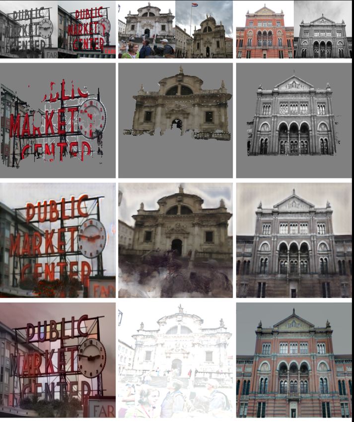
(a)                               (b)                         (c)                               (d)
Figure 1: Correspondences obtained with the CoAM model, which is augmented with an attention mechanism. These demonstrate
the model’s robustness in the face of challenging scene shift: changes in illumination (a,d), viewpoint (a-d), context (a,d), or style (b).

tasks: local matching, camera localization, 3D reconstruc-              hinge loss to enforce that true descriptors are nearby and
tion, and style transfer. We improve over state-of-the-art              false ones further away.
(sota) models, especially under challenging conditions, and             Dense correspondence matching with prior knowledge.
achieve sota or comparable on all tasks.                                Given a static scene and initial camera estimation, a sec-
    In summary, we present a key insight: that condition-               ond algorithm, e.g. PatchMatch [4, 68], can be used to find
ing learned descriptors on both images should allow for                 dense correspondences between the images and obtain a full
improved correspondence matching under challenging con-                 3D reconstruction. If the images have been rectified using
ditions. As will be seen, CD-UNet is simple and scalable and            multiple-view geometry [19] and have limited scene shift,
eschews a number of techniques used by other methods to                 stereo algorithms such as [17, 50, 73, 84] (and reviewed by
improve matching performance: high dimensional descrip-                 [74]) can be used to obtain a full 3D reconstruction.
tors (we use a 64D descriptor, half the size of the current                While not directly related, [26, 69] condition on a second
smallest descriptor), and multiple scales (we only operate at           image by iterative warping. This requires multiple passes
a single scale, whereas other methods use multiple scales).             through a network for each image pair and uses pre-trained
                                                                        descriptors as opposed to training end-to-end.
2. Related Work                                                            Also related are approaches that seek to learn correspon-
                                                                        dence between similar scenes [32] or instances of the same
   In this section, we review related work on finding corre-
                                                                        semantic class [26, 45, 55, 56].
spondences beyond the local descriptors discussed in Sec. 1.
                                                                        Local descriptors for image retrieval. Another form of
As there is a large amount of relevant research, we focus on
                                                                        correspondence is to find relevant images in a database using
the most relevant work in each category.
                                                                        a query image. Related works use an aggregation of local
Correspondences using an attention mechanism. Our ar-
                                                                        descriptors from a CNN [7, 78]. Again, these methods gen-
chitecture can be viewed as a generalization of the standard
                                                                        erate descriptors for the dataset images independently of the
correlation layer used in training end-to-end models for op-
                                                                        query image, whereas the descriptors we extract for the input
tical flow [12, 21, 72], stereo [25] or correspondence esti-
                                                                        image are conditioned on both images.
mation [11, 28, 64, 80, 81, 83]. This correlation layer (or
                                                                        Stylization for robust correspondence matching. Our
attention mechanism) is used to compute a cost volume of
                                                                        idea of conditioning the output of one image on another
matches from the learned descriptors.
                                                                        has interesting connections to stylization and associated gen-
   In correspondence estimation, the learned descriptors are
                                                                        erative models [23, 48, 79]. Additionally, a recent line of
limited in spatial resolution [28, 80, 83] so that the entire
                                                                        work studies how training on stylized images can improve
volume can be computed. This is too coarse for geometric
                                                                        robustness in correspondence matching [37]. As opposed to
matching, so other methods use a hierarchical approach
                                                                        enforcing invariance to style, CD-UNet and the other archi-
[11, 64, 81]. In optical flow [12, 21, 53, 72] and stereo [25],
                                                                        tectures considered, learn how to leverage differing styles
the cost volume is only applied within a limited support
                                                                        (as the precise style may be useful) via our CoAM.
region for a single descriptor (e.g. a square region or a raster
line) and typically at a lower resolution. Moreover, these
                                                                        3. Method
methods implicitly assume photometric consistency between
frames: their quality degrades the more the frames differ in                Our task is to find dense correspondences between a pair
time, as the pose and viewpoint progressively change.                   of images of the same scene. This proceeds in two stages.
   Unlike these methods, we apply attention at multiple                 The first stage obtains dense descriptor vectors for each
stages in our network, so that the final descriptors themselves         image and a distinctiveness score. The descriptors are con-
are conditioned on both images. This should be beneficial               ditioned on both images so they only have to be invariant
for challenging image pairs where one, final comparison                 to the changes particular to that pair of images. The second
is unable to encompass all possible scene-shifts between                stage compares these descriptor vectors to obtain a set of
two images. To find matches at the image level without                  high quality matches. We first describe in Sec. 3.1 our full
performing an exhaustive comparison, we use a modified                  architecture CD-UNet, and how it is trained in Sec. 3.2. CD-

                                                                    2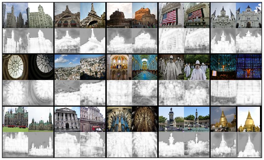
Figure 2: Overview of CD-UNet for obtaining co-attended descriptors. Descriptor vectors D1 for one input image I 1 are conditioned
on another I 2 using our CoAM. This module can be applied at multiple layers in the model hierarchy (we show one for clarity). The
conditioned features are then decoded to obtain D1 . We also regress a distinctiveness mask which is used at test time to ignore unmatchable
regions (e.g. the sky or regions visible in only one image). The descriptor vectors D2 for I 2 are obtained by swapping the input images.

UNet consists of a set of Co-Attention Modules (CoAMs)                   not be at the same spatial location. As a result, we use an
and a distinctiveness score regressor, which are incorporated            attention mechanism to model long range dependencies.
into a standard UNet architecture. Then, in Sec. 3.3, we de-                 In detail, the attention mechanism is used to determine
scribe how CoAM is incorporated into the recent CAPSNet                  where a location i in one set of features g from one image
architecture [81] and trained in a self-supervised manner.               should attend to in another set of features h from another
                                                                         image [80]. For each location i in g, it obtains a feature gˆi
3.1. A UNet encoder-decoder with CoAM                                    that is a weighted sum over all spatial features in h where A
    The architecture for obtaining descriptor vectors and a dis-         is the similarity matrix comparing g and h using the inner
tinctiveness score for one image I 1 (Fig. 2), is composed of            product followed by the softmax normalization step.
four components. The first component, the encoder, projects
both images I 1 , I 2 to obtain feature maps at two resolutions:
                                                                                        X                        exp(giT hj )
                                                                                ĝi =       Aij hj        Aij = P        T
                                                                                                                                        (1)
fLi , fSi . The second component, the attention mechanism                               j                        k exp(gi hk )
(CoAM), is used to determine spatial correspondence be-
tween the feature maps of the different images and obtain                    To apply this attention mechanism, we operate as follows
conditioned feature maps. The third component, the de-                   for fL1 (and similarly for fS1 ). First, to perform dimension-
coder, concatenates the conditioned feature maps with the                ality reduction (as is standard), the features are projected
original feature maps. These are decoded to obtain a grid                with two MLPs g 1 (·), g 2 (·): g = g 1 (fL1 ), h = g 2 (fL2 ). The
of spatial descriptor vectors D1 (which are conditioned on               attended features fˆL1 are then computed using the projected
both images). The final component, the regressor, learns a               features as in (1). This gives a new feature map of the fea-
distinctiveness score for each grid position, which encodes              tures in I 2 at the corresponding position in I 1 .
how likely the match is to be accurate. To obtain descriptor             Decoder: Conditioned Features. The attended features are
vectors D2 for the other image, we operate precisely as de-              incorporated into a UNet [59] architecture to obtain a grid of
scribed above, except that the order of the input images is              spatial descriptors D1 ∈ RH×W ×D (Fig. 2). The attended
flipped. This gives a grid of descriptor vectors D1 , D2 for             features fˆL1 and fˆS1 are concatenated with the original fea-
images I 1 , I 2 respectively.                                           tures and passed through the decoder portion of the UNet.
Encoder. Given two images of the same scene, I 1 ∈                       The resulting feature map is L2 normalized over the channel
RH×W ×3 and I 2 ∈ RH×W ×3 , we obtain spatial feature                    dimension to obtain the final descriptors. This step ensures
maps: fLi and fSi at a larger and smaller resolution. These              that the final descriptors are conditioned on both images.
will be concatenated within a UNet framework [59] and in-                Regressor: Distinctiveness Score. We regress a distinc-
jected into the decoder. A CNN with shared parameters is                 tiveness score r(·)ij ∈ [0, 1], for each pixel (i, j), which
used to encode the images and obtain these spatial feature               approximates its matchability and is used at test time to se-
maps. In practice, we use the feature maps after the last two            lect the best matches. r(·)ij approximates how often the
blocks in a ResNet50 [20] architecture.                                  descriptor at (i, j) is confused with negatives in the other
CoAM Attention Module. We wish to concatenate features                   image. If it is near 1, the descriptor is uniquely matched; if
from both images in order to condition the model on both                 it is near 0, the descriptor is often confused. To regress these
input images. However, for a given spatial location, the                 values, we use an MLP, r(·), on top of the unnormalized
relevant (corresponding) feature in the other image may                  descriptor maps.

                                                                     3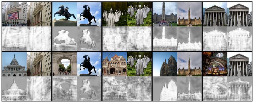
Determining Matches at Test Time. We want matches at                    Distinctiveness Loss. To learn the r(·) MLP, we need an
locations k and l in images I 1 and I 2 respectively that are           estimate of how often a descriptor in one image is confused
accurate and distinctive (e.g. no matches in the sky). We               with the wrong descriptors in the other image. Given a set N
use the scalar product to compare the normalized descriptor             of N negative matches in the other image and the margin M ,
vectors to find the best matches and the distinctiveness score          the number   P of times a descriptor at location x is confused
to determine the most distinctive matches. The following                is mx = ŷ∈N 1(d(Dx1 , Dŷ2 ) < M ). This value is used to
similarity score ckl combines these properties such that a              regress r(·), which is near 1 if the feature has a unique match
value near 1 indicates a distinct and accurate match:                   (the true match), near 0 otherwise (τ is a hyper-parameter
                                  h     T     i                        set to 14 ):
              ckl = r(Dk1 )r(Dl2 ) Dk1 Dl2 .               (2)
                                                                                          1 X               1
   Finally, we select the best K matches. First, we exhaus-                        Lr =       |r(Dx1 ),            |1 .             (6)
                                                                                          L             (1 + mx )τ
tively compare all descriptors in both images. Then, we                                     (x,·)∈P

only select those matches that are mutual nearest neighbours:
e.g. if the best match for location m in one image is location          Training Setup. CD-UNet is trained on MegaDepth [31],
n in another, and the best match for location n is m, then              which consists of a variety of landmarks, registered using
(n, m) is a good match. So if the following holds:                      SfM [66]. As each landmark consists of many images taken
                                                                        under differing conditions, we can obtain matches between
      m = argmaxj cnj            and n = argmaxi cim .        (3)       images that are unmatchable when considered independently.
                                                                           We train the features end-to-end, but train the distinctive-
These matches are ranked according to their similarity score            ness score separately by not allowing gradients to flow. In
and the top K selected.                                                 practice we backpropagate on all randomly chosen positive
3.2. Supervised Training and Loss Functions                             pairs Lp , negative pairs Ln , and additionally the hardest
                                                                        H = 3 negative pairs for each positive pair.
Selecting Correspondences at Train Time. Given a                           The model is trained with a learning rate of 0.0001, the
ground-truth correspondence map, we randomly select L                   ADAM optimizer [27], a batch size of 16, M =1, L=512, and
positive correspondences. For each positive correspondence,             N =512. At train time we use an image size of 256, at test
we randomly select a large number (N = 512) of nega-                    time an image size of 512. We use K=2000 for HPatches
tive correspondences. These randomly chosen positive and                and Aachen, and K=8192 when performing SfM. For SfM,
negative correspondences are used to compute both the dis-              we find it is important to use more, rougher correspondences
tinctiveness and correspondence losses.                                 to obtain more coverage in the 3D reconstruction.
Correspondence Loss. The correspondence loss is used
to enforce that the normalized descriptor maps D1 and D2                3.3. Self-supervised training – the CAPSNet [81]
can be compared using the scalar product to obtain the best                   with CoAM
matches. At a location i in D1 and j in D2 then the standard
                                                                            In this section we describe how CoAM can be added
Euclidean distance metric d(Di1 , Dj2 ) should be near 0 if the
                                                                        to the CAPSNet architecture of [81] and trained using the
corresponding normalized descriptor vectors are a match.
                                                                        self-supervised framework of [81].
   To train these descriptors, we use a standard contrastive
                                                                            CAPSNet consists of a UNet style architecture, which
hinge loss to separate true and false correspondences (we
                                                                        predicts features at a coarse and fine level. The matches at a
consider other contrastive losses in the appendix). For the
                                                                        coarse level are used to guide feature matching at the finer
set P of L true pairs, the loss Lp enforces that the distance
                                                                        level. These features are trained using two losses. First, an
between descriptors is near 0. For the set N of LN nega-
                                                                        epipolar loss enforces that matches should satisfy epipolar
tive pairs, the loss Ln enforces that the distance between
                                                                        constraints. Second, a cycle consistency loss enforces that,
descriptors should be above a margin M .
                                                                        for a match between two images, the best match for the local
          1    X                                                        descriptor in one image should also be the best match for
   Lp =                 d(Dx1 , Dy2 )                         (4)       the local descriptor in the other. Using this approach, the
          L
              (x,y)∈P
                                                                        authors achieve high quality results at pose estimation on the
           1      X
                                                                        challenging MegaDepth test set.
  Ln =                     max(0, M + cx − d(Dx1 , Dŷ2 )).   (5)
          LN                                                                As the descriptor model is a UNet style architecture, and it
                (x,ŷ)∈N
                                                                        is trained in an end-to-end fashion, we operate in a very sim-
   cx = d(Dx1 , Dy2 ), (x, y) ∈ P re-weights the distance of            ilar manner to the UNet architecture with CoAM of Sec. 3.1,
the false correspondence according to that of the positive one:         by again adding CoAMs to condition descriptors on both
the less confident the true match, the further the negative one         images. We use the CoAM to inject attended features from
must be from M [10].                                                    the other image at either a coarse level or at a fine and coarse

                                                                    4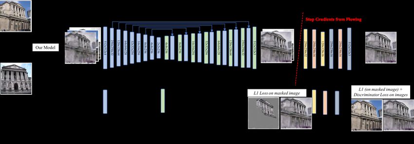
Method                         # Matches
                                                                                             Hes. det. + RootSift [1, 33]     2.8K
                                                                                             HAN + HN++ [41, 40]              2.0K
                                                                                             LF-Net [46]                      0.2K
                                                                                             SuperPoint [9]                   0.9K
                                                                                             DELF [44]                        1.9K
                                                                                             D2 Trained (SS) [10]             2.5K
                                                                                             R2D2 [54]                        1.8K
                                                                                             Ours                             2.0K

Figure 3: HPatches [2]. Comparison with sota using the mean matching accuracy for different pixel thresholds on the HPatches dataset.
We also report the mean matches extracted per image pair. For this dataset, one desires more matches with high accuracy. Our method
achieves superior performance when images vary by illumination for all thresholds, and by viewpoint for thresholds > 6px. By a simple
refinement strategy (ours (ref)), we achieve sota for all thresholds on both viewpoint and illumination.

level (precise details are given in the appendix). In both           4. Experiments I: Supervised Co-AM
cases, this leads to an addition of less than 15% of the total
weights of the original network.                                         In this section we evaluate the CD-UNet architecture
                                                                     (UNet encoder-decoder with CoAM and distinctiveness
   The loss functions used to train the conditioned local            score as in Fig. 2) on four challenging downstream tasks un-
descriptors are unchanged from the original CAPSNet work.            der full supervision. In Sec. 5 the benefits of the co-attention
Training Setup. We train the model as done in [81]: for              module are evaluated under self-supervised training [81].
200K iterations, using a batch size of 6 images, and an image            The first task directly assesses how well CD-UNet can
size of 480 × 640.                                                   estimate correspondences between images pairs. The second
                                                                     task uses the correspondences to perform camera localiza-
                                                                     tion. In these tasks we ablate the utility of the CoAM and
3.4. Discussion                                                      distinctiveness score components of the architecture. The
                                                                     third task obtains high quality 3D reconstructions in chal-
    Here we discuss some of the benefits of conditioning             lenging situations, with a large amount of scene shift. The
using CoAM as opposed to operating directly on local de-             final task is stylization, and assesses CD-UNet’s matches,
scriptors and keypoints as done in SuperGLUE [61]. First,            when extracted in a dense manner, on a downstream task.
our module is trained end-to-end and does not introduce                  In general we find that CD-UNet achieves state of the
an extra step in the matching pipeline of comparing pre-             art or comparable results and that the CoAM is useful espe-
trained descriptors. Second, our descriptors are learned,            cially in challenging conditions (e.g. when there is a large
so our method is not dependent on the quality of the ex-             viewpoint change).
tracted descriptors. Finally, SuperGLUE scales with the                  The appendix includes further ablations to validate our
number of extracted keypoints, hampering its performance             choices (e.g. the loss function and grid size) and datasets
and utility on tasks that require finding a large number of          (e.g. (1) YFCC100M [76] which shows our superior re-
correspondences (e.g. SFM). As the CoAM is plugged in as             sults and the utility of both the distinctiveness score and
a component of our network, our method scales with image             the CoAM, and (2) a new, challenging SFM dataset). Finally,
size. For reference, on a single GPU, to extract 2k keypoints        it includes qualitative samples for each of the experiments
on a 256 × 256 image, our method runs in 97ms while Su-              discussed in the following, including HPatches, Aachen,
perGLUE would add an overhead of ≈270ms as reported                  SFM, and stylization.
in the original paper. Further, our method would scale with          Ablations. The full model uses the ResNet50 [20] backbone,
little overhead to more keypoints at the given image size.           the CoAMs and the distinctivness score to reweight matches.
   Our method requires an exhaustive match of all image              We ablate multiple variants. The first (ours) is our full
pairs. While we find that we can run the full, exhaustive            model. The second (ours w/o conf) is our model without the
pipeline on reasonably large datasets (≈ 1500 images) in             distinctiveness score but only the scalar product. The third
Sec. 4.2.2, we envision two stages when using our method             (ours w/o cond) is our model without conditioning (i.e. the
in truly large scale settings. First, a coarser, faster method       CoAMs). The final variant (ours-E-B1) is our full model but
can be used as a preprocessing step to remove spurious pairs         using an EfficientNet-B1 backbone [75]. This ablation uses
and our method subsequently used in a second stage to find           a smaller (7M params vs 23M params) and faster (0.7GFlops
high quality correspondences.                                        vs 4.1GFlops) backbone architecture; it is more suitable for

                                                                 5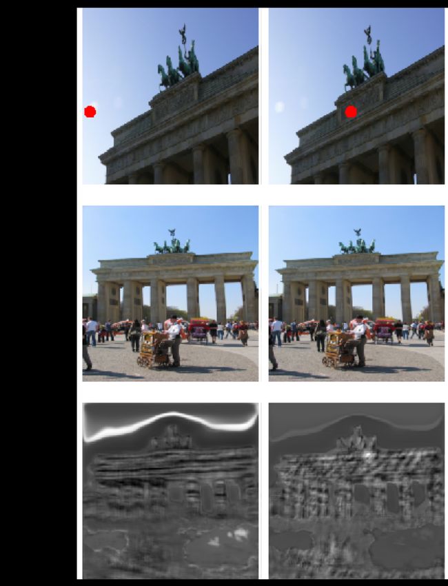
Table 1: Aachen Day-Night [62]. Higher is better. Ours does                  Table 2: SfM. We compare our approach to using SIFT features
comparably or better than other sota setups. ∗ indicates the method          on 3D reconstruction. ↑: higher is better. ↓: lower is better.
was trained on the Aachen dataset.
                                                                                                                             Large SfM
      Method                            Threshold Accuracy                                        Landmark:    Madrid Met.     Gen.      Tow. of Lon.
                              0.25m (2◦ )     0.5m (5◦ )     5m (10◦ )                            SIFT [33]:      500          1035          804
                                                                                # Reg. Ims ↑
      Upright RootSIFT [33]      36.7           54.1           72.5                                   Ours:       702          1072          967
      DenseSFM [62]              39.8           60.2           84.7                               SIFT [33]:      116K         338K         239K
      Han+, HN++ [41, 40]        39.8           61.2           77.6             # Sparse Pts ↑
                                                                                                     Ours:        256K         570K         452K
      Superpoint [9]             42.8           57.1           75.5
      DELF [44]                  39.8           61.2           85.7                               SIFT [33]:      6.32         5.52         7.76
                                                                                Track Len ↑
      D2-Net [10]                44.9           66.3           88.8                                  Ours:        6.09         6.60         5.82
      R2D2* [54]                 45.9           66.3           88.8
                                                                                                  SIFT [33]:      0.60         0.69         0.61
                                                                              Reproj Err (px) ↓
      Ours w/o cond              42.9           62.2           87.8                                  Ours:        1.30         1.34         1.32
      Ours w/o conf              43.9           64.3           86.7
                                                                                                  SIFT [33]:      1.8M         4.2M         3.1M
      Ours                       44.9           70.4           88.8             # Dense Pts ↑
                                                                                                     Ours:        1.1M         2.1M         1.8M
      Ours (E-B1)                44.9           68.4           88.8

                                                                             olds for viewpoint and illumination changes. Compared to
practical applications.                                                      the other evaluation datasets, e.g. [62] below, the compo-
                                                                             nents of our model have a limited impact on performance
4.1. Correspondence Evaluation
                                                                             on this benchmark, presumably because this dataset has less
    We test our model on local matching by evaluating on                     scene shift than the others.
the HPatches [2] benchmark. We compare to a number of
baselines and achieve state-of-the-art results.                              4.2. Using Correspondences for 3D Reconstruction
HPatches Benchmark. The HPatches benchmark evaluates
                                                                                In this section, we evaluate the robustness of our approach
the ability of a model to find accurate correspondences be-
                                                                             on images that vary significantly in terms of illumination and
tween pairs of images, related by a homography, that vary
                                                                             viewpoint, and our model’s ability to scale to larger datasets.
in terms of illumination or viewpoint. We follow the stan-
                                                                             CD-UNet achieves sota or comparable results on all datasets.
dard setup used by D2Net [10] by selecting 108 of the 116
sequences which show 6 images of larger and larger illumi-
nation and viewpoint changes. The first image is matched                     4.2.1    Camera Localization
against the other 5, giving 540 pairs.
Evaluation Setup. We follow the evaluation setup of D2Net                    Aachen Benchmark. In order to evaluate our approach
[10]. For each image pair, we compute the number of cor-                     under large illumination changes, we use the Aachen Day-
rect matches (using the known homography) and report the                     Night dataset [62, 63]. For each of the 98 query night-time
average number of correct matches as a function of the pixel                 images, the goal is to localize the image against a set of
threshold error in Fig. 3. We then compare to a number                       day-time images using predicted correspondences.
of detect-then-describe baselines used in D2Net using their                  Evaluation Setup. The evaluation measure is the percentage
software: RootSIFT [1, 33] with the Affine keypoint detec-                   of night time cameras that are localized within a given error
tor [38], HesAffNet [41] with HardNet++ [40], LF-Net [46],                   threshold [62]. We use the pipeline and evaluation server
SuperPoint [9], DELF [44]; as well as to D2Net [10] and                      of [62] with the matches automatically obtained with our
R2D2 [54]. These methods vary in terms of whether the                        method (Sec. 3.1). We compare against RootSIFT descrip-
detector and descriptors are hand crafted or learned.                        tors from DoG keypoints [33], HardNet++ with HesAffNet
Results. As shown in Fig. 3, all variants of our model outper-               features [40, 41], DELF [44], SuperPoint [9], D2Net [10]
form previous methods for larger pixel thresholds, demon-                    and DenseSFM [62].
strating the practicality and robustness of our approach. In                 Results. Tab. 1 shows that our method does comparably
comparison to other methods, CD-UNet performs extremely                      or better than other sota approaches. They also show the
well when the images vary in illumination: it outperforms                    utility of the distinctiveness score and CoAM. These results
all other methods. CD-UNet is superior under viewpoint                       imply that the traditional approach of first finding reliably de-
changes for larger pixel thresholds (> 6px). Using the                       tectable regions may be unnecessary; using a grid to exhaus-
smaller, more efficient (ours-E-B1) actually improves per-                   tively find matches is, perhaps surprisingly, superior in this
formance over the larger ResNet model (ours). A simple                       case. These results also show that our architectural improve-
refinement strategy (described in the appendix) boosts our                   ments (i.e. using an attention mechanism and distinctiveness
model’s performance under viewpoint changes, giving re-                      score) boost performance and that an efficient architecture
sults superior or comparable to sota methods for all thresh-                 (Ours-E-B1) has a small impact on performance.

                                                                         6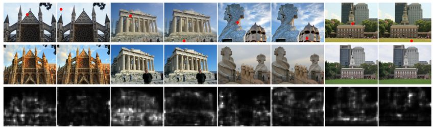
Inputs
(Iv , Is )                                                                    I1

                                                                              I2
  GTS

                                                                              A

  Ours
                                                                           Figure 5: CoAM Attention. We visualize the predicted attention
                                                                           (A) for sample image pairs. The red dot in I 1 denotes the point
                                                                           for which we compute the attention. It is not clear apriori what the
                                                                           attention module should do, but it does attend to relevant, similar
                                                                           regions in the other image and is dependent on the query location.
  [34]

                                                                           However, clearly our results are competitive with SIFT.
                 (a)             (b)              (c)
                                                                           4.3. Using Correspondences for Stylization
 Figure 4: Stylization. Given Is and Iv , the task is to generate an
                                                                              Previously, we focused on using our matching pipeline for
 image with the pose and viewpoint of Iv and style of Is . We show
 results for CoAM and a baseline that uses semantics [34]. We also
                                                                           extracting a set of correspondences to be used for localization
 show the resampled image (GTS ) which is computed using the               and 3D reconstruction. Here we evaluate how well our
 true correspondences from the MegaDepth dataset [31]. While [34]          features can be used for a task that requires dense matching:
 works well for easy cases, it sometimes copies style from Iv (as          stylization. The goal is, given two images Is , Iv of the same
 shown by the red background in (a) and red hued building in (c)).         scene, to generate an image with the style of Is but the pose
 [34] also fails if the semantic prediction is incorrect (e.g. (b)).       and viewpoint of Iv .
                                                                           Setup. To achieve this, we first use CD-UNet to transform
                                                                           Is into the position of Iv . The approach is simple: instead
 4.2.2       Structure from Motion (SfM)                                   of only choosing the mutual nearest neighbours as in (2),
                                                                           we consider the best match for every pixel location. Then,
 The objective here is to evaluate the correspondences ob-                 the color of the best match in Is is used to color the corre-
 tained with our model for the task of 3D reconstruction.                  sponding location in Iv . This gives the sampled image. The
 SfM Dataset. The assessment is on the standard SfM                        next step is to remove artefacts. We do this by training a
 Local Feature Evaluation Benchmark [67] that contains                     refinement model on top of the sampled image in order to
 many (≈ 1500) internet images of three landmarks: Madrid                  obtain an image Ig in the pose of Iv and style of Is . Full
 Metropolis, Gendarmenmarkt, and Tower of London.                          details of the architecture and training are given in the supp.
 Baselines. We compare to SIFT [33]. This method first                     Relation to Pix2Pix [22]. In a standard image to image
 finds repeatably detectable regions for which features are                translation task (e.g. Pix2Pix [22]), the two images (e.g. im-
 extracted and compared between images. This method works                  age and semantic map) are aligned. In our case, the images
 well when there are distinctive textured regions that can                 are not aligned. We effectively use our correspondences to
 be found and matched. Our method, however, conditions                     align the images and then run a variant of Pix2Pix.
 on both images, so our approach should be more robust                     Experimental Setup. To evaluate our results, we use the
 when there are fewer textured regions or where there are                  test set of the MegaDepth dataset (these are landmarks un-
 significant variations between the images as it can make use              seen at training time). We randomly select 400 pairs of
 of auxiliary information from the other image. Additional,                images and designate one the viewpoint Iv image and the
 less challenging baselines are given in the appendix.                     other the style image Is . We task the models to generate
 Results. Tab. 2 shows that, using CD-UNet, we consistently                a new image Ig with the style of Is in the viewpoint of Iv .
 register more images and obtain more sparsely reconstructed               From the MegaDepth dataset, we can obtain ground truth
 3D points (visualizations are in the appendix). However, the              correspondence for regions in both images and so the true
 pixel error is higher and there are fewer dense points. These             values of Ig for this region. The reported error metric is
 differing results are somewhat explained by the implicit trade            the mean L1 distance between the generated image and true
 off between number of points and reprojection error [81].                 value within this region.

                                                                       7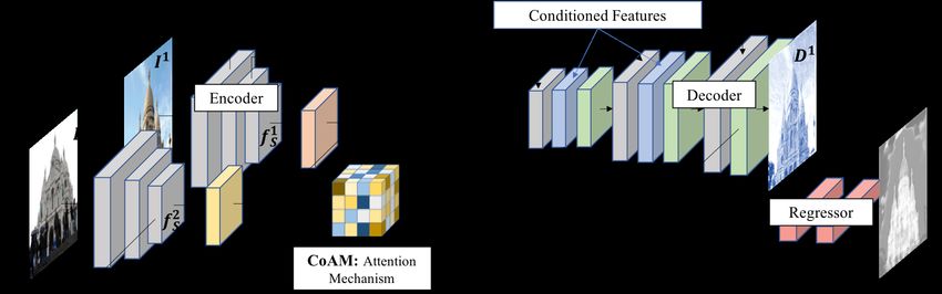
Method                   Accuracy on MegaDepth                        We consider two variants of injecting CoAM into the
                                easy      medium       hard                 CAPSNet architecture. First, (C CoAM) only injects one
   CAPS [81] w/ SIFT Kp.     91.3 / 52.7   82.5 / 57.9   65.8 / 61.3        CoAM at a coarse resolution. Second, (C+F CoAM) injects
      Ours (C CoAM)          91.7 / 52.1   82.9 / 58.6   69.3 / 62.4        two CoAMs at a coarse and a fine resolution. We report
     Ours (C+F CoAMs)        91.9 / 52.3   82.8 / 58.4   68.8 / 63.4        the percentage of correct images for rotational and transla-
                                                                            tional errors separately in Tab. 3. These results demonstrate
Table 3: Results on the MegaDepth dataset on three increasingly             that using a CoAM does indeed improve over the baseline
challenging subsets (easy, medium, and hard) for both angular /             model, especially on the harder angle pairs. Injecting fur-
translational errors: (·) / (·). The results show that augmenting the       ther CoAMs does not substantially increase performance but
baseline model with our CoAMs improves performance, especially
                                                                            it consistently performs better than the original CAPSNet
on the challenging viewpoint images, demonstrating the utility of
conditioning the descriptors on both images under these conditions.
                                                                            model. This demonstrates the value of using our CoAM to
                                                                            condition descriptors on both images.

Results. We compare against a stylization approach that                     5.2. Visualisation of CoAM’s Attention
uses semantics to perform style transfer [34] in Fig. 4. We
also determine the L1 error for both setups and obtain 0.22                     Finally, we visualize CoAM’s predicted attention in Fig. 5
for [34] and 0.14 for our method, demonstrating that our                    to obtain an intuition of how the additional image is used
method is more accurate for regions that can be put in cor-                 to improve the learned descriptors. We note that there is no
respondence. The qualitative results demonstrate that our                   clear a priori knowledge of what the model should attend to.
method is more robust, as [34] produces poor results if the                 The attention module could find regions of similar texture
semantic prediction is wrong and sometimes copies style                     but varying style in order to be invariant to the style. Or
from Iv as opposed to Is (e.g. it creates a colored Ig image                the module could attend to the right location in the other
when Is is grey-scale). As we sample from Is in the first step              image. However, the qualitative results imply that the model
and then refine the sampled image, our model rarely copies                  is making use of the CoAM to attend to relevant regions.
style from Iv . Finally, our full method runs in seconds at test                Additionally, we quantify how invariant the descriptors
time whereas [34] takes minutes due to a computationally                    are with the CoAM and without. We use the sets of images in
intensive iterative refinement strategy.                                    the HPatches benchmark that vary in illumination. One im-
                                                                            age is kept fixed (the target) and the other varied (the query).
5. Experiments II: CoAM with CAPSNet                                        We then evaluate how much the query image’s descriptors
                                                                            vary from those of the target by computing the L1 error.
   Next, we evaluate CoAM when injected into the CAP-
                                                                            Our descriptors differ on average by 0.30 ± 0.14, whereas
SNet architecture [81] and trained in a self-supervised man-
                                                                            [81]’s descriptors differ more, by 0.41 ± 0.17. This validates
ner. We again validate our hypothesis that conditioning on
                                                                            that the CoAM increases the invariance of corresponding
two images is preferable in this setting, as it improves re-
                                                                            descriptors under large amounts of scene shift.
sults on the downstream task of pose prediction. Finally, we
visualize and investigate the learned attention to obtain an
intuition into how CoAM is being used by the network.                       6. Conclusion
5.1. Camera Pose Prediction                                                    We investigated a new approach for obtaining correspon-
    This experiment follows that of [81]. The aim is to es-                 dences for image pairs using a co-attention module and dis-
timate the relative camera pose between pairs of images                     tinctiveness score. The central insight was that, using neural
extracted at random from the MegaDepth test set. The pairs                  networks, descriptors can be conditioned on both images.
of images are divided into three subsets depending on the rel-              This allows greater flexibility, as the descriptors only need
ative angular change: easy ([0◦ , 15◦ ]), medium ([15◦ , 30◦ ]),            to be invariant to changes between the pair of images. Us-
and hard ([30◦ , 60◦ ]). Each subset has at least 1000 pairs.               ing this insight, our simple model improved the quality of
    In order to determine the relative camera pose, we follow               the learned descriptors over those of a baseline model on
the approach of [81]. The essential matrix is extracted by                  multiple tasks and in both a supervised and self-supervised
using the mutual nearest neighbour correspondences and                      setting. We would expect further improvements with larger,
known camera intrinsic parameters. The essential matrix is                  more complex models.
decomposed into the rotation and translation matrices. The                  Acknowledgements. The authors thank Noah Snavely and
estimated angular change in rotation and translation is then                David Murray for feedback and discussions. This work
compared to the ground truth. If the difference between the                 was funded by an EPSRC studentship, EPSRC Programme
predicted and ground truth is less than a threshold of 10◦ ,                Grant Seebibyte EP/M013774/1, a Royal Society Research
the prediction is considered correct.                                       Professorship, and ERC 638009-IDIU.

                                                                        8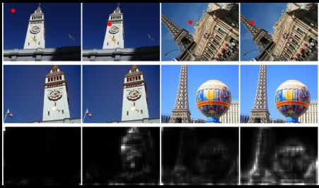
A. Overview
   We include additional implementation details and results
in Sec. B. These experiments demonstrate the following.
First, the importance of both the distinctiveness score and
CoAM to achieve sota results with comparison to other sin-
gle stage approaches on the challenging YFCC100 dataset.
Second, they demonstrate how our approach can use a refine-
ment step to achieve state-of-the-art results for all thresholds
>1px on HPatches. Third, they provide additional ablations             Figure 6: Results on HPatches when refining correspondences.
including the use of a Noise Contrastive (NCE) loss as op-             In this experiment, we look at the results of using a refinement strat-
                                                                       egy based on a local neighbourhood to improve the accuracy of the
posed to the hinge loss presented in the paper. Finally, we
                                                                       detected correspondences. We see that using the refinement scheme,
provide more results and explanation for the SfM results
                                                                       we obtain a big boost in performance. In particular, we improve
given in the main paper. We define the metrics used in ob-             our results for fine-grained pixel thresholds on the viewpoint task.
taining the SfM results in Sec. B.3 and provide additional             We achieve comparable results with state-of-the-art methods for
baselines. We also demonstrate that our model is more robust           small pixel thresholds and better performance for larger thresholds
than the one using SIFT on a challenging, new dataset of               (> 4px). On illumination we maintain performance except for very
Henry Moore sculptures. Finally, we provide visualisations             small thresholds (≤ 1px). This small degradation is probably due
of our reconstructed 3D models here and in the attached                to limited noise that is introduced with the refinement strategy. In
video.                                                                 general, using this strategy we improve our results to achieve state
   Additionally, we provide further details of the architec-           of the art performance for all pixel thresholds.
tures used in Sec. C for the CD-UNet, CoAM + CAPSNet
[81], and the stylization model.
                                                                       dataset in Tab. 7 but obtained comparable results to using
   We also provide qualitative samples of the distinctive-
                                                                       G = 128. As a result, we continued to use G = 128 for all
ness scores learned by our model in Sec. D.2. We provide
                                                                       our experiments. Using a larger grid for the larger datasets in
additional qualitative results for the stylization experiment,
                                                                       SfM (where the number of images are approximately 1500)
HPatches dataset, SfM experiment, and Aachen dataset in
                                                                       would have made these experiments intractable using current
Sec. D.3.
                                                                       pipelines.
                                                                          However, we note that because we only consider points
B. Additional Experiments
                                                                       on a grid, we are losing some granularity which presum-
   In this section we report the results of additional exper-          ably impacts the performance on the 3D reconstruction tasks.
iments which consider additional ablations of the grid size            We discuss a method to refine the correspondences to ob-
chosen at test time (Sec. B.1), a refinement of our model to           tain a finer granularity in the next section and the resulting
improve local matching (Sec. B.2) to achieve state-of-the-             complications.
art results on HPatches, further comparisons of our model
on the 3D reconstruction task (Sec. B.4.1), results on the             B.2. Refining Local Matching
YFCC100M dataset (Sec. B.5), and results using another                     In this section, we demonstrate that our local matching re-
popular contrastive loss (NCE) (Sec. B.6).                             sults can be improved by using a simple refinement strategy.
                                                                           Description of Refinement Strategy. In order to refine
B.1. Further Ablations
                                                                       the matches obtained using CD-UNet, we use a local neigh-
   In this section we discuss and ablate how we select candi-          bourhood to refine the match in the second image. Given a
date matches at test time.                                             correspondence with location (x1 , y1 ) in the first image and
   In order to compare all descriptor vectors at test time, we         (x2 , y2 ) in the second image, we look at the similarity score
operate as follows. We create a G × G pixel grid and bilin-            between (x1 , y1 ) and the locations in a 3x3 grid centered on
early interpolate on this grid from both the descriptor maps           (x2 , y2 ).
and distinctiveness scores. (Note that we have to normalize                These scores are used to reweight the location in the
the interpolated descriptors.) We consider all pairs of de-            second image using a normalized weighted sum with one
scriptors as candidate matches and compare all descriptors in          difference. Because the similarity scores are not evenly
one image to those in the other. In practice we use G = 128.           distribute and cluster around 0.5, they give too much weight
   At test time, we could use a larger grid size for better            to less likely matches. As a result, we subtract the minimum
granularity. However, this comes with the additional com-              similarity from all scores in a local neighbourhood before
putational cost of performing G4 comparisons. We tried                 computing the normalized weighted sum.
using a larger grid (G = 256) on the Aachen-Day Night                      Results. The results are given in Fig. 6. As can be seen,

                                                                   9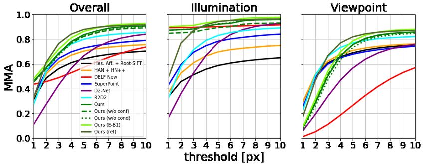
this simple refinement scheme gives a large boost in perfor-                  indicates that the model is more robust, as more images
mance. In particular, using this simple modification gives                    see that 3D point.
superior results to state of the art approaches for pixel thresh-
olds > 4px for viewpoint and all thresholds > 2px for illu-                4. ↓ Reproj err: The repreojection error. This is the av-
mination. Overall, our model with the refinement scheme                       erage pixel error between a 3D point and its projection
achieves state-of-the-art results for all thresholds > 1px.                   in the images. If this is lower, it indicates the 3D points
    Discussion. While we could achieve high quality per-                      are more accurate.
formance on HPatches using this simple modification, we
note that it is not straightforward to apply this to the cam-              5. ↑ # Dense Points: The number of dense points. This
era localization or 3D reconstruction tasks. This is because                  is the number of dense points in the final 3D model.
both of these tasks require a single point to be tracked over                 The higher this is, the more of the 3D structure was
multiple images in order to perform 3D reconstruction (the                    able to be reconstructed.
camera localization performs 3D reconstruction as part of
the evaluation pipeline). 3D reconstruction pipelines assume
a detect and describe pipeline for extracting matches, which             B.4. Further Results for SfM
implicitly have this assumption baked in to their setup, as                  We include additional baselines on the Local Feature
they match the same detected points across different images.             Evaluation Benchmark of the original paper. We additionally
    However, this assumption is not implicit to our approach,            include results in a challenging scenario where the dataset
as we only find correspondences between pairs of images at               contains fewer (≈ 10 − 100 images) images of the same
a time. Further refining the points means that the location of           scene and where the object (a sculpture) may differ in mate-
a refined point from one pair of images will not necessarily             rial, location, and context.
match that of another pair, invalidating the track and nega-
tively affecting the 3D reconstruction. Incorporating these
refined points would require rethinking how we incorpo-                  B.4.1   Further Baselines on Local Feature Evaluation
rate refined correspondences in a 3D reconstruction pipeline.                    Benchmark
For example, we could use a reference image against which                In this section we compare our 3D reconstruction on the
further images are compared and incorporated. Once a ref-                Local Feature Evaluation Benchmark [67] to two additional
erence image has been exhausted, a new reference image                   baselines [10, 36] in Tab. 4. These results were not included
would be chosen and so on. We leave such an investigation                in the paper as these additional baselines perform similarly
to future work, but the boost in performance demonstrates                to SIFT [33] and there was limited space. However, we
the further potential of our setup.                                      note that both of these baselines use learned descriptors, yet
B.3. SfM Terminology                                                     they do not perform any better than SIFT in terms of the
                                                                         number of registered images and sparse 3D points. Our
   Here we define the metrics used in reporting the SfM                  method performs significantly better across all three large
results. Note that these metrics are only indicative of the              scale datasets for obtaining sparse 3D points and registering
quality of the 3D model; please look at the reconstructed                images.
models in the zipped video for a qualitative estimate as to
their respective quality.
                                                                         B.4.2   Further Results on a Sculpture SFM Benchmark
  1. ↑ # Reg. Ims: The number of registered images. This                 We use images from the Sculpture dataset [14], which con-
     is the number of images that are able to be put into                sists of images of the same sculpture downloaded from the
     correspondence and for which cameras were obtained                  web. As an artist may create the same sculpture multiple
     when doing the 3D reconstruction. A higher values                   times, a sculpture’s material (e.g. bronze or marble), location,
     means more images were registered, implying a better                or context (e.g. the season) may change in the images (refer
     model.                                                              to the supplementary for examples). In particular, we evalu-
  2. ↑ # Sparse Pts: The number of sparse points. This is                ate on nine sculptures by the artist Henry Moore. These sets
     the number of sparse points obtained after performing               of images contain large variations and the sculpture itself is
     the 3D geometry estimation. The higher the number                   often smooth, leading to less texture for finding repeatably
     indicates a better model, as more correspondences were              detectable regions.
     able to be triangulated.                                                We report the results in Tab. 5 and visualise samples in
                                                                         Fig. 15. While these metrics are proxies for reconstruction
  3. ↑ Track Len: The track length. How many images a                    accuracy, our approach is able to consistently obtain more
     given 3D point is seen in on average. If this is higher, it         3D points than the others for each image set. These results

                                                                    10
Table 4: SfM. We compare our approach to three baselines on 3D reconstruction for three scenes with a large number of images. Our
method obtains superior performance across the metrics except for reprojection error, despite using coarse correspondences and a single
scale. In particular, our method registers more images and obtains more sparse 3D points. ↑ denotes higher is better. ↓ denotes lower is
better.
LMark Method ↑ # Reg. Imgs ↑ # Sparse Pts ↑ Track Len ↓ Reproj. Err ↑ # Dense Pts
Madrid RootSIFT [33] 500 116K 6.32 0.60px 1.82M
Metropolis GeoDesc [36] 495 144K 5.97 0.65px 1.56M
1344 images D2 MS [10] 495 144K 6.39 1.35px 1.46M
Ours 702 256K 6.09 1.30px 1.10M
Gendarmen- RootSIFT [33] 1035 338K 5.52 0.69px 4.23M
markt GeoDesc [36] 1004 441K 5.14 0.73px 3.88M
1463 images D2 MS [10] 965 310K 5.55 1.28px 3.15M
Ours 1072 570K 6.60 1.34px 2.11M
Tower of RootSIFT [33] 804 239K 7.76 0.61px 3.05M
London GeoDesc [36] 776 341K 6.71 0.63px 2.73M
1576 images D2 MS [10] 708 287K 5.20 1.34px 2.86M
Ours 967 452K 5.82 1.32px 1.81M
Table 5: SfM. We compare our approach to using SIFT features on 3D reconstruction on a challenging new SFM dataset of sculptures.
This dataset contains images from the web containing large variations in illumination and viewpoint. These metrics are a proxy for 3D
reconstruction quality, so we encourage the reader to view the reconstructions in the supplementary. X: failure. ↑: higher is better. ↓: lower
is better.
Sculpture Dataset
Landmark: HM1 HM2 HM3 HM4 HM5 HM6 HM7 HM8 HM9
# Images: 12 124 250 266 78 31 358 238 74
SIFT [33]: X 103 198 212 61 22 266 201 53
# Reg. Ims ↑
Ours: 12 108 194 215 67 25 284 201 57
SIFT [33]: X 48K 70K 102K 28K 9K 128K 99K 23K
# Sparse Pts ↑
Ours: 2.9K 63K 83K 121K 40K 10K 190K 99K 21K
SIFT [33]: X 5.33 5.92 5.80 4.54 4.73 4.46 5.24 4.75
Track Len ↑
Ours: 3.60 5.03 5.43 5.61 4.32 4.00 4.23 5.24 4.77
SIFT [33]: X 1.31 1.32 1.28 1.30 1.33 1.22 1.30 1.32
Reproj Err (px) ↓
Ours: 1.33 1.30 1.30 1.29 1.29 1.26 1.23 1.30 1.32
SIFT [33]: X 160K 143K 307K 73K 46K 174K 333K 54K
# Dense Pts ↑
Ours: 0.2K 188K 156K 296K 82K 44K 187K 333K 53K
validate that our approach does indeed make our model ro- extract high quality matches for each pair of images. We
bust in this context and it performs as well if not better than use the known intrinsics to convert these to points in camera
the SIFT baseline method. space. We then use RANSAC [13] and the 5-point algorithm
in order to obtain the essential matrix [19].
B.5. The YFCC100M Dataset Results. The results are given in Tab. 6. They demon-
Here we report results for our model and ablations on strate that our model achieves superior performance for low
the YFCC100M [76] dataset. This dataset further demon- error thresholds to other methods that directly operate on
strates the superiority of our approach to other detect and extracted features. The results further demonstrate that the
describe setups and the utility of each component of our distinctiveness score and CoAM are crucial for good perfor-
model (i.e. the distinctiveness score and CoAM). mance, validating our model design.
Setup. The task of this dataset is to perform two view Finally, our model does a bit worse than RANSAC-Flow
geometry estimation on four scenes with 1000 pairs each. [69]. However, we note [69] uses a segmentation model to
Given a pair of images, the task is to use estimated corre- restrict correspondences to only regions in the foreground
spondences to predict the essential matrix using the known of the image (e.g. the segmentation model is used to re-
intrinsic matrices. The essential matrix is decomposed into move correspondences in the sky). Additionally, this method
the rotation and translation component [19]. The reported first registers images under a homography using predetected
error metric is the percentage of images that have the rotation correspondences and then trains a network on top of the
and translation error (in degrees) less than a given threshold. transformed images to perform fine-grained optical flow. As
To run CD-UNet on this dataset, we first use CD-UNet to a result, this method performs as well as the underlying cor-
11Table 6: Results on the YFCC dataset [76]. Higher is better. Our Table 7: Results on Aachen Day-Night using a NCE loss. We
approach outperforms all other detect and describe approaches can see that training with NCE is slightly worse than our hinge loss,
(e.g. all but RANSAC-Flow) that operate directly on features for but it is competitive with other state-of-the-art methods. Higher is
smaller angle errors and performs competitively for larger angle better. * indicates the method was trained on the Aachen dataset.
errors. Additionally, this dataset clearly demonstrates the utility of
CoAM and the distinctiveness score. † Note that RANSAC-Flow Method Type Threshold Accuracy
[69] is a multi stage approach that iteratively registers images. Such
0.25m (2◦ ) 0.5m (5◦ ) 5m (10◦ )
an approach could be added on top of ours.
Upright RootSIFT [33] Spa 36.7 54.1 72.5
DenseSFM [62] Den 39.8 60.2 84.7
Method mAP@5◦ mAP@10◦ Han+, HN++ [41, 40] Spa 39.8 61.2 77.6
SIFT [33] 46.83 68.03 Superpoint [9] Spa 42.8 57.1 75.5
Contextdesc [35] 47.68 69.55 DELF [44] Spa 39.8 61.2 85.7
Superpoint [9] 30.50 50.83 D2-Net [10] Spa 44.9 66.3 88.8
PointCN [43, 86] 47.98 - R2D2* [54] Spa 45.9 66.3 88.8
PointNet++ [51, 87] 46.23 - Ours (nce) Den 42.9 62.2 87.8
N3 Net [49, 87] 49.13 - Ours (G = 256) Den 44.9 68.4 87.8
DFE [52, 87] 49.45 - Ours Den 44.9 70.4 88.8
OANet [87] 52.18 -
RANSAC-Flow† [69] 64.68 73.31
Ours (w/o conf) 31.60 40.80 still achieve impressive results with this loss, demonstrating
Ours (w/o cond) 53.43 65.13
Ours 55.58 66.79 the robustness of the approach to the precise choice of loss.
Ours (E-B1) 57.23 68.39
B.6.1 Implementation
We follow the implementation of [47], except that because
we use normalized features, we add a temperature τ . This is
essential for good performance.
The setup is the same as that described in the paper, except
for the implementation of the loss. Assume we have two
descriptor maps D1 and D1 corresponding to the two input
images I 1 and I 2 . At a location i in D1 , we obtain the
descriptor vector d1i ∈ Rc . To compare descriptor vectors,
we first normalize and then use cosine similarity to obtain a
Figure 7: Results on HPatches using a NCE loss. In this exper-
iment, we look at the results of using a NCE loss as opposed to
scalar matching score:
a hinge loss. We see that using a NCE loss, we still achieve high 1 T
1 2 di d2j
quality results, demonstrating the robustness of our approach. s(di , dj ) = . (7)
||d1i ||2 ||d2j ||2
If the score is near 1, this is most likely a match. If it is near
respondences. Considering that our method has consistently
−1, it is most likely not a match.
been demonstrated to perform comparably or better than
Again, as in the paper, given two images of a scene I 1 and
previous approaches for obtaining correspondences, we note 2
I with a known set of correspondences from MegaDepth
that this method could be used on top of ours for presumably
[31], we randomly select a set P of L true correspondences.
further improved performance. However, as this work was
For each positive correspondence p, we additionally select
only recently published, we leave this for future work.
a set Np of N negative correspondences. The loss Lnce is
B.6. An InfoNCE Loss then
1 2
In the paper we demonstrate the robustness of our ap- 1 X e(τ ∗s(dx ,dy )
− log 1 2
+ (x,ŷ)∈Np e(τ ∗s(dx ,dŷ ))
1 2
(τ ∗s(dx ,dy ))
proach to the precise choice of architecture (e.g. we can L
P
p=(x,y)∈P e
achieve impressive results using a ResNet [20] or Efficient- (8)
Net [75] backbone). where τ = 20 is a temperature.
Here, we consider using the CPC objective [47], which is
inspired by Noise-Contrastive Estimation (NCE) approaches
B.6.2 Experiments
[16, 42], and so is called an InfoNCE loss. While this is
also a contrastive loss, similarly to the hinge loss in the main We train the InfoNCE model using the Lnce in the same
paper, the implementation is different. We find that we can manner as in the paper and evaluate it on two of the datasets
12Table 8: Encoder of CD-UNet. The encoder is a Resnet50 [20] Table 9: Decoder of CD-UNet. The decoder is a UNet [59] vari-
encoder. The convolutions column denotes the convolutional and ant. The convolutions column denotes the convolutional operations.
max-pooling operations. Implicit are the BatchNorm and ReLU Implicit are the BatchNorm and ReLU operations that follow each
operations that follow each convolution. convolution as well as the bi-linear upsampling operation that re-
sizes features from the previous layer before the convolutional
layer name output size convolutions blocks.
conv 1 128 × 128 7 × 7, 64, stride 2
layer name inputs output size convolutions
× 3 max pool,stride 2
3
conv2_x 64 × 64
1 × 1, 64
3 × 3, 256
3 × 3, 64 × 3 deconv_5 conf5_x (×2), fˆSi 16 × 16
3 × 3, 256
1 × 1, 256
3 × 3, 256
1 × 1, 128
deconv_4 deconv_5, conv4_x, fˆL
i
32 × 32
3 × 3, 256
conv3_x 32 × 32 3 × 3, 128 × 4
1 × 1, 512 3 × 3, 128
deconv_3 deconv_4, conv3_x 64 × 64
3 × 3, 128
1 × 1, 256
i
conv4_x (fL ) 16 × 16 3 × 3, 256 × 6 3 × 3, 128
deconv_2 deconv_3, conv2_x 128 × 128
1 × 1, 1024 3 × 3, 128
1 × 1, 512
3 × 3, 64
deconv_1 deconv_2, conv1_x 256 × 256
conv5_x (fSi ) 8×8 3 × 3, 512 × 3 3 × 3, 64
1 × 1, 2048
Table 10: Encoder of CAPSNet [81] variant. The encoder is a
ResNet34 [20] encoder. The convolutions column denotes the con-
discussed in the paper: HPatches [2] and Aachen [62, 63]. volutional and max-pooling operations. Implicit are the BatchNorm
HPatches. The results are given in Fig. 7. From here we and ReLU operations that follow each convolution.
see that our model with an NCE loss performs competitively
on this dataset, obtaining superior results to that of the model layer name output size convolutions
in the paper. conv 1 240 × 320 7 × 7, 64, stride 2
Aachen Day-Night. The results are given in Tab. 7. 3×
3 max pool,
stride 2
conv2_x 120 × 160
These results demonstrate that using an NCE loss with our 3 × 3, 64
×2
3 × 3, 64
backbone achieves results competitive with other state-of-
3 × 3, 128
the-art approaches but it performs a bit worse than the hinge i
conv3_x (fL ) 60 × 80
3 × 3, 128
×2
loss used in the paper.
3 × 3, 256
Discussion. These experiments have shown that we can conv4_x (fSi ) 30 × 40 ×2
3 × 3, 256
achieve high quality results when using a different but effec-
tive contrastive loss. As a result, our approach is robust to Table 11: Decoder of CAPSNet [81]. The decoder is a UNet
not only the backbone architecture (as shown in the paper) [59] variant. The convolutions column denotes the convolutional
but also the precise choice of the contrastive loss. operations. Implicit are the BatchNorm and ReLU operations
that follow each convolution as well as the bi-linear upsampling
C. Architectures operation that resizes features from the previous layer before the
convolutional blocks.
C.1. Architecture for CD-UNet
layer name inputs output size convolutions
The components of the main model are described in the
main text. Here we give further details of the different com- 1 × 1, 256
deconv_3 fˆS2 , fS1 60 × 80
3 × 3, 512
ponents. The encoder is a ResNet50 model, except that we
1 × 1, 256
extract the features from the last two blocks to obtain feature deconv_2 fˆL
2 1
, fL , deconv_3 120 × 160 3 × 3, 512
maps fSi and fLi . The details are given in Tab. 8. 3 × 3, 256
The features fLi and fSi are projected in order to reduce
3 × 3, 512
deconv_1 deconv_2, conv2_x 120 × 160
3 × 3, 128
the number of channels using linear layers. There are four
linear layers (one for each of fL1 , fL2 , fS1 , fS2 ). The linear
layers operating at the larger resolution (fLi ) project the
features from 2048 size vectors to 256. The linear layers the attended features. The details are given in Tab. 9. Finally,
operating at the smaller resolution (fSi ) project the features the unnormalized features are passed to a MLP which re-
from 1024 size vectors to 128. gresses the distinctiveness score. The MLP consists of three
The decoder consists of a sequence of decoder layers. A blocks of linear layer (with no bias) and batch normalization
layer takes the bi-linearly upsampled features from the previ- followed by a sigmoid layer. The channel dimensions are
ous layer, the corresponding encoded features, and optionally 64 → 1 → 1.
13You can also read