Emergence of scale-free blackout sizes in power grids
←
→
Page content transcription
If your browser does not render page correctly, please read the page content below
Emergence of scale-free blackout sizes in power grids

                                                                                   Tommaso Nesti,1 Fiona Sloothaak,2 and Bert Zwart1, 2
                                                                          1
                                                                              Centrum Wiskunde and Informatica, 1098 XG Amsterdam, Netherlands.
                                                                           2
                                                                              Eindhoven University of Technology, 5612 AZ Eindhoven, Netherlands.
                                                                                                     (Dated: July 15, 2020)
                                                                 We model power grids as graphs with heavy-tailed sinks, which represent demand from cities, and
                                                               study cascading failures on such graphs. Our analysis links the scale-free nature of blackout sizes to
                                                               the scale-free nature of city sizes, contrasting previous studies suggesting that this nature is governed
                                                               by self-organized criticality. Our results are based on a new mathematical framework combining the
                                                               physics of power flow with rare event analysis for heavy-tailed distributions, and are validated using
                                                               various synthetic networks and the German transmission grid.
arXiv:2007.06967v1 [physics.soc-ph] 14 Jul 2020

                                                     Securing a reliable power grid is of tremendous societal           Other strands of literature model the cascading mecha-
                                                  importance due to the highly disruptive repercussions of           nism as a branching process with critical offspring distri-
                                                  blackouts. Yet, the study of cascading failures in power           bution [29], without taking physical laws of electricity into
                                                  grids is a notoriously challenging problem due to its sheer        consideration. Such models lead to blackout sizes with
                                                  size, combinatorial nature, mixed continuous and discrete          infinite mean, corresponding to a value of α = 0.5. While
                                                  processes, physics and engineering specifications [1–5].           a naive parametric estimation procedure using all data
                                                  Traditional epidemics models [6–9] are unsuitable for its          would lead to values of α in the range (0, 1), modern statis-
                                                  study, as the physics of power flow are responsible for a          tical techniques focusing on the tail end of the distribution
                                                  non-local propagation of failures [10]. This challenge has         clearly indicate a finite mean blackout size [20, 21].
                                                  created extensive interest from the engineering and physics          In this Letter, we propose a radically different and much
                                                  communities [11–17]. Analytic models determining the               simpler explanation than the aforementioned suggestions.
                                                  blackout size ignore the microscopic dynamics of power             Our central hypothesis is that (1) is inherited from a
                                                  flow, while the analysis of more realistic networks typically      similar law for the distribution of city sizes [26, 30–32].
                                                  does not go beyond simulation studies. Therefore, a                We support this claim with a careful analysis of actual
                                                  fundamental understanding of blackouts is lacking.                 data, a new mathematical framework, and supporting
                                                     The total blackout size, measured in terms of number            simulations for additional insight and validation.
                                                  of customers affected, is known to be scale-free [18–21],
                                                  meaning there exist constants C, α > 0 such that                      To develop intuition, we view the power grid as a con-
                                                                                                                     nected graph where nodes represent cities, which are
                                                                      P (S > x) ≈ Cx−α ,                     (1)     connected by edges modeling transmission lines. Initially,
                                                  where ≈ means that the ratio of both quantities ap-                this is a single fully functioning network with balanced
                                                  proaches 1 as x → ∞. This law, also known as the                   supply and demand. After several line failures, the net-
                                                  Pareto law, occurs in many applications of science and             work breaks into disconnected sub-networks, referred to
                                                  engineering [22–26]. Its significance in our context lies in       as islands. The balance between supply and demand is
                                                  the fact that big blackouts are substantially more likely          not guaranteed to hold in each island, and at least one
                                                  than one would infer from more conventional statistical            island is facing a power shortage. As the sum of total
                                                  laws. As a result, mitigation policies cannot write off            demand will be proportional to the total population in
                                                  extremely large blackouts as virtually impossible events,          the island, the size of the power shortage is proportional
                                                  and should focus on those in equal proportion to the small,        to the total population, which is the sum of cities in that
                                                  frequent ones. Given the tremendous societal impact of             island. We now invoke a property of sums of Pareto dis-
                                                  large blackouts, understanding why (1) occurs can lead             tributed random variables, which informally says that the
                                                  to focused prevention and/or mitigation policies and is            sum is dominated by the maximum. In other words, the
                                                  therefore of major significance.                                   size of the largest city in this island drives the scale-free
                                                     Several attempts to explain (1) have appeared in the            nature of the blackout. In extreme value theory, this is
                                                  literature. Using simulations, previous studies suggest            known as the principle of a single big jump [33, 34].
                                                  that (1) may occur as a consequence of self-organized                This line of reasoning implies that city sizes and black-
                                                  criticality [1, 18, 19, 27, 28]. Specifically, [18] compares       out sizes both have Pareto distributions with similar tail
                                                  simulation traces of a model for blackouts with those of a         behavior. For the case of the US blackout sizes (in terms
                                                  model that is known to exhibit self-organized criticality,         of the number of customers affected) and city sizes (in
                                                  and shows that the autocorrelation functions are similar.          terms of population), we confirm this with historical data
                                                  Such indirect analogies of different observables do not            as summarized in Fig. 1, which shows that the parameters
                                                  provide direct explanations into the precise mechanism             α for blackout and city sizes distributions are remarkably
                                                  behind (1).                                                        similar, each having a finite mean. We refer to Supple-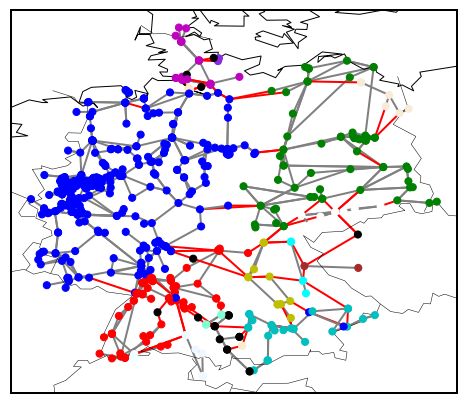
2

mental Material [35], section II, for details.                                              The planning stage concerns how the operational line
                                                                                            limits f̄ are set. For this, we solve (2) without (3), yielding
                                         3.0                                                                                          (pl)    Pn
                                                 Fitted (xmin, α), city sizes               the uniform (across cities) solution gj = n1 i=1 Xi for
                                         2.6
                                                 Fitted (xmin, α), blackout sizes
                                         2.2
                                                                                            all j ≥ 1, and f (pl) = −VX (see [35], section IV). Then,
                                         1.8
                                                                                            the operational line limits f̄ are set as

                                     α
                                                                                                            (pl)
                                         1.4
                                                                                                   f¯` = λ|f` | = λ|(VX)` |,          ` = 1, ..., m,   (4)
                                         1.0

                                         0.6                                                where λ ∈ (0, 1] is a safety tuning parameter, referred to
                                         0.2 3                                              as loading factor. In the operational stage, we solve (2)
                                           10        104          105           106
                                                              xmin                          subject to (3), yielding a different solution g(op) which
                                                                                            is not uniform due to the constraint (3). Eq. (4) implies
Figure 1: Left: Pareto tail behavior of US city [25] and blackout                           that line flows can have a heavy tail, which is consistent
     sizes [36] in the region x > xmin . Estimates are based on                             with impedance data [39]. This property is essential, as
PLFIT [25]. Points depict the empirical complementary cumulative                            it allows to create a subnetwork in which the mismatch
 distribution function (CCDF); Solid line depicts the CCDF of a
Pareto distribution with parameters α, xmin . Right: Hill estimator                         between supply and demand is heavy-tailed.
  xmin → α(xmin ), also known as the Hill plot [35]. The PLFIT                                 This mismatch is established in the emergency stage,
estimates for city sizes (blue dot) and blackout sizes (red dot) lie                        which is described next. We focus on cascades initiated by
within a relatively flat region of the graph, providing support for
                                                                                            a single line failure, sampled uniformly across all lines. A
                            the Pareto fit.
                                                                                            line failure changes the topology of the grid and causes a
                                                                                            global redistribution of network flows according to power
   In what follows, we make our claim rigorous by intro-
                                                                                            flow physics. Consecutive failures occur whenever there
ducing a new mathematical framework that captures the
                                                                                            are one or more lines for which the redistributed power
salient characteristics of actual power system dynamics [1]
                                                                                            flow exceeds its emergency line limit F` = f¯` /λ. Failures
and sheds light on the connection between blackout and
                                                                                            are assumed to occur subsequently, and take place at the
city sizes. For a full account, see [35], section IV.
                                                                                            line where the relative exceedance is largest. Whenever
   We consider a network with n nodes and m lines. Node i
                                                                                            line failures create additional islands, we proportionally
represents a city with Xi inhabitants. We consider a static
                                                                                            lower either generation or demand at all nodes to restore
setting where each inhabitant demands one unit of energy.
                                                                                            power balance. The cascade continues within each island
We assume that the Xi ’s are independent and identically
                                                                                            until none of the remaining emergency line limits are
distributed Pareto random variables with P (X > x) ≈
                                                                                            exceeded anymore.
Kx−α for constants K, α > 0. For convenience, we label                                         Our formulation may be extended to handle multiple
the nodes such that X1 represents the largest city.                                         initial failures, correlated city sizes, generator failures,
   For the electricity line flows, we adopt a linear DC power                               simultaneous failures, generation limits, other strictly
flow model. This model approximates the more involved                                       convex supply cost functions, and other load-shedding
AC power flow equations, is widely used in high-voltage                                     mechanisms. Such variations would affect the value of
transmission system analysis [37], and accurately de-                                       the pre-factor C, but not the exponent α: the tail of the
                                                                                            blackout distribution is dominated by the scenario where
scribed the evolution of the 2011 San Diego blackout [38].
                                                                                            there is a single city that has a large power demand, while
Specifically, if g = (g1 , ..., gn ) and X = (X1 , . . . , Xn ) rep-                        the demand of the other cities is negligible. A formal
resent the power generation and demand at each city, then                                   version of this statement is that, for sufficiently small ,
the line flows f = (f1 , ..., fm ) are given by f = V(g − X),
                                                                                             P (S > x) = P (S > x; X1 > x, Xi ≤ x, i ≥ 2) + o(x−α ). (5)
where the matrix V ∈ Rm×n is determined by the network
topology and the line reactances.                                                             This is a mathematical description of the aforemen-
   Our framework consists of three stages called planning,                                  tioned principle of a single big jump. After a normal-
operational and emergency. The first two stages determine                                   ization argument, it suffices to consider the case where
the actual line limits and line flows. We employ the widely                                 X1 = y > 0 and Xj = 0 for j ≥ 2. Then, the solution of
used Direct Current Optimal Power Flow (DC-OPF) for-                                        the operational DC-OPF can be computed in closed form:
mulation with quadratic supply cost functions [1]:                                            (op)                             (op)
                                                                                            g1 = (1 − λ(n − 1)/n)y and gj           = (λ/n)y for j ≥ 2
                               n                                                            (see [35], Lemma IV.2). Let A1 be the set of nodes that
                             1X 2
                      min         g                                                         represents the island containing the largest city, after the
                       g     2 i=1 i                                                        cascade has stopped. The islands that do not contain the
                                                                                      (2)
                             n
                             X             n
                                           X                                                largest city must lower their generation to zero after a dis-
                      s.t.         gi =          Xi ,                                       connection, and hence immediately turn stable. Iterating,
                             i=1           i=1                                              the blackout size in component A1 is given by
subject to the reliability constraint                                                               X                X                  n − |A1 |
                                                                                               S=       (Xi − gi ) =     (gj − Xj ) = λ           y. (6)
                     − f̄ ≤ V(g − X) ≤ f̄ .                                           (3)                                                  n
                                                                                                   i∈A1              j6∈A1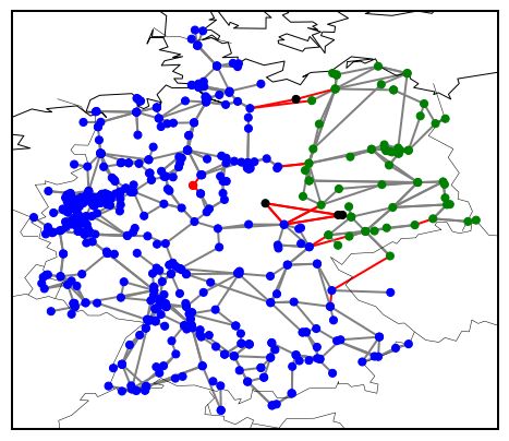
3
Figure 2: Cascade in a 6-node network with X1 = 1, Xj = 0 for j ≥ 2, λ > 3/4. The four lower and upper line flows are λ/24 and 5λ/24,
respectively, with corresponding emergency limits 1/24 and 5/24. The failure of an upper line causes the load on the adjacent lower line to
surge to λ/6 > 1/24, causing this line to trip (Stage 2). This cutoff leads to the load on the three remaining lower lines to surge to λ/18,
causing them to trip as well (Stage 3). After isolating node 2 and 6, the cascade ends with |A1 | = 4 and a total load shed of 2λ/6 (Stage 4).
Integrating over realizations of X1 = y, y ≥ x, and using long as these limits are a non-negligible fraction of the
the property of Pareto tails P( max(X1 , . . . , Xn ) > x) ≈ total demand.
nP(X > x) ≈ nKx−α [33], we find that (1) holds with To illustrate the sensitivity of our result with respect
n−1
X to the chosen power flow model, we partially extend our
C = nK P (|A1 | = j) λα (1 − j/n)α ∈ [0, ∞). (7) framework to the AC power flow model. We tested its
j=1 effect on multiple network topologies, and as illustrated
The most delicate step, for which [35], section IV.D pro- in Fig. 3a, we conclude that city size tails still drive the
vides a rigorous proof, is to show that the cascade sequence blackout size tail even when the DC assumption is violated.
does not change when performing the normalization ar- Intuitively, the chosen power flow model determines the
gument in the limit x → ∞, which is non trivial due to redistribution of flow after failures, and thus the cascade
continuity issues. sequence. This effect is captured in the prefactor, but
In [35], section IV, we show that the pre-factor C in (7) does not destroy the Pareto-tailed consequence in the
is discontinuous at a discrete set of values of λ. At such blackout size.
points, the number of possible scenarios leading to a large An important remark is that our mathematical frame-
blackout is increasing, and/or |A1 | is decreasing in λ. We work relies on the city sizes to be random variables. Nat-
illustrate this in Fig. 2, which also shows how the principle urally, city sizes are essentially fixed. The remaining
of a single big jump (5), which links the total blackout size source of randomness in our framework, namely the lo-
to the size of the largest city X1 , is realized by means of a cation of the first failure, can be interpreted as a mecha-
few load shedding events, each of which is a fixed fraction nism to bootstrap linear combinations of city sizes. It is
of X1 and corresponds to a network disconnection. well-known [33] that bootstrap methods cannot recover
Our analysis illustrates how heavy-tailed city sizes cause heavy-tailed behavior if the data set is small. In order to
heavy-tailed blackout sizes. Our modeling choices allow recover a Pareto tail, the frozen network therefore needs
for a precise exploration of the cascade sequence, and to be sufficiently large, e.g. 104 nodes. To illustrate this,
inherently, an explicit formula for the blackout size tail. Fig. 3b shows simulation results for the SynGrid model, a
However, we emphasize that the essential elements that random graph model designed to generate realistic power
lead to heavy-tailed blackout sizes are that both the grid topologies [39]. Finally, Fig. 3c reveals that Pareto-
demands and the line limits are heavy-tailed. The small tailed city sizes is a crucial assumption in order to recover
nodes together generate a non-negligible fraction of the the same scale-free behavior for blackout sizes, as light-
demand of the large node. When the power grid satisfies tailed city sizes do not lead to heavy-tailed blackout sizes.
these properties, then (5) continues to hold, leading to a Additional supporting experiments are reported in [35],
heavy-tailed mismatch whenever there is a disconnection. section VI.
We illustrate this numerically by studying the effect of We next present experimental results using the Sci-
relaxing several assumptions in our framework. GRID network [40, 41], a model of the German trans-
The choice of a quadratic cost function in the DC-OPF mission grid that includes generation limits and relaxes
ensures that it is most efficient to divide the power gen- several assumptions. We simulate blackout realizations
eration as equally as possible among the cities, causing by considering one year’s worth of hourly snapshots. For
all cities to generate a non-negligible fraction of the total each snapshot, we solve the operational DC-OPF and
demand. Other strictly convex increasing cost functions remove one line uniformly at random, initiating a cascade.
would lead to a similar effect. Moreover, our result is To assign city sizes to nodes, we have cities correspond to
robust to piecewise linear cost functions (see [35], Sec- German districts, and we assign a fraction of the popula-
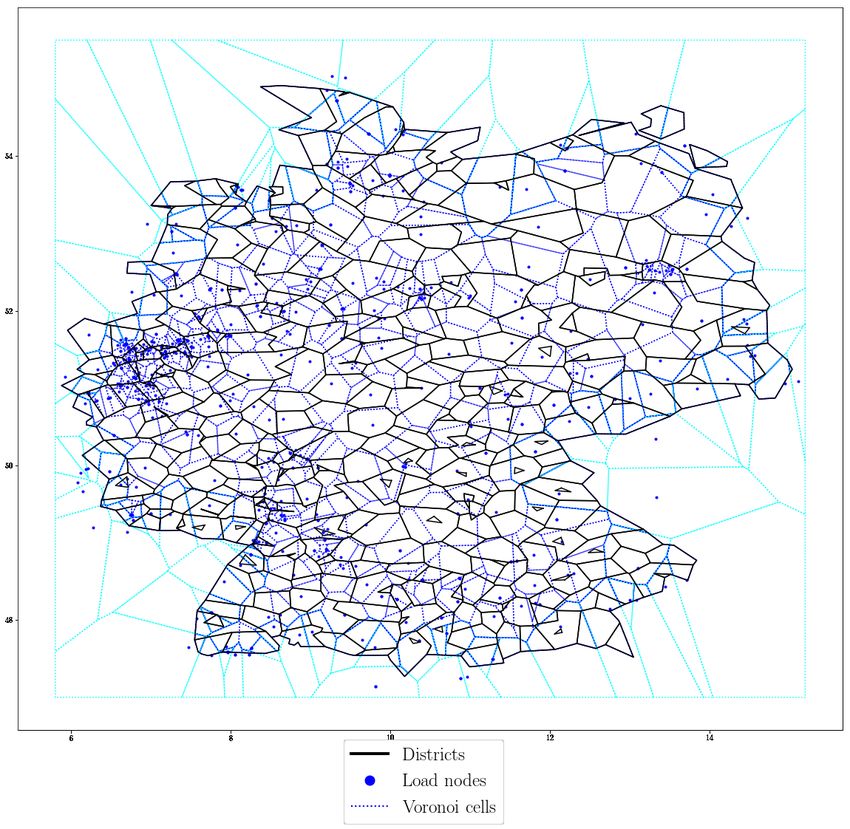
tion VI.C), and to the inclusion of generation limits, as tion of each district to specific nodes based on a Voronoi4
8
3.0
7
Customers Affected (×106 )
Customers Affected (×107 )
6 2.5
5 2.0
4
1.5
3
1.0
2
0.5
1
0 0.0
0 1 2 3 4 5 6 7 0 2 4 6 8 10 12
Cascade Stage Cascade Stage
(a) IEEE 39-bus (b) SynGrid model, (c) SynGrid model,
network, AC power n = 104 , frozen city n = 104 , frozen city
flow model. sizes. sizes sampled from
uniform distribution.
Figure 3: Pareto tail behavior of simulated blackout sizes using
the described cascade model with relaxed assumptions, for different
topologies and loading factor λ = 0.9. City sizes are sampled from
a Pareto distribution with tail index α(city) = 1.37 in (a,b), and
from a uniform distribution with the same mean in (c). Top:
points depict the empirical CCDF, dashed line depicts the CCDF
of a Pareto distribution with parameters α, xmin , estimated via Figure 4: Dissection of a massive blackout in the SciGRID
PLFIT [25]. Bottom: Hill plots. Red line corresponds to the tail network for loading factors λ = 0.7 (left) and λ = 0.9 (right) in
index α(city) . A good fit is achieved when the PLFIT estimate terms of the cumulative number of affected customers at each stage
(blue dot) lies in a flat region closely tracing the red line. of the cascade, as displayed in the top charts with the selected
stage colored red. The corresponding islanded components are
visualized with different colors in the bottom pictures.
tessellation procedure. In this way, we account for the
feature that a single city can encompass multiple nodes in
a network. For more details, we refer to [35], section VII. decrease in the likelihood of big blackouts. Consequently,
The German SciGRID network has a relatively small it is questionable whether network upgrades, as consid-
number of nodes (less than 600), and city sizes are frozen. ered in [19, 42], are the most effective way to mitigate
Therefore, we do not recover Pareto-tailed blackout sizes. the consequences of big blackouts.
However, uniformly across different loading factors λ, we Instead, it may be more effective to invest in responsive
found that the preponderance of blackouts involves just a measures that enable consumers to react to big blackouts.
single load shedding event due to a network disconnection. It is shown in [20] that durations of blackouts have a tail
For a moderate loading factor λ = 0.7, nearly 98% of which is decreasing much faster than (1). At the same
blackouts only involve a single disconnection. Even for a time, production facilities often lack redundancy - even
high loading factor λ = 0.9, 90% of the blackouts involve short blackouts can lead to huge costs, suggesting that
a single disconnection, and the fraction of blackouts with the costs associated to a blackout are concave up to a
four or more disconnections is below 4%. Fig. 4 depicts certain duration. Therefore, if the goal is to minimize
the largest observed blackout, for different values of λ. the negative effects of a big blackout, it may be far more
Even in this massive blackouts, the bulk of the total load effective to invest in solutions (such as local generation
shed is the result of a few load shedding events. These and storage) that aim at surviving a blackout of a specific
observations are typical properties that follow from our duration. This is consistent with recent studies on the
framework (see Fig. 2), and sharply contrast the branching importance of resilient city design [43].
process approximations where many small jumps take Finally, our framework and insights suggest new
place. ways of approaching scale-free phenomena in other
Using data analysis, probabilistic analysis, and sim- transportation networks, such as highway traffic jams [44].
ulations, we have illustrated how extreme variations in While transport network topologies are not scale-free,
city sizes can cause the scale-free nature of blackouts. they may still exhibit scale-free behavior, caused by the
Our explanation and refinement (7) of the scaling law (1) scale-free nature of nodal sizes.
show that specific details such as network characteristics
only appear in the pre-factor (7). The main parameter α, Acknowledgements. We thank Sem Borst for useful
which determines how fast the probability of a big black- discussions, and the Isaac Newton Institute for support
out vanishes as its size grows, is completely determined and hospitality during the program “Mathematics of En-
by the city size distribution. Decreasing the constant (7) ergy Systems”. The grants NWO 639.033.413 , NWO
by performing network upgrades (which in our framework 024.002.003 and EPSRC EP/R014604/1 provided finan-
is equivalent to decreasing λ) would only lead to a modest cial support.5
8, 165 (1980).
[32] M. Batty, Science 319, 769 (2008).
[33] S. I. Resnick, Heavy-tail phenomena, Springer Series in
[1] D. Bienstock, Electrical transmission system cascades and Operations Research and Financial Engineering (Springer,
vulnerability - an operations research viewpoint, MOS- New York, 2007) pp. xx+404.
SIAM Series on Optimization, Vol. 22 (SIAM, 2016). [34] J. Nair, A. Wierman, and B. Zwart, The Fundamentals
[2] F. Dörfler, M. Chertkov, and F. Bullo, Proceedings of Heavy-tails: Properties, Emergence, and Identification.
of the National Academy of Sciences 110, 2005 (2013), [35] “See Supplemental Material for the extended mathemat-
https://www.pnas.org/content/110/6/2005.full.pdf. ical framework and the details on the statistical data
[3] J. W. Simpson-Porco, F. Dörfler, and F. Bullo, Nature analysis and simulations, which includes refs. [45-58],”.
Communications 7 (2016), 10.1038/ncomms10790. [36] US Department of Energy, “Electric emergency inci-
[4] B. Schäfer, D. Witthaut, M. Timme, and V. Latora, dent and disturbance report (form OE-417),” https:
Nature communications 9, 1975 (2018). //www.oe.netl.doe.gov/OE417_annual_summary.aspx,
[5] T. Nesti, A. Zocca, and B. Zwart, Phys. Rev. Lett. 120, [Online; accessed November 2018].
258301 (2018). [37] K. Purchala, L. Meeus, D. Van Dommelen, and R. Bel-
[6] D. Watts, Proceedings of the National Academy of Sci- mans, in IEEE Power Engineering Society General Meet-
ences of the United States of America 99, 5766 (2002). ing (IEEE, 2005) pp. 2457–2462.
[7] F. Morone and H. A. Makse, Nature 524, 65 (2015). [38] A. Bernstein, D. Bienstock, D. Hay, M. Uzunoglu, and
[8] J. Hindes and I. B. Schwartz, Phys. Rev. Lett. 117, 028302 G. Zussman, in IEEE INFOCOM 2014 - IEEE Conference
(2016). on Computer Communications (2014) pp. 2634–2642.
[9] R. Pastor-Satorras and A. Vespignani, Phys. Rev. Lett. , [39] Z. Wang, A. Scaglione, and R. J. Thomas, IEEE Trans-
3200 (2001). actions on Smart Grid 1, 28 (2010).
[10] P. D. H. Hines, I. Dobson, and P. Rezaei, IEEE Transac- [40] C. Matke, W. Medjroubi, and D. Kleinhans, Mathematics
tions on Power Systems 32, 958 (2017). and Physics of Multilayer Complex Networks (2015).
[11] A. E. Motter, Phys. Rev. Lett. 93, 098701 (2004). [41] T. Brown, J. Hörsch, and D. Schlachtberger, Journal of
[12] D. Witthaut, M. Rohden, X. Zhang, S. Hallerberg, and Open Research Software 6 (2018).
M. Timme, Phys. Rev. Lett. 116, 138701 (2016). [42] Y. Yang, T. Nishikawa, and A. E. Motter, Science 358,
[13] Y. Yang and A. E. Motter, Phys. Rev. Lett. 119, 248302 eaan3184 (2017).
(2017). [43] X. Bai, Nature 559 (2018).
[14] B. Schäfer, C. Beck, K. Aihara, D. Witthaut, and [44] L. Zhang, G. Zeng, D. Li, H.-J. Huang, H. E.
M. Timme, Nature Energy 3, 119 (2018). Stanley, and S. Havlin, Proceedings of the Na-
[15] D. Witthaut and M. Timme, Physical Review E 92, tional Academy of Sciences 116, 8673 (2019),
032809 (2015). https://www.pnas.org/content/116/18/8673.full.pdf.
[16] P. Crucitti, V. Latora, and M. Marchiori, Physical Review [45] B. M. Hill, Ann. Statist. 3, 1163 (1975).
E 69, 045104 (2004). [46] P. v. Mieghem, Graph Spectra for Complex Networks
[17] L. Huang, L. Yang, and K. Yang, Phys. Rev. E 73, 036102 (Cambridge University Press, 2010).
(2006). [47] P. Van Mieghem, K. Devriendt, and H. Cetinay, Phys.
[18] B. A. Carreras, V. E. Lynch, I. Dobson, and D. E. New- Rev. E 96, 032311 (2017).
man, Chaos: An Interdisciplinary Journal of Nonlinear [48] P. TøNdel, T. A. Johansen, and A. Bemporad, Automat-
Science 14, 643 (2004). ica 39, 489 (2003).
[19] I. Dobson, B. A. Carreras, V. E. Lynch, and [49] D. J. Watts and S. H. Strogatz, nature 393, 440 (1998).
D. E. Newman, Chaos: An Interdisciplinary [50] Z. Wang, H. Sadeghian, S. H. Elyas, R. D. Zimmerman,
Journal of Nonlinear Science 17, 026103 (2007), E. Schweitzer, and A. Scaglione, (2018).
https://doi.org/10.1063/1.2737822. [51] R. D. Zimmerman, C. E. Murillo-Sánchez, and R. J.
[20] P. Hines, K. Balasubramaniam, and E. C. Sanchez, IEEE Thomas, Power Systems, IEEE Transactions on 26, 12
Potentials 28, 24 (2009). (2011).
[21] B. A. Carreras, D. E. Newman, and I. Dobson, IEEE [52] D. K. Molzahn and I. A. Hiskens, A Survey of Relaxations
Transactions on Power Systems 31, 4406 (2016). and Approximations of the Power Flow Equations (2019).
[22] A.-L. Barabási and R. Albert, Science 286, 509 (1999). [53] T. Brown, https://pypsa.org/examples/
[23] B. Suki, A.-L. Barabási, Z. Hantos, F. Peták, and H. E. scigrid-lopf-then-pf.html (2017).
Stanley, Nature 368, 615 (1994). [54] World Population Review, http://
[24] A.-L. Barabási, Nature 435, 207 (2005). worldpopulationreview.com/countries/
[25] A. Clauset, C. R. Shalizi, and M. E. Newman, SIAM germany-population/cities/, [Online; accessed
review 51, 661 (2009). on October 2018].
[26] H. A. Simon, Biometrika 42, 425 (1955). [55] Eurostat, http://appsso.eurostat.ec.europa.eu/nui/
[27] P. Bak, C. Tang, and K. Wiesenfeld, Phys. Rev. A 38, show.do?dataset=nama_10r_3popgdp, [Online; accessed
364 (1988). on October 2018].
[28] K. Sun, Y. Hou, W. Sun, and J. Qi, Power system control [56] Eurostat, “Nuts rg 60m 2013.shp,” https://ec.europa.
under cascading failures: understanding, mitigation, and eu/eurostat/web/gisco/geodata/reference-data/
system restoration (Wiley-Blackwell, 2018). administrative-units-statistical-units/nuts#
[29] J. Kim and I. Dobson, IEEE Transactions on Reliability nuts13, [Online; accessed on October 2018].
59, 691 (2010). [57] Data Packaged Core Datasets,
[30] G. K. Zipf, Social Forces 28, 340 (1950). “Nuts rg 60m 2013.shp,” https://github.com/
[31] K. T. Rosen and M. Resnick, Journal of Urban Economics datasets/geo-nuts-administrative-boundaries/6
blob/master/data/NUTS_2013_60M_SH/data/NUTS_RG_
60M_2013.shp, [Online; accessed on October 2018].
[58] T. Brown, https://pypsa.org/examples/add_load_
gen_trafos_to_scigrid.html (2017), [Online; accessed
on December 2017].7
Supplemental Material for:
Emergence of scale-free blackout sizes in power grids
BACKGROUND ON PARETO DISTRIBUTION per the 2000 US census, are available in [25]. The data for
AND PARAMETER ESTIMATION US blackouts are extracted from the Electric Disturbance
Events Annual Summaries, Form OE-417 [36] of the US
A Pareto-distributed random variable X with minimum Department of Energy, which includes information on the
value xmin > 0 and tail exponent α > 0 is described by its date, area of interest and number of customers affected
complementary cumulative distribution function (CCDF) by outage events. Here, the size of a blackout is defined
F̄ (x) as the number of customers affected by it. The dataset
x −α covers the period 2002-2018.
F̄ (x) = P(X > x) = , x ≥ xmin . (8) Each record, or row, of the OE-417 dataset, contains
xmin
information such as the date, area of interest and the
The expected value of X is equal to (αxmin )/(α − 1) if number of customers affected in a single outage event.
α > 1, and ∞ otherwise. The presence of missing or noisy records in the dataset
In order to analyze the power law behavior of city and requires the following pre-processing actions: i) records
blackout sizes, we use the PLFIT method introduced for which the “Number of customers affected” entry is un-
in [25] to fit a Pareto distribution to a given empirical known are removed; ii) records for which the “Number of
dataset {xi }Ni=1 . The PLFIT method is based on a com- customers affected” consists of two or more values, corre-
bination of the Hill estimator to find the tail exponent sponding to different US states, are modified by replacing
α, and on the Kolmogorov-Smirnov statistic to find xmin , the multiple values with their sum; iii) records for which
as outlined below. For each possible choice of xmin , the the “Number of customers affected” entry is not purely
best-fitting tail index α is found via the Hill estimator [45] numeric are removed. The only two exceptions to iii)
h X xi i−1 are when both the âĂIJcumulativeâĂİ and âĂIJpeakâĂİ
α̂(xmin ) = n ln . number of customers affected are reported (in which case
xmin
xi ≥xmin
only the âĂIJcumulativeâĂİ values is retained), and when
Then, the KS goodness-of-fit statistic D(xmin ) = the number of customers affected is described by a range
maxx≥xmin |S(x) − P (x)| is calculated, where S(x) is the of values (in which case the midpoint value is retained).
empirical Cumulative Distribution Function (CDF) of the Table I reports the PLFIT estimated parameters, the
data and P (x) is the CDF of the Pareto distribution with corresponding standard deviations (calculated using the
parameters xmin and α̂(xmin ). Finally, the estimated x̂min nonparametric bootstrap method in [25]), as well as the
is the one that minimizes D over all possible choices of KS p-values, which indicate a good fit. The results for
xmin . Uncertainty in the estimated tail exponent α̂(x̂min ) the α-estimates (city sizes: 1.37 ± 0.06; blackout sizes:
and lower bound x̂min is quantified via the nonparametric 1.31 ± 0.08 ) corroborate the claim that the scale-free
bootstrap method described in [25]. Finally, a goodness- behavior of blackout sizes is inherited from the power law
of-fit test based on the KS statistic is used to generate distribution for city sizes.
a p-value that quantifies the plausibility of the power
Fig. 5a reports the CCDF and the PLFIT results, and
law hypothesis. The authors in [25] suggest to use the
Fig. 5b the corresponding Hill plots. We observe that the
following (conservative) choice: the power law is ruled out
estimated parameters lie in the flat portion of the Hill
if p ≤ 0.1.
plots.
We remark that any automatic procedure for the es-
timation of the parameter xmin is imperfect and should
be paired with additional, case-by-case analysis. For in-
stance, it is not known whether the PLFIT estimator is
POWER FLOW
consistent. In this paper, we always couple the PLFIT
procedure with the manual observations of the Hill plot,
i.e. the graph of the mapping xmin → α̂(xmin ), and report We model the power grid as a connected graph G =
whether the PLFIT results are consistent with the visual G(N , L), where the set of nodes N represents the n buses
analysis of this plot, i.e. whether x̂min lies within a region in the system, and the set of edges L corresponds to the
where the values of α are relatively stable. m transmission lines. Let g, d ∈ Rn represent the nodal
generation and load vectors, respectively, and p = g − d
be the net power injections vector. We make use of
HISTORICAL DATA ANALYSIS the DC approximation, which is commonly used in high-
voltage transmission system analysis [37], to model the
In this section, we analyze the scale-free behavior of US relationship between active power injections p and active
city and blackouts sizes. The data for US city sizes, as line power flows f ∈ Rm , which is given by the linear8
Dataset N ntail α̂(x̂min ) x̂min KS p-value
US city sizes, 2000 Census (×103 ) 19447 580 1.37 ± 0.08 52.5 ± 11.6 0.76
US blackout sizes, form OE-417 (×103 ) 1341 448 1.31 ± 0.08 140 ± 31.3 0.32
Table I: PLFIT statistics for US city and blackout sizes. ntail is the number of data points xi ≥ x̂min . Standard deviations
obtained via nonparametric bootstrap with 1000 repetitions.
mapping
f = V(g − d). (9)
The matrix V ∈ Rm×n is known as the Power Transfer
Distribution Factors (PTDF) matrix and is constructed
as outlined below.
PTDF matrix
Choosing an arbitrary but fixed orientation of the trans-
mission lines, the network structure is described by the
edge-vertex incidence matrix C ∈ Rm×n defined as
1
if ` = (i, j),
(a) Pareto tail behavior of US city and blackout sizes in the C`,i = −1 if ` = (j, i),
region x > xmin . Estimates for α and xmin , along with
0 otherwise.
standard deviations, are based on PLFIT [25]. Points
represent the empirical complementary cumulative
distribution function (CCDF); Solid line represents the Denote by β` > 0 the weight of edge ` ∈ L, corre-
CCDF of a Pareto distribution with parameters α, xmin . sponding to the susceptance of that transmission line.
Note that β` = x−1 ` , where x` is the reactance of line
3.0 `. Denote by B the m × m diagonal matrix defined as
Fitted (xmin, α), city sizes B = diag(β1 , . . . , βm ). The network topology and weights
2.6
Fitted (xmin, α), blackout sizes are simultaneously encoded in the weighted Laplacian ma-
2.2 trix of the graph G, defined as L = C> BC or entry-wise
as
1.8 (
−βi,j if i 6= j,
α
Li,j = P
1.4
k6=j βi,k if i = j.
1.0 All the rows of L sum up to zero and thus the matrix L
is singular.
0.6 According to the DC approximation, the relation be-
0.2 3
tween any zero-sum vector of power injections p ∈ Rn and
10 104 105 106 the phase angles θ ∈ Rn can be written in matrix form
xmin as p = Lθ. Defining L+ ∈ Rn×n as the Moore-Penrose
pseudo-inverse of L, we can rewrite this as
(b) Visualization of the estimated α, obtained by only taking
into consideration values in the region x > xmin , as a function θ = L+ p. (10)
of xmin . The PLFIT-estimated xmin for city sizes (blue dot)
and blackout sizes (red dot) lie within a region where the
The line power flows f are related to the phase angles θ
values of α are relatively stable, substantiating the results of via the linear relation f = BCθ. In view of (10), the line
the PLFIT procedure. power flows f can be written as a linear transformation
of the power injections p, i.e.
Figure 5: Pareto tail behavior of US city and blackout sizes.
f = Vp, (11)
where V := BCL+ is the PTDF matrix.
The following lemma is based on a well-known result
in graph theory (see, for example, [46]).9
Lemma .1 If G is a connected graph, rk (V) = rk (C) =
rk (L) = rk (L+ ) = n − 1, and the null space of V is the n
X
one-dimensional subspace generated by e = (1, . . . , 1) ∈ minn Ci (gi ) (12)
g∈R
Rn , i.e. i=1
Xn n
X
Ker (V) = Ker (C) = Ker (L) = Ker (L+ ) =< e > . s.t. gi = di , (13)
i=1 i=1
g i ≤ gi ≤ ḡi , i ∈ N, (14)
The following lemmas are technical results which will
be needed in Section . −f¯` ≤ V` (g − d) ≤ f¯` , ` ∈ L, (15)
Ci (·) : R → R denotes the cost function of generation
Lemma .2 Changing the orientation of a subset of lines at node i, g, ḡ ∈ Rn denote, respectively, the vector of
L0 ⊂ L has the effect of swapping the sign of the cor- nodal minimum and maximum generation capacities, and
responding rows of the PTDF matrix V. In particular, f̄ ∈ Rm denotes the vector of line limits. We assume that
it is always possible to choose the orientation such that Ci (·) is an increasing quadratic function. Specifically,
Ve1 ≥ 0. we assume Ci (gi ) = gi2 /2, i = 1, ..., n. For the purpose
of this work, we do not consider generator limits, i.e.
Proof. Changing the orientation of a line from lk = g i = −∞, ḡi = ∞, i = 1, ..., n.
(i, j) to ˜lk = (j, i), by definition, amounts to swapping
the sign of the k-th row of matrix C, yielding a modified
Power flow redistribution
matrix C̃ = I(k) C, where I(k) is a diagonal matrix with
(k) (k)
Iii = 1 if i 6= k and Ikk = −1. Since L̃ = C̃> C̃ =
> (k) (k) > In the event of the failure of a subset of transmission
C I I C = C C = L, the matrices L and L+ are not
lines L0 ⊂ L, and provided that the power injections re-
affected by the change. As a consequence, the modified
main unchanged, the power flows will redistribute among
PTDF matrix V = BC̃L+ = I(k) V differs from V only
the remaining lines according to power flow physics, pro-
by the swapped signs on the k-th row. e = (N , L \ L0 ) remained
vided that the altered graph G
connected. The way the power flows redistribute is gov-
Lemma .3 Let G be assigned the orientation such erned by the new PTDF matrix V, e which can be con-
that the set of edges incident to node 1 is L1 = structed analogously to V, mapping the (unchanged)
{(1, j) | j is adjacent to 1}, i.e. C`,1 = 1 = −C`,j for all power injections to the new power flows. We assume that
` = (1, j) ∈ L1 . Then, V`,1 ≥ 0 for every ` ∈ L1 . The the redistribution occurs instantaneously, without any
converse is also true. transient effects.
As an illustration, we show how the redistributed power
flows can be calculated in the special case of an isolated
Proof. First, note that largest element in each row of L+ failure L0 = {`}. In this case, it is enough to calculate the
is its diagonal entry (Corollary 1 in [47]), i.e. L+ +
1,1 −L1,j ≥ vector φ(`) ∈ Rm−1 of redistribution coefficients, known
0 for every ` = (1, j) ∈ L1 . For any line ` = (1, j) ∈ L1 , (`)
as line outage distribution factors. The quantity φj takes
we have V`,1 = (CL+ )`,1 = C`,1 L+ +
1,1 + C`,j L1,j , where
(`)
values in [−1, 1], and |φj | represents the percentage of
C`,1 = −C`,j = ±1 depending on the orientation of line `. power flowing in line ` that is redirected to line j after the
Thus, V`,1 ≥ 0 if and only if C`,1 = 1 = −C`,j . failure of the former. In particular, the new power flow
configuration after the failure of line ` = (i, j), denoted
by f (`) ∈ Rm−1 , is given by
Optimal Power Flow (`) (`) (`)
fk = fk + f` φk , ∀` 6= k, (16)
where, for k = (a, b) and ` = (i, j), the coefficient φk,` ∈ R
The Optimal Power Flow (OPF) program is an opti-
can be computed as
mization problem that determines the generation sched-
ule minimizing the total system generation cost while Ra,j − Ra,i + Rb,i − Rb,j
φk,` = φ(i,j),(a,b) = β`−1 · , (17)
satisfying demand/supply balance and network physical 2(1 − x−1
i,j Ri,j )
constraints. In its full generality, the OPF is a nonlinear,
nonconvex optimization problem. For the purpose of this where Ri,j is the effective resistance between nodes i and
paper, we will focus on a tractable approximation based j, given by
on the DC power flow equations referred to as DC-OPF, Ri,j = (ei −ej )T L+ (ei −ej ) = (L+ )i,i +(L+ )j,j −2(L+ )i,j .
which can be formulated as the following optimization
problem: .10
CASCADING FAILURE MODEL Finally, in the emergency problem, we focus on the
failure process after an initial disturbance. We assume
In view of the DC-OPF, in order to obtain a funda- that the initial failure is caused by a single line failure,
mental understanding of the correlation between blackout chosen uniformly at random over all lines. We point out
sizes and city sizes using the DC approximation model, that our framework can be extended to multiple initial
we require a framework that adequately sets the power line failures, or adapted to deal with generator failures.
demand, the transmission line limits, generation limits, The initial failure may cause a cascading effect that leads
and the cost function for any fixed topology G = (N , L). to multiple line failures that disintegrate the network. A
In addition, we need to specify a mechanism that causes consecutive line failure occurs whenever there is at least
the initial line failure, as well as which lines possibly fail one line such that its emergency line limit is exceeded.
next after the power flow redistribution. For this purpose, That is, instead of considering the conservatively chosen
we consider a framework that consists of three problems: operational line limits f¯` , we take the line limits to be F` =
the planning problem, the operational problem, and the λ∗ f¯` for some constant λ∗ > 1. A canonical choice is λ∗ =
emergency problem. Next, we explain our framework in 1/λ. We assume that line failures occur subsequently, and
more detail, followed by listing some vital properties. occurs at the line where its relative exceedance is largest.
Whenever line failures cause the network to disconnect
in multiple islands, we assume that the energy balance is
Description of the framework restored by proportionally lowering either generation or
demand at all nodes. Naturally, this alters the line power
The planning problem refers to how the generation lim- flows. More specifically, before the initial disturbance
its, the line limits and power demand are determined with occurs, the network flows are given by V(g − X), where g
respect to the city sizes X1 , ..., Xn . We assume that each is the solution of the DC-OPF in the operational problem.
node represents a city with size Xi inhabitants. For ease After any line failure, we check whether this causes the
of presentation, we consider a framework with a static network to disconnect, and if so, we proportionally lower
setting where each inhabitant demands one unit of energy, the generation in one component and the demand in
i.e. di = Xi for every i = 1, ..., n. We assume that the the other component such that demand and generation
cost function is an increasing quadratic function and that are balanced in the two disconnected components. The
generator limits do not pose an effective constraint in the network flows are updated according to the laws of physics
DC-OPF. In other words, Ci (gi ) = gi2 /2, i = 1, ..., n, and in every component. That is, the removal of one or
g i = −∞, ḡi = ∞, i = 1, ..., n. The line limits are set as a more lines yields a modified matrix V e (see Section ), and
fraction of the absolute power flow in a setting where also possibly modified generation g̃ and demand d̃. The line
the line limits pose no effective constraint. More specifi- flows are given by V(g̃−
e d̃). This cascading failure process
cally, in the absence of any generator and transmission line continues until the line limits F` of all surviving lines are
limits, it is easy to sufficient to carry the power flows.
Pnsee that the solution of the DC-OPF
is g(planning) = n1 i=1 Xi e. The associated flow vector is This iterative process leads to a network having discon-
given by f (planning) = V(g(planning) − X) = −VX, where nected sets. We make the convention that A1 is the set
we used that Vg∗ = 0 (Lemma .1). For a safety loading of nodes that contains the city with the largest demand
factor λ ∈ [0, 1], referred as loading factor in the rest, the after the cascade has taken place. We point out that the
operational line limits are set as set A1 is random, and in particular, A1 = {1, ..., n} if the
cascade stops without causing network disconnections.
f̄j = λ |(VX)j |, j = 1, ..., m. (18) Whenever the network disintegrates in multiple com-
ponents, we alter the generation and demand to restore
In the operational problem, we solve the DC-OPF for the power balance in every component. We approximate
an increasing quadratic cost function and line limits as the total of load that is shed or equivalently, the number
in (18) to obtain the generation vector g. That is, we of customers affected by the blackout, by the mismatch
solve between generation and demand in the component con-
n
X taining the city with highest power demand, defined as
minn gi2 /2 (19)
g∈R
i=1 X
Xn n
X S= (Xi − gi ) . (22)
s.t. gi = Xi , (20) i∈A1
i=1 i=1
VX − λ |VX| ≤ Vg ≤VX + λ |VX| , (21) Due to properties of the Pareto distribution, this turns
out to be a good approximation as it yields exactly the
where |VX| denotes the vector with elements (|VX|)j = same limiting behavior. We study this notion in more
|(VX)j |, j = 1, ..., m. detail in the next sections.11
Principle of a single city with large demand Closed-form solution for the operational OPF in the
case d = e1 .
A vital property in our framework is that the only likely
way to have a large blackout is when there is a single Note that without loss of generality, we can always
city that has a large power demand. To formalize this normalize our framework by dividing all parameters (e.g.
notion, write d1 = max{d1 , ..., dn } with di , i = 1, ..., n generation, line limits, etc.) by the sum of all power
independent and identically Pareto distributed power demands. This yields an equivalent setting where the
demands. Note that for every > 0, total power demand equals one. In view of Lemma .4,
it is sensible to consider the special case where d = e1 .
That is, node 1, henceforth referred to as the sink node,
P (S > x) = has unit demand, while all other nodes have zero demand.
For this special case, a closed-form solution exists for the
n
! n
!
X X
P S > x; di < d1 + P S > x; di ≥ d1 . generation vector in the operational OPF.
i=2 i=2 First, we consider the planning problem. As stated in
It turns out that we can show that (in certain settings) the model description, in the absence of any generator
the first term on the right-hand side has a Pareto tail, and transmission line limits, the solution of the planning
and the second term is negligible. More specifically, the OPF is g∗ = n1 e, with associated flow vector f ∗ = V(g∗ −
following result can be shown. e1 ) = −Ve1 , where we used that Vg∗ = 0 (Lemma .1).
Therefore, the operational problem (12)-(15) reduces to
Lemma .4 Suppose di , i = 1, ..., n are independent and
n
identically Pareto distributed with tail exponent α > 0, X
and write d1 = max{d1 , ..., dn }. For every > 0, as minn gi2 /2 (24)
g∈R
i=1
x → ∞,
! s.t. e g = e> e1 = 1,
>
(25)
n
X
−2α
−λ|Ve1 | ≤ V(g − d) ≤ λ|Ve1 |, (26)
P S > x; di ≥ d1 = O x . (23)
i=2
which we will denote by P (λ). Lemma .5 shows that the
Proof. We observe that the total mismatch can never solution of P (λ) is of closed form.
exceed the sum of all demands, and hence
n
X Lemma .5 Let λ ∈ (0, 1). Let G be assigned the orien-
S≤ di ≤ nd1 . tation such that Ve1 ≥ 0. Then, the solution of P (λ) is
i=1 given by
Therefore, 1
g(λ) = λ e + (1 − λ)e1 ,
n
n
!
X
P S > x; di > di ≥ d1
i=2 i.e. g1 (λ) = 1 − λ n−1 1
n and gi (λ) = λ n for all i = 2, . . . , n.
The corresponding line flows are at capacity and are given
x d1
≤P d1 > ; di > for some i = 2, ..., n by f (λ) = −λVe1 .
n n
x
≤P di > 2 for some i = 2, ..., n
n Proof. First, we note that the selected orientation
on G implies that the set of edges incident to node 1 is
Write I(y) = |{i : di > y}|. Since for every η > 0, L1 = {(1, j) | j is adjacent to 1} (i.e. the edges in L1 exit
P (I(ηx) ≥ 2) = O x−2α
node 1), or, in terms of the edge-node incidence matrix
C, that C`,1 = 1 = −C`,j for all ` = (1, j) ∈ L1 . This is
as x → ∞, the result follows. proved in Lemma .3 in Section .
In other words, Lemma .4 implies that if for some > 0 Due to the chosen orientation, f̄ (λ) = λ |Ve1 | = λVe1
sufficiently small, and the line limit constraints in P (λ) can be rewritten as
n
!
X (1 − λ)Ve1 ≤ Vg ≤ (1 + λ)Ve1 .
P S > x; di < d1 ∼ Cx−α
i=2
The problem P (λ) is a strictly convex optimization prob-
holds for some constant C ∈ (0, ∞), then the only likely lem with linear equality and inequality constraints. There-
way to have a large blackout is when there is a single city fore, in order to show that g(λ) is the unique optimal
that has a large demand. solution, it is sufficient to show that it satisfies the KKT12
conditions for P (λ), which read amount of reduced power generation at node 1 (power
imbalance), which is given by
g + V> (µ+ − µ− ) + γe = 0, (27)
+ −
X λ λ(n − |A1 |)
µ ≥ 0, µ ≥ 0, , (28) S= = . (34)
n n
i6∈A1
µ+
l (Vg − (1 + λ)Ve1 )` = 0 ∀` ∈ L, (29)
µ− Naturally, the way the failure process cascades through
l (−Vg + (1 − λ)Ve1 )` = 0 ∀` ∈ L, (30)
> the network after the initial disturbance is highly depen-
e g = 1, (31) dent on the network topology. The redistribution of power
(1 − λ)Ve1 ≤ Vg ≤ (1 + λ)Ve1 , (32) flow takes place as described in Section , and we stress
that this is a deterministic process. In this special case,
where γ is the Lagrange multipliers for the equality con- the only sources of randomness come from the choice of
straint and µ+ , µ− ∈ Rm are the Lagrange multipliers the initial line failure, and possibly the choice of subse-
for the inequality constraints. quent line failure whenever the redistribution of power
Since Vg(λ) = (1 − λ)Ve1 and e> g(λ) = e> e1 = 1, flow causes the relative exceedance to be the same at
the candidate solution g(λ) clearly satisfies the feasibility multiple lines. Therefore, given a network topology and
conditions (31),(32) and the complementary slackness the line that initially fails, we can determine exactly how
condition (30). Moreover, condition (29) is satisfied if we the failure process propagates through the network.
choose µ+ = 0. It may be apparent from Lemma .4 that this special case
Using the facts that Vg(λ) = (1 − λ)Ve1 and where d = e1 describes some form of limiting behavior.
Ker(V) =< e >, pre-multiplying equation (27) by V That is, as Lemma .4 holds for every > 0, we observe
yields (1 − λ)e1 + V> µ ∈ Ker(V). This is equivalent to that the normalized demand vector d converges to the
(1 − λ) unit vector e1 as ↓ 0. Next, we show that for almost all
(1 − λ)e1 + V> µ = e, values of λ, for all demand vectors d for which d → e1
n
as ↓ 0, the order at which line failures occur converges
where in the last equality we used again the property that to the sequence of line failures as if the demand vector
Ve = 0. To conclude the proof, it remains to be shown would have been d = e1 .
that that there exist a nonnegative solution µ− ≥ 0 of
the matrix equation
Convergence of cascade sequence
V> (−µ− ) = (1 − λ)(e/n − e1 ). (33)
The operational OPF
We construct a non-negative solution µ− as follows:
1 >
( min g g (35)
− (1 − λ) l ∈ L1 g∈Rn 2
µ` := (1 − λ)eL1 = ,
0 l∈/ L1 , s.t. e> g = e> d, (36)
|V(g − d)| ≤ λ |Vd| , (37)
where eL1 is a m- dimensional vector containing ones in po-
sitions given by L1 , and 0 elsewhere. Invoking Lemma .3 is a strictly convex optimization problem, and since g =
we see that Ce1 = eL1 , yielding µ− = (1 − λ)Ce1 . Using λd̄e + (1 − λ)d is a feasible point, the feasible set of this
the definition of V = CL+ , L = C> C, and the property optimization problem is nonempty. Therefore, for each
L+ L = (I − J/n) (see [47]), we observe that Eq. (33) is demand vector d, there exists a unique optimal solution
indeed satisfied: g∗ (d).
If we view d as a parameter of the problem, then (35)-
V> µ− = −(1 − λ)V> µ− = −(1 − λ)V> Ce1 (37) is an instance of a multi-parametric quadratic pro-
= −(1 − λ)(L+ L)e1 = (1 − λ)(e/n − e1 ). gramming (mp-QP) problem with a strictly convex ob-
jective function, for which it is known that the optimal
Setting γ = −1/n completes the proof. solution g∗ (d) is a continuous function of the parameter
Finally, we solve the emergency problem. Observe that vector d (Theorem 1, [48]). This continuity property will
whenever there is a network disconnection, the component be used extensively in the rest of this section.
that does not contain node 1 has no power demand, and We assume in our framework that line failures occur
hence the generation at every node in that component is subsequently, i.e. a next line failure occurs at the line
reduced to zero. Evidently, no consecutive failures occur where the line limit is relatively most exceeded. Recall
in this component. On the other hand, the demand at that Fj denotes the emergency line limit of line j ∈ L,
node 1 is reduced by the number of nodes that disconnect and is given by (taking λ∗ = λ1 )
from this component times λ/n. Therefore, the total
amount of load that is shed is exactly equal to the total Fj = λ∗ λ|(Vd)j | = |(Vd)j |.13
(m)
We write fj as the flow on line j after the failure of the This assumption is for technical convenience, and we
first m − 1 lines and after the load/generation shedding stress that our results hold more generally. In particular,
(1) this assumption rules out certain network topologies with
took place, where we use the convention that fj denotes
the flow on line j when no initial disturbance has occurred some form of symmetry, but we can slightly adapt the
(m)
yet, and fj = 0 if line j has already failed before the framework to deal with these cases as well.
m-th step of the cascading failure process. The cascade is That is, suppose that |A(m) | > 1 for some m ∈ N
initiated by the random failure of line ` = `(1) . The m-th and the set A(m) consists only of lines that are indistin-
line to fail, for m ≥ 2, is given by guishable from one another (lines that are ‘symmetric’).
Since nodal demands are independent and identically dis-
n |f (m) | − Fj o n |f (m) | o tributed, this implies that each of these lines has an equal
(m) j j
` = arg max = arg max , probability of being the line that fails next. By the sym-
j∈A(m) Fj j∈A (m) F j
metry of the network topology, regardless of which line
(38) is chosen to fail next, the resulting networks after the
(m) cascade are indistinguishable. We illustrate this notion
where A(m) = {j : |fj | ≥ Fj } is the set of lines that for the 6-node example in the next section.
exceed the limit. To analyze the power imbalance in this framework, we
need to introduce some notation as well as formally define
Remark .6 Note that the line limits and line flows de-
the shedding rule and the redistribution of power flows.
pend on d and λ through the operational OPF, so that
the sequence of subsequent failure depends on d, λ, and Definition .8 (Uniform shedding rule) Let g(1) =
on the initial failure ` = `(1) . That is, g∗ , d(1) = d be the initial generation and demand vectors.
(m) (m) Assume that the removal of lines `(1) , . . . , `(m) , m ≥ 1, dis-
Fj = Fj (d), fj = fj (d, λ), A(m) = A(m) (`, λ, d), (m) (m) (m)
connects the network in components Gi = (Ni , Li ),
`(m) = `(m) (`, λ, d). i = 1, . . . , hm . Define the power imbalance in component
(m)
Gi as
For the sake of exposition, we do not write the dependency
on d, λ and `. YG (m) =
X (m)
(gk − dk ).
(m)
i
(m)
Let C = {`(1) , . . . , `(T ) } be a cascade sequence, where k∈Ni
(T )
` is the last failure before the cascade stops. Such a
In order to re-achieve power balance, generation and de-
sequence is uniquely determined by the first failure `(1)
mand in each component are modified iteratively according
and by the demand vector d and by λ, i.e. C = C(d, λ, `). (m)
In view of Lemma .4 and the normalization property, the to the following uniform shedding rule, for k ∈ Ni :
goal of this section is to show that if d → e1 , then the
Y (m)
!
G (m)
cascade sequence does not depend on d anymore, i.e.
1− P
i
(m) dk if YG (m) < 0
(m+1) (m) dl
dk = l∈N
i
i ,
C(d, λ, `) = C(e1 , λ, `) if d → e1 .
d
(m)
if YG (m) ≥ 0
k i
We observe that if |A(m) | = 0, no more line failures
occur. Technically, it is also possible that |A(m) | > 1 and
(m)
hence the subsequent line failure next needs to be chosen gk if YG (m) < 0
i
(m+1)
!
out of a set of multiple lines. We exclude the cases that gk = Y (m)
G (m)
1− gk if YG (m) ≥ 0
i
do not yield unique maximizers from our framework.
P (m)
gl
(m) i
l∈N
i
Assumption .7 For all lines j, the ratios between redis-
tributed flows and line limits Definition .9 (Power flow redistribution) Assume
that the removal of lines `(1) , . . . , `(m) , m ≥ 1, discon-
(m) (m) (m) (m)
|fj (e1 )| λ|(V(m) e1 )j | nects the network in components Gi = (Ni , Li ),
= i = 1, . . . , hm . Then, the line flows in component Gi
(m)
Fj (e1 ) |(Ve1 )j |
are given by
are all different for all m ≥ 2, where V(m) denotes the (m+1) (m+1) (m+1)
PTDF matrix for the remaining network after m − 1 fLi = V(m+1,Gi ) (gNi − dNi ),
failures have taken place. This assumption is needed to
ensure the uniqueness of the maximizer in (38). where V(m+1,Gi ) is the PTDF matrix for the subgraph
(m) (m+1) (m+1)
Gi , and gNi , dNi are defined as in Definition .8.
This assumption ensures that whenever the first line fail-
ure ` and the parameter λ is known, the cascade sequence A second assumption we require to show the conver-
is unique and deterministic for demand vector d = e1 . gence of the cascade sequence involves the following.14
Assumption .10 For all lines j and m ≥ 2, Consequently, there exist > 0 such that, if dj < for all
j ≥ 2, then
(m)
|fj (e1 )| − Fj (e1 ) 6= 0. (2) (2)
|fj (d)| > Fj (d) ⇐⇒ |fj (e1 )| > Fj (e1 ).
(m)
That is, for d = e1 it is not possible for a line flow |fj | In other words, a line limits is exceeded for d = e1 (which,
to be exactly equal to its limit. In terms of PTDF matrices due to our assumption, implies that it is strictly exceeded)
and λ, this assumption reads if and only if it is also (strictly) exceeded when d is close
enough to e1 , implying that A(2) (d) = A(2) (e1 ) .
λ|(V(m,Gi ) e1 )j | =
6 |(Ve1 )j |, m ≥ 2. Moreover, there exists a (1) ≤ such that, if dk <
for k ≥ 2, then
This assumption means that we exclude finitely many λ-s
(2) (2)
from our analysis, which correspond to phase-transitions. |fj (d, λ)| |fj (d, λ)|
max = max
(2)
j∈A (d1 ,λ) Fj (d) (2)
j∈A (e1 ,λ) Fj (d)
Assumption .10 states that none of the line flows equal
(2)
its emergency line limit in the cascade sequence if d = e1 . |fj (e1 , λ)|
= max ,
In order to prove the convergence of the cascade sequence, (2)
j∈A (e1 ,λ) Fj (e1 )
we also need a continuity property of the line flows at
every stage with respect to the demand vector. where in the second equality we used that A(2) (d) =
A(2) (e1 ), and in the third equality we used again conti-
Lemma .11 (Continuity of fj
(m)
with respect to d) nuity. Finally, Assumption .7 allows us to conclude that
At each stage m of the cascade, the redistributed power the max is unique and that the (unique) second failure
flows fj
(m)
are continuous in the initial demand vector d `(2) (d, λ) = `(2) (e1 , λ) does not depend on d if dk < (1) ,
for all j = 1, ..., m. k ≥ 2.
As Lemma .11 holds for every stage of the cascade,
Proof. Assume that the removal of lines `(1) , . . . , `(m) , we can repeat the steps above to construct a sequence
m ≥ 1, disconnects the network in components Gi =
(m) (T ) ≤ . . . , (2) ≤ (1) such that the cascade sequence C is
(m) (m) well defined and does not depend on d if dj < (T ) for all
(Ni , Li ), i = 1, . . . , hm . According to Definition .9, j ≥ 2.
(m+1) (m+1) (m+1)
fLi = V(m+1,Gi ) (gNi − dNi ), Example .13 To illustrate how one can easily derive
the phase-transition values, we consider the 4-node cycle
(m)
for each connected component Gi , so f (m+1) is con- topology. With the standard clock-wise orientation, we
tinuous in g(m+1) , d(m+1) . Moreover, according to Def- have
inition .8, g(m+1) , d(m+1) are continuous functions of
3 −3 −1 1
g(m) , d(m) . By unfolding the recursion, and using that 1 1 3 −3 −1
g∗ (d) is continuous in d, we see that f (m+1) is continuous V(clock) = .
8 −1 1 3 −3
in d.
−3 −1 1 3.
Finally, we can show the main result of this section.
For d1
d2 , d3 , d4 , we can change the orientation
Proposition .12 Assume that Assumptions .7 and .10 such that Vd ≥ 0, which is given by the edgelist
hold, and let C(d, λ, `) = {`(1) , . . . , `(T ) } be a cascade {(1, 2), (2, 3), (4, 3), (1, 4)}. Then the matrix V reads
sequence initiated by ` = `(1) . Then, there exists a > 0
such that 3 −3 −1 1
11 3 −3 −1
d1 = 1, dj < , ∀j ≥ 2 =⇒ C(d, λ, `) = C(e1 , λ, `). V = diag(s)V(clock) = ,
8 1 −1 −3 3
Proof. 3 1 −1 −3,
Let `(1) be the first failure, and consider where s = sign(V(clock) e1 ) = [1, 1, −1, −1]. In this case,
(
n |f (2) | o −1 if k ∈ {(1, 2), (2, 3)}
(2) j φk,` = −sk = .
` = arg max ,
j∈A(2) F j 1 if k ∈ {(4, 3), (1, 4)}
(2)
Assume that the first failure is ` = (1, 2), so that the
where A(2) = A(2) (d, λ) = {j : |fj | ≥ Fj }. Lemma .11 power flow redistribution is
(2) (2)
shows that fj (d) → fj (e1 ) as d → e1 , so by continuity
1/4 if k = (2, 3)
and Assumption .10
λ ((Ve1 )k + φk,` (Ve1 )` ) = λ· −1/2 if k = (4, 3) .
(2) (2)
|fj (d)| − Fj (d) → |fj (e1 )| − Fj (e1 ) 6= 0. −3/4 if k = (1, 4)}
You can also read