A physically grounded damped dispersion model with particle mesh Ewald summation - Jay Ponder
←
→
Page content transcription
If your browser does not render page correctly, please read the page content below
THE JOURNAL OF CHEMICAL PHYSICS 149, 084115 (2018)

A physically grounded damped dispersion model with particle
mesh Ewald summation
           Joshua A. Rackers,1 Chengwen Liu,2 Pengyu Ren,2 and Jay W. Ponder1,3,a)
           1 Program in Computational and Molecular Biophysics, Washington University School of Medicine,
           Saint Louis, Missouri 63110, USA
           2 Department of Biomedical Engineering, The University of Texas at Austin, Austin, Texas 78712, USA
           3 Department of Chemistry, Washington University in Saint Louis, Saint Louis, Missouri 63130, USA

           (Received 21 March 2018; accepted 16 August 2018; published online 31 August 2018)

           Accurate modeling of dispersion is critical to the goal of predictive biomolecular simulations. To
           achieve this accuracy, a model must be able to correctly capture both the short-range and asymptotic
           behavior of dispersion interactions. We present here a damped dispersion model based on the overlap of
           charge densities that correctly captures both regimes. The overlap damped dispersion model represents
           a classical physical interpretation of dispersion: the interaction between the instantaneous induced
           dipoles of two distinct charge distributions. This model is shown to be an excellent fit with symmetry
           adapted perturbation theory dispersion energy calculations, yielding an RMS error on the S101x7
           database of 0.5 kcal/mol. Moreover, the damping function used in this model is wholly derived and
           parameterized from the electrostatic dipole-dipole interaction, making it not only physically grounded
           but transferable as well. Published by AIP Publishing. https://doi.org/10.1063/1.5030434

I. INTRODUCTION                                                         this work, we shall demonstrate that the same is possible
                                                                        for the dispersion interaction component. While this does
     The range of possible problems for molecular mechanics
                                                                        not represent a complete force field capable of condensed
models to solve is immense. For problems that are too large to
                                                                        phase simulations, it is an important step toward such a full
solve with Schrodinger’s equation but too small to be observed
                                                                        model.
experimentally, we rely on classical models to make predic-
                                                                              Accurately modeling dispersion in classical force fields
tions and generate hypotheses. This ability has made molecular
                                                                        is known to be important, particularly for biological systems.
mechanics force fields integral to the study of problems from
                                                                        On a phenomenological level, dispersion is what causes neu-
RNA folding1 to new alloy characterization.2 Because they are
                                                                        tral atoms and molecules to be weakly attracted to each other.
classical approximations to quantum mechanical reality, the
                                                                        This makes it essential to modeling simple Lennard-Jones
success of these models is entirely dependent on how accurate
                                                                        fluids such as liquid argon, but it is also critically impor-
that approximation is on a wide variety of systems. To achieve
                                                                        tant to more complex systems. Dispersion has been shown
this, most force fields split the interaction energies of interact-
                                                                        to be an essential component of modeling nucleic acid struc-
ing atoms into physically meaningful components. Among the
                                                                        ture,12 where it contributes to the so-called stacking energy
most significant of these components is the dispersion interac-
                                                                        of nucleic acid bases. It is known to play a part in halogen
tion that arises from the correlation of instantaneous induced
                                                                        bonding, supporting, along with electrostatics, the stabi-
dipoles.
                                                                        lization energy of the interaction.13,14 Additionally, long-
     No force field can provide fully accurate predictions for
                                                                        range dispersion is widely recognized to be important for
every component of the total energy of a system. In current
                                                                        the simulation of lipid bilayers.15 This broad spectrum of
models, this has been typically handled by careful cancella-
                                                                        applications motivates the necessity of accurate dispersion
tion of errors between the various components (electrostatics,
                                                                        models.
polarization, repulsion, dispersion, etc.). More recently, how-
                                                                              The history of dispersion models dates back to Fritz Lon-
ever, a new crop of next-generation force fields is emerging
                                                                        don, who first established the canonical 1/r6 dependence of the
that aim to reduce this dependence on error cancellation by
                                                                        London dispersion energy. This model has been enormously
comparing directly to ab initio energy decomposition anal-
                                                                        influential. The vast majority of biological force fields in use
ysis (EDA) data.3–10 We are working on a model with this
                                                                        today still use this simple model (Amber,16 CHARMM,17 etc.)
same objective. Previously we have shown that it is possi-
                                                                        or derivatives thereof such as the attractive part of Halgren’s
ble to accurately model electrostatics (to within 1 kcal/mol)
                                                                        buffered 14-7 potential18 used in the AMOEBA19 force field.
in regions where previously error cancellation had long been
                                                                        It is well known, however, that the 1/rn potential expansion
relied upon, the so-called “charge penetration” error.11 In
                                                                        breaks down for short-range interactions where charge dis-
                                                                        tributions of interacting molecules overlap.20 There is a long
a)Author to whom correspondence should be addressed: ponder@dasher.     history of attempts to correct this divergence though the use
 wustl.edu                                                              of damping functions. An important early damped dispersion

0021-9606/2018/149(8)/084115/18/$30.00                        149, 084115-1                                      Published by AIP Publishing.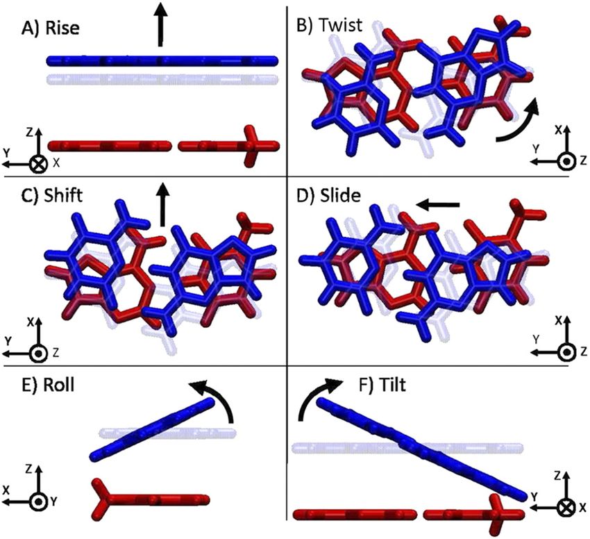
084115-2     Rackers et al.                                                                          J. Chem. Phys. 149, 084115 (2018)

model was the empirical HFD (Hartree-Fock-Dispersion)               dispersion model. We do so first and foremost because it forms
scheme proposed by Scoles and co-workers.21 Another notable         the basis for our damped model, but also because it is instruc-
attempt to describe this phenomenon was undertaken by Tang          tive. One of the defining characteristics of a damped dispersion
and Toennies who introduced a damping function parame-              model, as we shall argue later in the paper, is that it has a
terized to account for the overlap in charge distributions.22       straightforward physical interpretation. Dispersion is correctly
A comprehensive review of dispersion damping functions              said to be a fundamentally non-classical phenomenon, but the
is beyond the scope of this work, but the original Tang             model we use to describe it need not to be so bound. We will
and Toennies report provides a thorough overview of dis-            show that an interpretable model of dispersion can be con-
persion damping functions up to that point. These types of          structed from physical models of atomic polarizability and
formalisms have seen the widest use as dispersion correc-           charge density.
tions to density functional theory (DFT) calculations.23 DFT-
D schemes have used the Tang-Toennies function, as well             A. London dispersion
as various other damping functions proposed by Wu and
Yang,24 Chai and Head-Gordon,25 and Johnson and Becke.26                  For our description of canonical London dispersion
Despite wide use in the DFT community, damped dispersion            energy, we will follow that of Maitland et al.30 The dispersion
functions have been taken up in decidedly fewer molecular           energy between two atoms arises from the interaction between
mechanics models. Notably, the Effective Fragment Poten-            instantaneous dipoles of these atoms. To model this system, we
tial (EFP) model employs a dispersion model that utilizes           consider a simplified one-dimensional Drude oscillator model,
an overlay-based parameter-free modification of the Tang-           as illustrated in Fig. 1.
Toennies damping function.27,28 And recently, Verma et al.                In this representation, each atom is represented by a fixed
proposed using the dispersion part of the DFT-D3 formulation        charge +Q bound by a spring with spring constant, k, and
of Grimme23 as a molecular mechanics model.29 However,              an equal and opposite charge −Q with mass, M. This model
while it has been shown that previous damping functions can         is crude, but it captures the essential elements of the disper-
effectively account for the change in dispersion upon charge        sion interaction. At any point in time, each atom has a dipole
overlap, they do so largely empirically. In the case of the Tang-   moment, µ = Qz (dependent on the atomic polarizability deter-
Toennies damping function, for example, the form is based on        mined by k) and those dipole moments are free to interact with
a Born-Mayer potential described by an empirically fit width        each other.
parameter.                                                                When atom i and atom j are infinitely separated, the
      In this paper, we propose a damped dispersion function        Schrödinger equation for each can be written as
similar in spirit to that of Tang and Toennies but rooted in                         1 ∂ 2 Ψi
                                                                                                              !
                                                                                                2        1 2
a physical model of charge distribution overlap. In previous                                  +     Ei −  kz    Ψi = 0,            (1)
                                                                                     M ∂zi2     ~2       2 i
work, we have shown that a relatively simple model can cap-
ture the physical extent of atomic charge distributions that        where the potential energy term is merely the energy of a sim-
leads to the so-called charge penetration error in electrostatic    ple harmonic oscillator. The same can be written for atom j.
interactions between molecules.11 Here we will show that this       The solutions to this equation can be found trivially, yielding
same model can be used directly and without modification            ground state energies of
to create a dispersion model that is elegantly unified with                            1                     1
the electrostatic model. This unification is possible because                       Ei = ~ω0 and Ej = ~ω0 ,                    (2)
                                                                                       2                    2
both the electrostatic and dispersion terms depend on the den-
                                                                    where the frequency, ω0 , is
sity. The electrostatic term is simply the interaction between                                    r
two static densities, while the dispersion term arises from the                                       k
interaction of densities associated with instantaneous induced                               ω0 =       .                      (3)
                                                                                                     M
dipoles. In this work, we will show that the same rough descrip-    In the complete non-interacting limit, the total energy of the
tion of the density can be used in both cases to great effect.      system is
This will be done in five parts. First, we elucidate the the-                       E(r → ∞) = Ei + Ej = ~ω0 .                 (4)
ory that starts from dipole-dipole interactions and gives rise
to this new damped dispersion function. Second, we describe         This limit in itself is not useful, but if we consider what happens
the methods of the study. Third, we evaluate the performance        when the two atoms get closer, we shall see that it sets a use-
of this function against benchmark Symmetry Adapted Pertur-         ful reference for our potential energy function. If we bring the
bation Theory (SAPT) calculations. Fourth, we will describe         two atoms closer so that they do interact, but not so close that
how the model has been implemented with dispersion particle         their charge distributions overlap, our Schrödinger equation
mesh Ewald (DPME) to boost its efficiency. And finally, we          is no longer trivially separable. The wave equation for two
will discuss the implications of this work and some general
conclusions.

II. THEORY
     To present our new damped dispersion model, we shall
first revisit a simple derivation of the original London                            FIG. 1. Classical model of dispersion.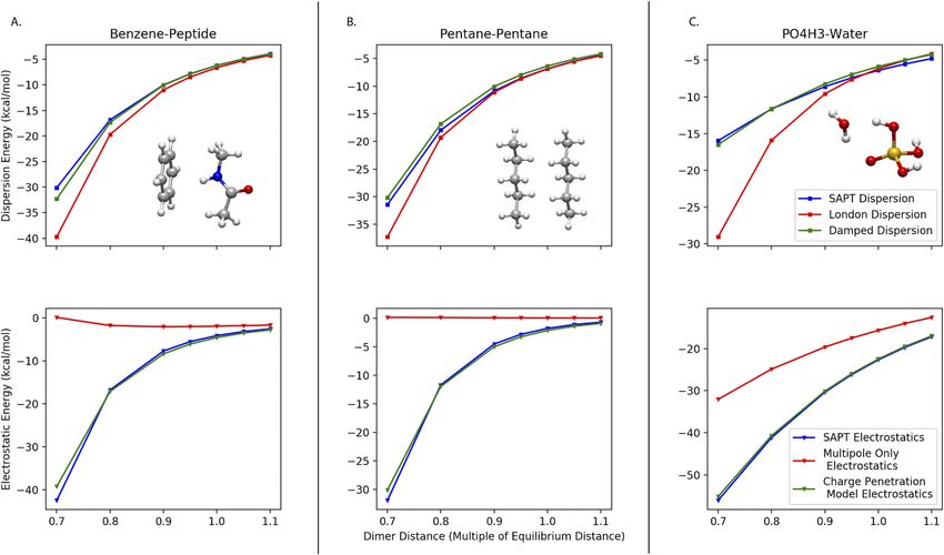
084115-3       Rackers et al.                                                                                   J. Chem. Phys. 149, 084115 (2018)

interacting atoms now includes the electrostatic interaction              One can see that in addition to the simple harmonic oscil-
between the two dipoles and becomes                                       lator terms, a new potential appears in Eq. (5). This is the
                                                                          potential energy at any given instant between the two inter-
1 ∂2 Ψ 1 ∂2 Ψ 2     1 2 1 2
                                               !                          acting instantaneous multipole distributions. For the dipole-
      +      +   E − kzi − kzj − Uelectrostatic Ψ = 0.                    dipole interaction of the simple Drude model of Fig. 1,
M ∂zi2 M ∂zj2 ~2    2     2
                                                                          the form of this potential is easily obtained from simple
                                                                  (5)     electrostatics


                                                                          q q
                                                                            i j      1*                  ~µi · ~rij ~rij · ~µj +
                      Uelectrostatic = Udipole−dipole = ∇∇Uchg−chg = ∇∇            = 3 . ~µi · ~µj − 3                          /.             (6)
                                                                            r       r                              r2
                                                                                       ,                                        -

                                                                                            √
If we plug in the Drude dipoles from Fig. 1, µ = Qz, Eq. (6)                                    1 + x = 1 + 1 2x − 1 8x + · · · ,

                                                                                                                                              (14)
becomes
                                                                        so the total energy becomes
                     1*            (µi r) µj r +     2µi µj                                                Q4 ~ω0
    Udipole−dipole = 3 . µi µj − 3             / = − 3 . (7)                                    E(r) = ~ω0 −        +··· .            (15)
                    r                   r2             r                                                   2r 6 k 2
                       ,                       -
                                                                          The final step is to subtract the energy of infinitely separated
This dipole-dipole energy is the source, as we shall show, of
                                                                          atoms. This gives the dispersion potential energy
the canonical 1/r6 leading term dependence of the dispersion
energy.                                                                                                                     Q4 ~ω0
                                                                                    Udispersion = E(r) − E(∞) = −                    +··· ,   (16)
     Combining Eq. (7) with Eq. (5) yields                                                                                  2k 2 r 6
 1 ∂2 Ψ 1 ∂2 Ψ 2                 1 2 1 2 2µi µj                           where the canonical r6 dependence arises from the first non-
                                                         !
          +          +      E − kzi − kzj −                Ψ = 0.         zero term from the application of the binomial expansion.
 M ∂zi2 M ∂zj2 ~2                2         2        r3
                                                                                It should be noted that while the dipole-dipole interac-
                                                                  (8)     tion is the dominant electrostatic term of Eq. (5), there are
                                                                          terms arising from higher-order multipole interactions as well.
Following the transformation of variables of Maitland, Rigby,
                                                                          The dipole-quadrupole and quadrupole-quadrupole interac-
Smith, and Wakeham, we define
                                                                          tions giving rise to the 1/r8 and 1/r10 potentials are derived
                     zi + zj           zi − zj                            in the Appendix. There are a number of models that use these
               λ1 = √ ,          λ2 = √                   (9)
                         2                 2                              terms, including EFP, SIBFA (Sum of Interactions Between
and rewrite Eq. (8) as                                                    Fragments Ab initio computed), and Misquitta and Stone’s
                                                                          model for small organic molecules.27,31,32 For a perspective
  1 ∂2 Ψ 1 ∂2 Ψ 2
                                       !
                      1        1                                          on the importance of these higher order terms for the case of
        +      +   E − k1 λ i − k2 λ j Ψ = 0, (10)
                            2        2
  M ∂zi2 M ∂zj2 ~2    2        2                                          the neon dimer, the reader is directed to the work of Bytautas
                                                                          and Ruedenberg.33 The latter reference showed that even for
where                                                                     this simple dimer, the 1/r8 and 1/r10 terms are nearly impossible
                       2Q2              2Q2                               to distinguish at reasonable separations. There are odd-power
                 k1 = k +  3
                             , k2 = k − 3 .              (11)
                         r               r                                terms (1/r7 , 1/r9 , etc.) that can be included in the expansion as
Equation (10) is simply a transformed version of the original             well. These arise from the mixing of the even order terms, are
problem of two independent harmonic oscillators. It can be                highly angularly dependent, and spherically average to zero
solved in the same manner giving                                          at long range.34 There has also been recent work on incor-
                                   1                                      porating these terms into dispersion models,35,36 where these
                          E(r) =     ~(ω1 + ω2 ),                (12)     higher-order terms give successively better approximations to
                                   2
                                                                          the exact dispersion energy. As we will show, however, to reach
where                                                                     the stated accuracy goal of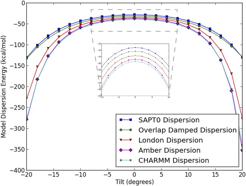
084115-4 Rackers et al. J. Chem. Phys. 149, 084115 (2018)
j
C6i C6 yields the corresponding density,
U dispersion
=− . (17)
r6 qi αi2 ε 0 −α r
This model will be referred to throughout the remainder of ρ(r) = e i . (20)
r
the paper as the London dispersion model. Unfortunately, this
method of approximation starts to break down when the charge These two quantities can be used to approximate the Coulomb
distributions of interacting atoms start to overlap. We will interaction energy between two charge distributions,
handle this situation through the introduction of short-range chg−chg ρi (ri )ρj (rj )
Uelectrostatic = dri drj
damping, but rather than relying on empiricism for the damp- rij
ing function, we look to the underlying electrostatics to provide !
1
a consistent model. = ρi (ri )Vj (rj )dri + ρj (rj )Vi (ri )drj .
2
(21)
B. Short-range electrostatics
Application of the one-center integral method of Coulson39
A long-standing problem in the modeling of electrostatics gives
for molecular mechanics models is the so-called charge pen-
etration error. The error arises when charge distributions of chg−chg qi qj * αj2 αi2
interacting atoms overlap, causing the true electrostatic energy Uelectrostatic = .1 − e−αi r − e−αj r +/.
r αj − αi
2 2 αi − αj
2 2
of the interacting densities to diverge from the point charge or , -
point multipole approximation. We have shown in previously (22)
published studies11,37,38 that a simple hydrogen-like approxi- Equation (22) gives the charge-charge electrostatic energy.
mation of the Coulomb potential does a remarkably good job To get the dipole-dipole energy, recall that the full multipole
at correcting this error. energy of the i-j interaction can be written as
Why is this germane to a study of dispersion? Disper-
sion, as shown above, can be modeled as arising from a
total
Uelectrostatic = U chg−chg + U chg−dipole + U dipole−chg
dipole-dipole interaction. In the context of the multipolar + U dipole−dipole + · · ·
AMOEBA force field, we have shown that the hydrogen-like
= qi Tij qj + qi ∇Tij µj − µi ∇Tij qj
approximation to the Coulomb interaction can be extended
to the interactions between higher-order multipole moments. + µi ∇∇Tij µj + · · · . (23)
In fact, including these corrections for charge-dipole, dipole- For a point-point interaction, T ij is simply 1/r, but for our
dipole, dipole-quadrupole, etc. interactions is essential to the model, direct inspection of Eq. (22) yields
transferability and accuracy of the model.11 Here we show
that the dipole-dipole interaction arising from this earlier 1* αj2 αi2 1 damp
model can be used directly to create a new damped dispersion Tij = .1 − e−αi r − e−αj r +/ = f1 .
r αj − αi
2 2 αi − αj
2 2 r
model. , -
To illustrate where the dipole-dipole damping comes (24)
from, we follow a similar derivation to that of Ref. 11. The We can now apply this new relation for Tij to the definition of
potential due to the electrons for this model is defined as the dipole-dipole energy from Eq. (23),
qi
V (r) = 1 − e−αi r ,
(18) dipole−dipole
Udamp = µi ∇∇Tij µj
r
where r is the distance from the center of the charge distribution ~µi · ~µj
damp damp
3 ~µi · ~rij ~rij · ~µj
and α is a parameter describing the width of the distribution. = f3 − f5 , (25)
r3 r5
Application of Poisson’s equation,
where f 3 and f 5 are the damping terms that come from the
ρ
∇2 V = , (19) derivatives of the f 1 damp term of Eq. (24),
ε0
damp
αj2 αi2
f3 =1− (1 + αi r)e−αi r − 1 + αj r e−αj r ,
αj2 − αi2 αi2 − αj2
(26)
damp
αj2 1
!
αi2
!
1 2 −αj r
f5 =1− 1 + αi r + (αi r) e
2 −αi r
− 1 + αj r + αj r e .
αj2 − αi2 3 αi2 − αj2 3
Now let us compare Eqs. (25) and (6). Clearly the differ- large separations, f 3 and f 5 approach one and we recover
ence between the point dipole-dipole interaction and the new the point interaction. For small density overlaps, f 3 and f 5
model’s dipole-dipole interaction is the damping terms that represent a perturbation that damps the point dipole-dipole
arise from the hydrogen-like model of charge density. For interaction.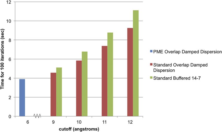
084115-5     Rackers et al.                                                                                             J. Chem. Phys. 149, 084115 (2018)

C. Overlap damped dispersion                                                     remain the same, but instead of inserting the point dipole-
                                                                                 dipole interaction energy into Eq. (5), we now substitute our
     To derive our damped dispersion model, we start from                        damped dipole-dipole interaction from Eq. (25). Following our
the earlier derivation of London dispersion. Equations (1)–(5)                   simple one-dimensional Drude model, we obtain

                                   1 ∂2 Ψ 1 ∂2 Ψ 2
                                                                                                        !
                                                                     1 2 1 2
                                            +          +       E   −   kz −    kz    −  U dipole−dipole Ψ = 0,
                                   M ∂zi2 M ∂zj2 ~2                  2 i 2 j
                                                                                                                                                (27)
                                    dipole−dipole         µi · ~µj
                                                     damp ~            damp
                                                                            3 ~µi · ~rij ~rij · ~µj
                                   Udamp          = f3              − f5                              ,
                                                            r3                         r5
where Udipole-dipole can be simplified to

                                                                         µ  µ
                                                                     damp i j    damp
                                                                                      3(µ i r)   µj r
                                                 Udipole−dipole   = f3      3
                                                                              − f5             5
                                                                                                      .                                             (28)
                                                                          r                  r
Inserting this into the Schrödinger equation yields
                               1 ∂2 Ψ 1 ∂2 Ψ 2                         damp µi µj
                                                                                  !
                                                    1 2 1 2  damp
                                     +      +   E −  kz − kz − 3f  − f              Ψ = 0.                                                          (29)
                               M ∂zi2 M ∂zj2 ~2     2 i 2 j      5     3     r3
This can be solved by the same transformation as the non-damped case discussed earlier where
                                                             2Q2 damp                    2Q2 damp
                                               k1 = k −           f          ,  k2 = k +      f          ,
                                                              r 3 dispersion              r 3 dispersion                                            (30)
                                                 damp             damp      damp
                                               fdispersion   = 3f5     − f3 .
This results in the solution
                                 1
                             E=    ~(ω1 + ω2 ),
                                 2
                                  r          r                                         r             r                                              (31)
                                     k1         2Q2 damp                                   k2                 2Q2 damp
                             ω1 =       = ω0 1 − 3 fdispersion ,                ω2 =          = ω0       1+         f          .
                                     M           r k                                       M                  r 3 k dispersion

Applying the binomial expansion and subtracting the energy                        2. The damping function has a straightforward physical
of infinitely separated atoms yield the damped dispersion                            interpretation: it is the integral of the overlap of between
energy                                                                               charge distributions on interacting atoms.
                                                                                  3. The damping function follows a similar exponential
             damp             Q4 ~ω0  damp  2                                      form as other previously proposed dispersion damping
           Udispersion = −             f          +··· .               (32)
                              2k 2 r 6 dispersion                                    functions.
                                                                                  4. The damping function has no adjustable parameters.
Just as before, for small density overlaps, the leading term                         The parameters are fixed from the electrostatics charge
of Eq. (32) dominates. To convert this into a parameter-                             penetration damping function.
ized molecular mechanics model, we again introduce C 6
                                                                                 As we will show in Sec. IV, this model, in addition to being
parameters, giving our final model energy
                                                                                 theoretically compelling, produces good agreement with dis-
                                        j                                        persion energies from ab initio energy decomposition analysis
                 damp            C6i C6     damp
                                                       2
               Udispersion = −              fdispersion .              (33)      calculations.
                                   r6                   ij

     This model represents an elegant and simple unification of                  III. METHODS
the electrostatics and dispersion models for molecular mechan-
                                                                                       The damped dispersion model we propose requires the
ics force fields. We will refer to this model throughout the
                                                                                 fitting of C 6 parameters. To obtain these parameters, validate
remainder of the paper as the “overlap damped dispersion”
                                                                                 their robustness, and assess the model’s accuracy, we set out
model. It has some important features:
                                                                                 a four-step protocol. First, we assemble a database of repre-
 1. The model retains the canonical 1/r6 asymptotic behavior                     sentative molecular interactions. Second, we perform bench-
    as f tends to unity at large separations.                                    mark ab initio reference calculations on that database. Third,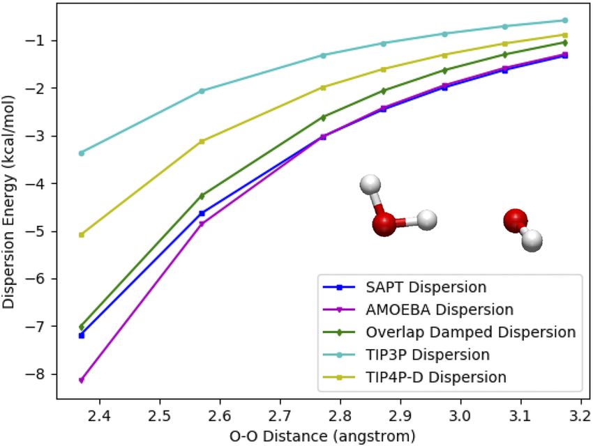
084115-6 Rackers et al. J. Chem. Phys. 149, 084115 (2018)
we fit the parameters of our model to the reference ab initio is a well-established theory with a proliferation of studies ana-
data. Fourth, we assess the robustness of the fit by validation lyzing its accuracy with respect to various orders and basis
of the model on systems outside of the database. sets. We use the SAPT2+ level of theory as defined by Sherrill
For the scope of this study, we intend to parameterize our et al.42 with Dunning correlation consistent basis sets43,44 to
model for the chemical space of biomolecules. To this end, estimate the complete basis set (CBS) limit45 for the SAPT
we use the previously constructed S101x7 database40 for fit- energy components. The SAPT2+ method with large aug-
ting. This database consists of 101 distinct pairs of molecular mented basis sets has been previously shown to give errors rel-
dimers. For each of these dimers, seven points along the dis- ative to coupled-cluster single, double and perturbative triple
sociation curve are established at 0.7, 0.8, 0.9, 0.95, 1.0, 1.05, excitations [CCSD(T)]/CBS of about 0.3 kcal/mol. This was
and 1.1 times the equilibrium intermolecular distance. Details chosen over the cheaper to compute SAPT0 method, which
on how the structures were generated are available in Ref. 37. gives errors of around 0.5 kcal/mol. In order to minimize the
The dimers in this set represent a cross section of typical inter- difference between our SAPT calculations and gold-standard
actions found in protein and nucleic acid systems. We note CCSD(T), we evaluated the residual
that the points in the dataset at 0.7x the equilibrium distance CCSD(T )/CBS
SAPT 2+/CBS SAPT 2+/CBS
are important despite the fact that they are rarely sampled in R = Etotal − Enon−dispersion + cEdispersion , (34)
condensed phase simulations for most systems. These points
are included to ensure that the shape of the potential at the where (Enon-dispersion + Edispersion ) represents the total SAPT2+
closest sampled points (often 0.8x the equilibrium distance) is energy, with a scale factor, c, introduced as a parameter. Min-
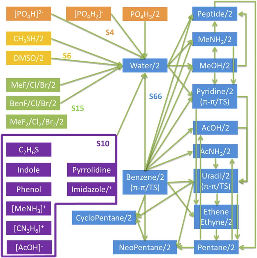
accurately captured. A summary of all the pair interactions is imizing this residual with respect to c yielded a scale factor of
presented in Fig. 2. c = 0.89 that is used to scale all dispersion energies. For further
In order to parameterize our model, a set of dispersion ref- details on the construction of the reference data for S101x7,
erence data is required. Because dispersion is not a physical please see Ref. 37. The Psi4 program was used to perform all
observable, we must rely on an ab initio energy decomposition SAPT calculations.46–48 All structures and reference data are
analysis (EDA) to generate our reference data. We have cho- available at the S101x7 online repository.40
sen Symmetry Adapted Perturbation Theory (SAPT)41 for this To obtain C 6 parameters, we performed a nonlinear least
purpose. SAPT has a number of features that makes it a rea- square fit of the SAPT dispersion reference data using a
sonable choice. First, SAPT is a perturbation theory approach Levenberg-Marquardt algorithm implemented in the Tinker
that takes the electron density of monomers as its unperturbed molecular mechanics software package. To test the robust-
state. This is an exact analogy to molecular mechanics mod- ness of this parameterization, we leave out some of the
els where distributed multipoles are calculated from monomer data points and repeat the fit. The model with the new
densities. Second, because of this correspondence, SAPT is the parameters is then evaluated on the excluded points. As a
theory that was used to generate the parameterization of the validation test case, we also evaluate the performance of
electrostatic model referenced in Sec. II. Using SAPT here as the model on previously published nucleic acid interaction
well ensures a straightforwardly unified model. Finally, SAPT data.49
The last part of the study is the evaluation of the disper-
sion particle mesh Ewald (DPME) method. DPME has been
implemented in a locally modified version of Tinker and is
available through the Tinker GitHub site.50 To evaluate the
efficiency of this implementation, the DPME method is tested
on a 36 Å periodic cube containing 1600 water molecules. The
PME summation was performed with a ∼1 Å grid, 5th order
B-splines, and an Ewald coefficient of 0.4. Timings are com-
puted on a 6-core, 2.66 GHz Intel Xeon processor for 100
energy evaluations using standard (non-Ewald) and DPME
overlap damped dispersion.
IV. RESULTS
A. Model accuracy
The question that we are attempting to answer in this study
is whether or not a damped dispersion model that is consis-
tent with an underlying electrostatic model is demonstrably
more accurate relative to ab initio data than simpler counter-
parts. To test this question, we employed a two-step approach.
First, we compared the pure London dispersion model with
our new overlap damped dispersion model on the S101x7
FIG. 2. Dimer pairs in the S101 database. Arrows indicate heterodimers,
database. Then we compared these models to recently pub-
while “/2” indicates a homodimer. Reprinted with permission from Wang et al.,
J. Chem. Theory Comput. 11, 2609–2618 (2015). Copyright 2015 American lished work fitting the S101x7 database with a buffered 14-7
Chemical Society. potential function.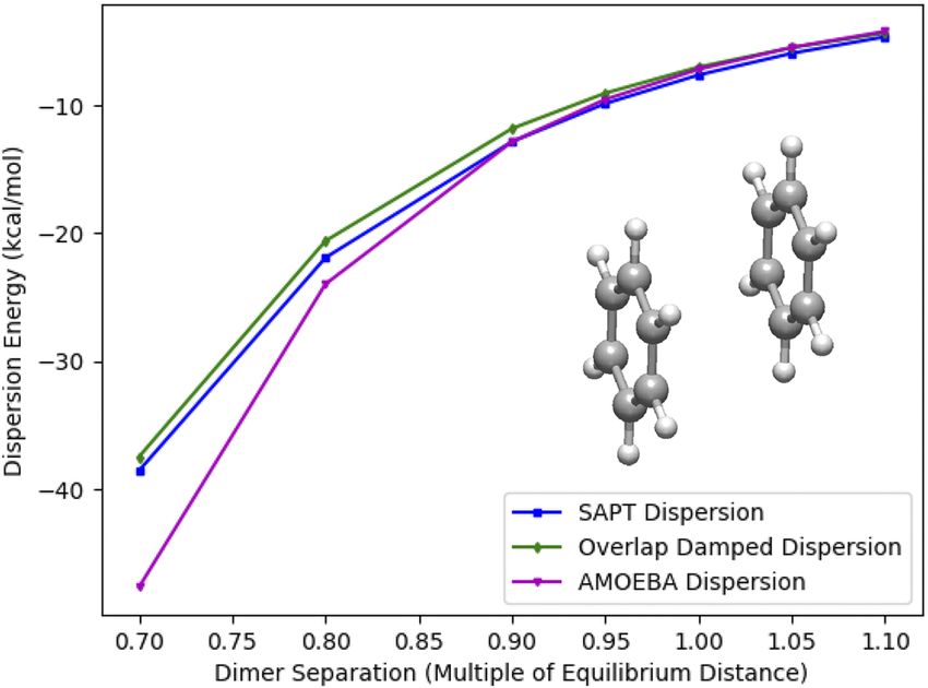
084115-7        Rackers et al.                                                                                       J. Chem. Phys. 149, 084115 (2018)

TABLE I. Goodness of the fit on the S101x7 database (kcal/mol).                  TABLE II. Fixed electrostatic damping parameters.

                                              London         Overlap damped      Element                             Atom class                    α (Å 1 )
                                             dispersion        dispersion
                                                                                                                Non-polar                           3.2484
Total root mean square error (RMSE)             1.19               0.52          Hydrogen (H)                   Aromatic                            3.4437
Short-range RMSE (0.7–0.8× equil dist)          1.52               0.65                                         Polar, water                        3.2632
Long-range RMSE (0.9–1.1× equil dist)           1.04               0.46
                                                                                                                sp3                                 3.5898
                                                                                 Carbon (C)                     Aromatic                            3.2057
                                                                                                                sp2                                 3.1286
      To compare the damped and non-damped 1/r6 dispersion
potentials, we fit both to the SAPT2+ dispersion values from                                                    sp3                                 4.0135
the S101x7 database. The results of these fits are presented in                  Nitrogen (N)                   Aromatic                            3.6358
                                                                                                                sp2                                 3.7071
Table I and Fig. 3.
      Clearly the overlap damped dispersion potential performs                                                  sp3 , hydroxyl, water               4.1615
better on this set of data, displaying a total root mean square                  Oxygen (O)                     Aromatic                            4.3778
error of 0.52 kcal/mol, as opposed to 1.2 kcal/mol for the                                                      sp2 , carbonyl                      3.7321
pure London dispersion function. Figure 3 illustrates how the
                                                                                 Phosphorous (P)                Phosphate                           2.7476
overlap damped dispersion model consistently fits the SAPT
dispersion data better than the non-damped model over a range                    Sulfur (S)
                                                                                                                Sulfide                             3.3112
of interactions energies.                                                                                       Sulfur IV                           2.6247
      Moreover, the difference in fit quality between the short-                 Fluorine (F)                   Organofluoride                      4.4675
range and long-range points shown in Table I is much smaller
for the overlap damped dispersion model. This seems to indi-                     Chlorine (Cl)                  Organochloride                      3.4749
cate that the damping is having the short-range effect we hoped                  Bromine (Br)                   Organobromide                       3.6696
it might. This issue will be examined further in the robustness
tests.
      It is instructive to note exactly what is and is not being
                                                                                 damped dispersion model exhibits a smoother variation within
fit in these two models. For both models, the only parame-
                                                                                 classes.
ters being fit are one C 6 coefficient per atom class. (Atom
                                                                                      The fact that a similar set of parameters produces a
class definitions can be found in Table II. They are identi-
                                                                                 damped dispersion model that yields a fit that is 0.5 kcal/mol
cal to those defined in Ref. 11.) It bears emphasizing that for
the overlap damped dispersion model, the damping parame-
ters [α i in Eq. (26)] are not allowed to vary; they are fixed                   TABLE III. Model C6 parameters.
at the values determined in Ref. 11. These values, recapit-
ulated here in Table II, describe the physical extent of an                                                                       London          Damped
                                                                                                           Atom                dispersion C6   dispersion C6
atom’s electron distribution. They were fit to the SAPT elec-
                                                                                 Element                   class               (Å6 kcal/mol)   (Å6 kcal/mol)
trostatic energies of the same S101x7 database in the previ-
ous study. A comparison of the C 6 parameters between the                                           Non-polar                      3.4118         6.3960
damped and non-damped models in Table III shows that the                         Hydrogen (H)       Aromatic                       4.7993         5.7678
                                                                                                    Polar, water                   0.9114         5.1133

                                                                                                    sp3                           28.5333        18.1732
                                                                                 Carbon (C)         Aromatic                      23.2125        23.3605
                                                                                                    sp2                           26.1301        23.0103

                                                                                                    sp3                           33.6562        21.4927
                                                                                 Nitrogen (N)       Aromatic                      18.2114        19.7421
                                                                                                    sp2                           30.6586        19.4543

                                                                                                    sp3 , hydroxyl, water         25.5861        15.1656
                                                                                 Oxygen (O)         Aromatic                      25.2794        14.8569
                                                                                                    sp2 , carbonyl                23.1181        18.4344

                                                                                 Phosphorous (P)    Phosphate                     46.4113        44.8658

                                                                                                    Sulfide                       62.1844        52.8970
                                                                                 Sulfur (S)
                                                                                                    Sulfur IV                     39.0781        59.2558

                                                                                 Fluorine (F)       Organofluoride                15.0568        13.6549

                                                                                 Chlorine (Cl)      Organochloride                44.4420        45.7799
FIG. 3. Damped and undamped dispersion models against SAPT2+ disper-
sion energies. The diagonal y = x dashed line indicates perfect agreement. The   Bromine (Br)       Organobromide                 59.9587        62.0655
overlap damped dispersion model produces a significantly improved fit.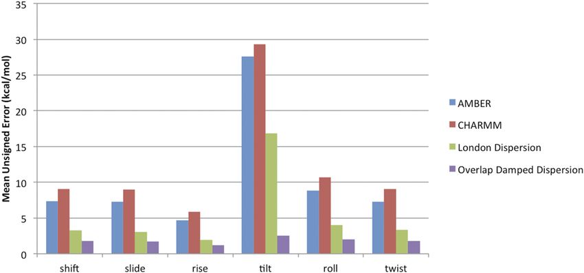
084115-8     Rackers et al.                                                                              J. Chem. Phys. 149, 084115 (2018)

better than the non-damped model, despite having the exact
same number of fitting parameters, is instructive. It shows
us that the quality is not due to any extra flexibility in the
fitting procedure. This hints that our model may be seizing
some of the same physical reality captured in the electrostatics
model.
      The London dispersion model is widely used, but it is cer-
tainly not the only simple dispersion model used in molecular
mechanics force fields. One alternative is Halgren’s buffered
14-7 potential.18 As discussed in Sec. II, the 1/r6 term is only
the first term in the expansion of the dispersion energy. The
buffered 14-7 potential,
                                 !7
                         1+δ         1+γ
                                                !
            XX                                            rij
   UvdW =           ε ij                    − 2   , ρij =     ,
            vdw i,j
                         ρij + δ    ρij + γ
                                       7                  σij
                                                              (35)    FIG. 4. vdw2016 against SAPT2+ dispersion. The diagonal y = x dashed
                                                                      line indicates perfect agreement. The vdw2016 model systematically under-
attempts to accommodate higher order terms by means of                estimates the magnitude of the dispersion energy.
the buffered 1/r7 attractive term to describe dispersion. The
buffered 14-7 van der Waals potential has been used in a num-
ber of force fields, including AMOEBA, for which a large              14-7 van der Waals form to the S101x7 dataset, vdw2017,
amount of analysis involving the S101x7 database has already          where the exchange-repulsion and dispersion components
been done.                                                            were fit independently. The results of this fit are shown in
      In a recent study, Qi, Wang, and Ren fit the buffered 14-7      Fig. 5.
van der Waals potential to the sum of the exchange-repulsion               One can see that the systematic deviation in dispersion
and dispersion data from the S101x7 database yielding a               that plagues the vdw2016 model is largely alleviated in the
model they call “vdw2016.”51 Given the quality of the total           new fit. However, the root mean square error for vdw2107 dis-
van der Waals energy reported, we set out to see how the              persion remains at 1.6 kcal/mol. This occurs despite preserving
corresponding dispersion energies compared to 1/r6 derived            the extra flexibility of having 28 atom classes. This seems to
functions.                                                            show that while the buffered 14-7 may have a fortunate can-
      To assess the performance of the dispersion part of the         cellation of errors for the total van der Waals energy, a 1/r6
vdw2016 model, we performed calculations using only the               asymptotic function is a more natural fit to the pure dispersion
attractive part of the buffered 14-7 potential defined in Eq. (35).   interaction.
The vdw2016 model differs slightly from the damped and non-                Comparing the overall fits of the Halgren dispersion
damped 1/r6 dispersion models in its number of atom classes.          potentials to the (damped or non-damped) London disper-
Where we define just 18 atom classes for the molecules in             sion potentials, it is clear that the latter produce a better fit to
S101, Qi, Wang, and Ren found that they need 28 to accu-              the S101x7 dataset. Since the empirical buffered 14-7 poten-
rately model the van der Waals energy. For each class, they           tial seems to offer no advantage in accuracy for dispersion,
allowed two parameters to vary: the well depth, ε, and radius,        there is no reason to further pursue it as a viable interpretable
σ. Despite this greater flexibility in parameters, the vdw2016
model performs very poorly on predicting the dispersion part
of the van der Waals energy. As is clearly seen in Fig. 4, it is
not nearly attractive enough.
      This is unsurprising given the nature of the fit that was
performed. Since the target data were the sum of the exchange-
repulsion and dispersion energies, the fit is highly skewed by
the exchange-repulsion energy. The exchange-repulsion can
often be an order of magnitude large than dispersion, espe-
cially at short-range, and thus drives values obtained for the
fit. This does not mean that vdw2016 does not make an ade-
quate empirical total van der Waals model (indeed buffered
14-7 has almost always been used in its totality), but it does
mean that this parameterization will not work as a stand-alone
dispersion model if the goal is to reduce the cancellation of
errors.
      While the vdw2016 model has been shown to yield good
van der Waals energies, it does so to the detriment of hav-           FIG. 5. vdw2017 dispersion against SAPT 2+ dispersion energies. The diag-
ing a separate and interpretable dispersion model. To attempt         onal y = x dashed line indicates perfect agreement. The vdw2017 model RMS
to remedy this, we performed a second fit of the buffered             error is 1.6 kcal/mol.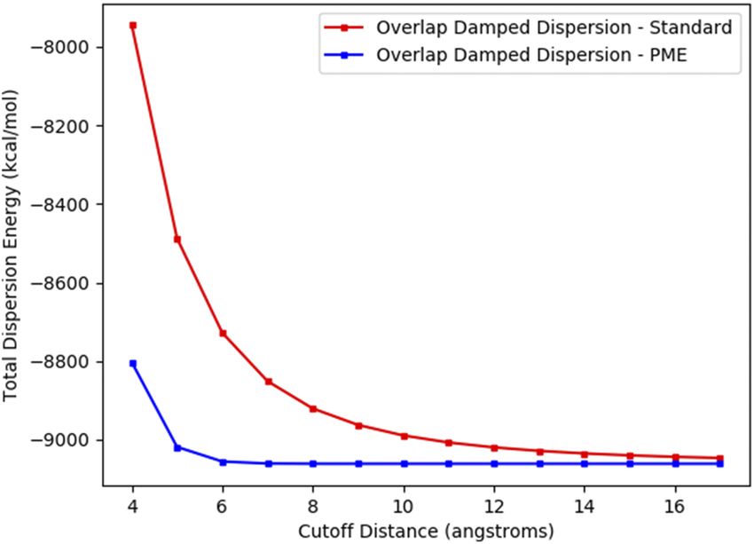
084115-9      Rackers et al.                                                                              J. Chem. Phys. 149, 084115 (2018)

dispersion model for the purposes of this study. The next                 of the London dispersion model is over 5 kcal/mol. These
step is to assess whether the advantage in the accuracy of the            errors are clearly caused by the inability of a simple 1/r6 func-
damped dispersion model is worth the extra complexity and                 tion to adequately describe both the asymptotic and overlap
computational effort.                                                     regimes. Moreover, it is clear from Table IV that the overlap
                                                                          damped dispersion model is not sacrificing accuracy in the
                                                                          asymptotic regime, where it is actually slightly better than the
B. Model robustness
                                                                          London dispersion model. A handful of illustrative examples
      Although the overlap damped dispersion model shows a                show how the London dispersion model fit to near-equilibrium
better fit to the S101x7 dispersion dataset, we would like to be          points systematically predicts the dispersion energy to be too
sure that this advantage over the simpler London dispersion               attractive. Figure 6 shows three examples where this effect is
model is robust. To test this point, we employed two separate             pronounced.
validation assessments. First, we interrogated the quality of the              The pentane-pentane, benzene-peptide, and water-PO4 H3
fit with regard to intermolecular distance. Here our aim was              interactions are all examples of important component interac-
to ascertain which of the two functions is a more natural fit to          tions in biology. They also exhibit the importance of damping
the data. Second, we applied both models to cases outside of              the dispersion energy at short range for an ab inito-based force
the S101 suite of dimers.                                                 field. Clearly, including the damping function from the elec-
      The S101x7 dataset contains sets of dimers arranged at              trostatic model improves the agreement with SAPT dispersion
seven different intermolecular distances (0.7, 0.8, 0.9, 0.95,            data at the closest points.
1.0, 1.05, and 1.1 times the equilibrium distance). Because                    We suggest that the effectiveness of this damping is fun-
this data set includes a good amount of information about close           damentally tied to the overlap in charge distributions. If we
contact points, we want to be sure that our models fit the short-         compare the non-damped London dispersion curves with their
range points well without sacrificing asymptotic behavior. To             corresponding non-damped electrostatic curves (no charge
judge the long-range fit, we excluded all of the 0.7 and 0.8 times        penetration correction) in Fig. 6, we see that the divergence
equilibrium data points and then reoptimized the parameters.              of non-damped energies from their SAPT counterparts occurs
The results, presented in the “long-range” entries of Table IV,           at roughly the same separation. This suggests that deviation
show that for this near-equilibrium regime, the London disper-            from the 1/r6 asymptotic behavior in the dispersion energy at
sion and overlap damped dispersion models give comparable                 short-range is also attributable to the overlap in charge dis-
fits.                                                                     tributions. We know that the point multipole expansion model
      The test of robustness is to then use the parameters                for electrostatic interactions is rigorously accurate until charge
that come out of the near-equilibrium fits and evaluate each              distributions begin to overlap. The fact the divergence in the
model on the close-contact points that were left out of the               point dipole derived dispersion energy occurs at a similar
fit. This shows how well the shape of the function matches                distance suggests that the same effect is driving this phe-
the intrinsic shape of the dispersion dissociation curve at               nomenon. Moreover, the fact that the exact same parameters
short range. As can be seen in Table IV, there is a difference            can be used to accommodate the change from the asymp-
between the London dispersion and overlap damped dispersion               totic behavior for both electrostatics and dispersion indicates
models.                                                                   that these are separate manifestations of the same physical
      The total RMS error of the overlap damped dispersion                reality.
model increases modestly when the close-contact points are                     Although the London dispersion model may be simpler
included, as should be expected since these points were not               and computationally less expensive than the overlap damped
included in the fit. The total RMS error of the non-damped                dispersion model, it is clear from this robustness test that the
London dispersion model, however, rises dramatically. While               latter provides a much better description of the dispersion
the long-range quality of the fit (those points that were included        interaction that spans both the close contact and asymptotic
in the fit) is good for both models, the short-range quality              regimes. For the S101x7 dataset, generally, the 0.8x points
(those points not included in the fit but included in the robust-         represent the closest intermolecular distance for liquids under
ness test) is very different between the two models. The RMS              ambient conditions. The robustness test shows that a force
error on the short-range test points with the overlap damped              field using the overlap damped dispersion model will rely less
dispersion model is less than 1 kcal/mol, but the RMS error               on the cancellation of errors in this area than an undamped
                                                                          model. Importantly, we note that the overlap damped disper-
                                                                          sion model retains the 1/r6 dependence at long range as the
TABLE IV. Dispersion model robustness test (kcal/mol).
                                                                          damping factor quickly approaches unity when charge distri-
                                           London        Overlap damped   butions no longer overlap. This gives us confidence that the
                                          dispersion       dispersion     shape of the function is well suited to the intrinsic shape of the
                                                                          dispersion dissociation curve.
Total root mean square error (RMSE)         3.12              0.67
Total mean signed error (MSE)               0.91              0.31
Short-range RMSE (0.7–0.8× equil dist)      5.55              0.84        C. Model analysis and validation
Long-range RMSE (0.9–1.1× equil dist)       1.15              0.59
Short-range MSE (0.7–0.8× equil dist)       2.71              0.12            Having established the capability of the overlap damped
Long-range MSE (0.9–1.1× equil dist)        0.20              0.38        dispersion model for short-range interactions, we can ask
                                                                          how well this model performs on specific important systems.
084115-10 Rackers et al. J. Chem. Phys. 149, 084115 (2018)
FIG. 6. Examples of dispersion (top row) and electrostatic (bottom row) corrections for charge density overlap in (a) benzene-peptide, (b) pentane-pentane, and
(c) water-PO4 H3 interactions. The x-axis indicates dimer intermolecular distance as a fraction of each dimer’s equilibrium separation. In all three examples, the
undamped “classical” model diverges from the ab initio result at short range, while the damped model follows the ab initio curve closely.
Dispersion plays an important role in a range of biomolec- near equilibrium, this model produces excellent agreement,
ular interactions, and one should hope a good model would but at short range, the dispersion energy becomes too negative.
describe such interactions accurately. Two instructive exam- While the absolute energy error may not be large for these close
ples are water-water interactions and benzene stacking inter- points, one can see that the error in the slope is much greater.
actions. Both also happen to be instances where charge density At an O–O distance of ∼2.6 Å, for example—well sampled
overlap plays a role in their short-range interactions.
The balance between water-water and water-biomolecule
interactions is known to be important to accurate simulations
of biomolecules. Recently, a study by Piana and co-workers
demonstrated that simulations with a few commonly used
water models overpredict the compactness of disordered and
partially disordered proteins.52 They suggest that this occurs
because these typical water models underestimate water-water
and water-protein dispersion interactions relative to ab initio
dimer calculations. This conclusion may be overstated since
for the TIP3P and SPCE models discussed, this underesti-
mation is largely handled through the cancellation of errors
within the rest of the force field. A goal of our work, however,
is to reduce this reliance on such cancellation. The over-
lap damped dispersion model directly addresses this problem
through an accurate prediction of the water dimer dispersion
energy curve. As shown in Fig. 7, the damped model gives
good overall agreement with the shape of the SAPT dispersion
data. FIG. 7. Performance of various water dispersion models against SAPT2+
Also shown in Fig. 7 is the quality of the fit of the dispersion. Model dispersion energies are compared to SAPT2+ dispersion
AMOEBA water0319 model. Since this AMOEBA model is energies for a range of intermolecular distances of the water dimer. TIP3P53
and TIP4P-D52 are undamped ∼1/r6 models, AMOEBA is the attractive,
polarizable, one would expect the dispersion part of its van
∼1/r7 , component of the buffered 14-7 potential with parameters from the
der Waals function should be close to the ab initio dispersion water03 force field,19 and the overlap damped dispersion model is from this
energy due to less reliance on the cancellation of errors. Indeed, work.084115-11 Rackers et al. J. Chem. Phys. 149, 084115 (2018)
in ambient water 54 —one can see that the water03 dispersion Finally, to check that the success at accurately fitting, the
force is slightly too attractive. Recent work has suggested that S101x7 dataset is not the result of overfitting, we employ a
the cancellation of errors is responsible for the condensed validation test on a system outside of the training set. For this
phase behavior of AMOEBA water,55,56 but as these compen- purpose, we chose to test the dispersion component of nucleic
satory components are removed for the next generation of the acid base stacking interactions. In previously published work,
model, the error in the dispersion becomes more important to Parker and Sherrill performed SAPT energy decomposition
address directly. It is not novel to suggest that modeling the analysis calculations on a set of nucleic acid structures to eval-
short and long-range dispersion interactions simultaneously uate the performance of current force fields. In order to assess
requires a damping function. What is shown here, however, how well a given model reproduces the energy components
is that a simple, rationally constructed, and minimally param- of base stacking interactions, Parker and Sherrill performed
eterized model yields excellent agreement for this important SAPT calculations at equilibrium and near equilibrium geome-
interaction. tries of all ten possible two base-pair steps of DNA: AATT,
Another example interaction of importance in biomolec- ACGT, AGCT, ATAT, CATG, CGCG, GATG, GCGC, GGCC,
ular modeling is the benzene “pi-stacking” interaction. In and TATA. To generate trial geometries, Parker and Sherrill
addition to being an important exemplar for the nucleic acid systematically varied the six geometrical degrees of freedom
structure and drug binding, this interaction falls into the quali- illustrated in Fig. 9 (shift, slide, rise, tilt, roll, and twist) for each
tative “dispersion-bound” category,57 so accurately modeling base-pair step. See Ref. 49 for structure generation specifics
it is imperative for a dispersion model. Figure 8 shows the and calculation details.
performance of the overlap damped dispersion model against To see how our model measures up, we compare the
SAPT. published nucleic acid SAPT dispersion energies with the dis-
One can see that the agreement of the overlap damped persion energies predicted by our overlap damped dispersion
dispersion model with the SAPT data is excellent across all model using atom types, as defined in Table III. The results for
benzene dimer separations. As was observed for the water this test set are shown in Fig. 10.
dimer, the AMOEBA model produces good agreement near There are two important features to point out in the figure.
equilibrium, but characteristically deteriorates at short range. First, one will notice that the London dispersion model per-
In particular, the divergence begins at ∼0.85 of the equilib- forms better than either the Amber or CHARMM nucleic acid
rium separation or a ∼3.2 Å C–C distance. This distance is dispersion models despite having an identical functional form.
a close contact for liquid benzene at room temperature and This, as noted by Parker and Sherrill, is primarily due to the
1 atm—it falls near the start of the radial distribution func- cancellation of errors in the partial charge models. These mod-
tion.58 As a model system, it is also close to the stacking els do not explicitly include the effects of charge penetration,
distance between bases in B-DNA, ∼3.3 Å. Figure 8 shows that so the dispersion function is called upon to absorb some of the
for small but relevant distances like this, the shape of SAPT errors in the electrostatics. What Parker and Sherrill find, how-
dispersion is more closely matched by the overlap damped ever, is that while this cancellation of errors strategy produces
dispersion Model. Although less dramatic than with electro- total energies within 1 kcal/mol relative to dispersion-weighted
statics, the deviation at a short range of the London dispersion CCSD(T∗∗ ) for structures near B-form DNA, the error in the
model is due to the same phenomenon that drives the diver- total energy across the range of potential energy surface scans
gence in the electrostatics of the benzene dimer. Figure 8 shows is closer to 2 kcal/mol with some errors over 10 kcal/mol
us that the same treatment can be applied to fix the errors in even for attractive points on the surface. One can see from
both classical models.
FIG. 8. Benzene dimer dispersion. Model dispersion energies are compared FIG. 9. Illustration of the six degrees of freedom explored for nucleic acid
to SAPT2+ dispersion energies for a range of intermolecular distance of the structures. The example shown is for the AC:GT base step. Reprinted with
benzene dimer. The AMOEBA model functional form is the same as in Fig. 7, permission from Parker and Sherrill, J. Chem. Theory Comput. 11, 4197–4204
with parameters taken from the AMOEBA09 force field. (2015). Copyright 2015 American Chemical Society.084115-12 Rackers et al. J. Chem. Phys. 149, 084115 (2018)
FIG. 10. Mean unsigned error in dispersion energy for nucleic acid structures. Model error is relative to SAPT for each of the six structural parameters. The
overlap damped dispersion model reduces the error in the dispersion across all six degrees of freedom. Amber and CHARMM results from Ref. 49.
Fig. 10 that parameterizing a 1/r6 (London dispersion) model energy with good precision. However, as one changes the
directly to SAPT reduces some of the need for the cancel- tilt angle in either direction, the dispersion energy of the
lation of error, but not all. The second and more important undamped model diverges quickly from the SAPT while the
feature one observes is the agreement throughout the poten- overlap damped dispersion model follows the shape of the
tial energy surface of the overlap damped dispersion model. SAPT curve with fidelity. This trend holds across all six
In addition to relieving itself of the cancellation of errors bur- degrees of freedom and all ten base pair steps. Plots like Fig. 11
den, one can see that the damped model provides a minimum for each combination are available in the supplementary mate-
factor of two improvements in the mean unsigned error over rial. The divergence observed for non-damped models matters
the undamped London dispersion model for every degree of because it is not simply confined to high total energy areas of
freedom. This has little to do with the behavior of the disper- the DNA potential energy surface. In fact, Parker and Sher-
sion energy at equilibrium; the divergence occurs primarily for rill showed that for the stacked A-C pair (one half of the
structures where the electron densities of the two base-pairs CATG base step) at a tilt angle of −15◦ , the total energy is
start to overlap. −5 kcal/mol. This is only 0.5 kcal/mol above the minimum
As an instructive example, take the change in dispersion total energy of −5.5 kcal/mol. Figure 11 suggests that in order
energy with respect to the tilt angle for the CATG base step to accurately model this region of the potential energy sur-
shown in Fig. 11. face without large cancellation of errors, a damped dispersion
One can see that at equilibrium, both the London and over- model is necessary.
lap damped dispersion models predict the SAPT dispersion
V. DISPERSION PARTICLE MESH EWALD
SUMMATION
Accuracy and efficiency are both important features of a
molecular mechanics model. A good dispersion model must
not only be accurate, but also fast to compute. While the accu-
racy of the overlap damped dispersion model has been solidly
established in this paper, the exponentials required for its eval-
uation have the potential to slow potential energy calculations.
To make the overlap damped dispersion model computation-
ally efficient and tractable for use in biomolecular simulations,
we have implemented the model with particle mesh Ewald
(PME) summation in the Tinker molecular mechanics soft-
ware package. In this section, we present a brief overview of
the damped dispersion PME implementation and show how
this implementation provides a substantial speed and accuracy
improvement over the standard cutoff-based van der Waals
FIG. 11. Dispersion energy of CATG interaction vs. tilt. The non-damped dis- implementation.
persion models uniformly overestimate the magnitude of the dispersion energy
as the angle varies from equilibrium in either direction. The overlap damped Ewald summation is classically considered to be pri-
dispersion model predicts the shape of the SAPT curve at both equilibrium marily a solution to the pairwise long-range electrostatics
and near-equilibrium geometries. problem. The Σ1/r electrostatic potential is conditionally084115-13 Rackers et al. J. Chem. Phys. 149, 084115 (2018)
convergent which makes direct computation of the electro- brief summary simply to show that the inclusion of a damp-
static energy of a periodic system difficult. To circumvent ing term in this case does not change the ability to use the
this problem, Ewald methods split the sum into short-range method.
and long-range parts, with short-range part being computed The total dispersion energy, as given by Eq. (33) is
directly and the long-range via Fourier transformation. This
separation not only makes periodic calculations possible, but X Ci Cj 2
damp 6 6 damp
also increases the speed with which the energy and gradient Udispersion = − fdispersion . (36)
i,j rij6 ij
can be evaluated.
The same method can be applied to the dispersion energy This can be split into a short-range part, a long-range part, and
calculation. Here we note that the following derivation is a “self” term,
by no means original. In fact, Essman and co-workers pro-
dispersion dispersion dispersion dispersion
posed the possibility of using particle mesh Ewald summation Utotal = Ushort−range + Ulong−range + Uself , (37)
for dispersion in their 1995 paper describing the method of
smooth particle mesh Ewald summation.59 We present here a with
X Ci Cj 2 !
1 4 4 −β2 rij2
dispersion 6 6 damp
Ushort−range = fdispersion 1 + β 2 rij2 + β rij e , (38a)
i,j rij6 ij 2
2π 9/2 X
" √
#
dispersion 1
2 (−(π |m |/β)2 + πerfc(π |m |/β))
Ulong−range = |m| 3 1 − 2(π|m|/ β) e Ŝ(m)Ŝ(−m), (38b)
3V m,0 2(π|m|/ β)3
2
dispersion β 6 X 2 β 3 π 3/2 *X +
Uself =− Ci + Ci . (38c)
12 i 6V , i -
Equations (38a) and (38b) are commonly known as the direct One can see that for cutoffs longer than 6 Å, the energy of
space sum and reciprocal space sum, respectively. The vari- the PME implementation is constant due to the fact that f damp
able, β, is the parameter determining the Gaussian width, m is effectively unity for all atom pairs outside of this radius. For
is defined by the reciprocal lattice vectors, a, as m = m1 a1 ∗ our model, we chose this cutoff of 6 Å to balance the direct and
+ m2 a2 ∗ + m3 a3 ∗ , and V is the volume of the unit cell. The reciprocal space computational effort. Comparing the PME
structure factor, S, is defined for dispersion as and non-PME curves in Fig. 12 illustrates an obvious advan-
X tage of using Ewald summation for dispersion interactions.
Ŝ = Cj ei2π (m·rj ) . (39) While the non-PME curve converges to the asymptotic total
j
The summation in Eq. (38b) is handled in the same manner
as the reciprocal space sum for electrostatics. Tinker uses the
FFTW (Fastest Fourier Transform in the West) package to per-
form the needed Fourier transforms.60 To speed the calculation
and because the dispersion energy decreases quickly with dis-
tance, Eq. (38a), the direct space sum, is truncated at a fixed
distance.
For simple dispersion PME, the choice of direct space
cutoff matters very little; one simply chooses a cutoff that bal-
ances computational effort between direct space and reciprocal
space. For overlap damped dispersion PME, however, some
care must be taken with the choice. This is because Eqs. (38a)–
(38c) as written do not strictly sum to Eq. (36). This imbalance
is caused by the presence of the damping function in the direct
space sum, without an equivalent component in the recipro-
cal space. In practice, however, this is easily overcome with a
rational choice of cutoff distance. The function f damp goes to FIG. 12. Cutoff distance convergence of the overlap damped dispersion
unity very quickly with distance (much faster than 1/r6 goes model. The total dispersion energy of a 36 Å water box is shown for the stan-
dard and particle mesh Ewald (PME) implementations of the overlap damped
to zero), so reasonable cutoff distances are easy to obtain. dispersion model. The cutoff of the PME implementation refers to the cut-
Figure 12 shows dispersion energy as a function of cutoff off of the real space summation. Computational details are enumerated in
distance. Sec. III.You can also read