Simulations of anthropogenic bromoform indicate high emissions at the coast of East Asia
←
→
Page content transcription
If your browser does not render page correctly, please read the page content below
Atmos. Chem. Phys., 21, 4103–4121, 2021
https://doi.org/10.5194/acp-21-4103-2021
© Author(s) 2021. This work is distributed under
the Creative Commons Attribution 4.0 License.

Simulations of anthropogenic bromoform indicate
high emissions at the coast of East Asia
Josefine Maas1,a , Susann Tegtmeier1,2 , Yue Jia1,2 , Birgit Quack1 , Jonathan V. Durgadoo1,3 , and Arne Biastoch1,3
1 GEOMAR      Helmholtz Centre for Ocean Research Kiel, Kiel, Germany
2 Instituteof Space and Atmospheric Studies, University of Saskatchewan, Saskatoon, Canada
3 Faculty of Mathematics and Natural Sciences, Kiel University, Kiel, Germany
a now at: Helmholtz-Zentrum Geesthacht, Institute of Coastal Research, Geesthacht, Germany

Correspondence: Susann Tegtmeier (susann.tegtmeier@usask.ca)

Received: 30 October 2019 – Discussion started: 27 January 2020
Revised: 23 January 2021 – Accepted: 25 January 2021 – Published: 18 March 2021

Abstract. Bromoform is the major by-product from chlori-          FLEXPART simulations show mean anthropogenic bromo-
nation of cooling water in coastal power plants. The number       form mixing ratios of 0.4–1.3 ppt, which are 2–6 times larger
of power plants in East and Southeast Asian economies has         compared to the climatological bromoform estimate. During
increased rapidly, exceeding mean global growth. Bottom-          boreal winter, the simulations show that some part of the
up estimates of bromoform emissions based on few mea-             anthropogenic bromoform is transported by the northeast-
surements appear to under-represent the industrial sources of     erly winter monsoon towards the tropical regions, whereas
bromoform from East Asia. Using oceanic Lagrangian anal-          during boreal summer anthropogenic bromoform is confined
yses, we assess the amount of bromoform produced from             to the Northern Hemisphere subtropics. Convective events
power plant cooling-water treatment in East and Southeast         in the tropics entrain an additional 0.04–0.05 ppt of anthro-
Asia. The spread of bromoform is simulated as passive par-        pogenic bromoform into the stratosphere, averaged over trop-
ticles that are advected using the three-dimensional veloc-       ical Southeast Asia. In our simulations, only about 10 % of
ity fields over the years 2005/2006 from the high-resolution      anthropogenic bromoform is outgassed from power plants
NEMO-ORCA0083 ocean general circulation model. Simu-              located in the tropics south of 20◦ N, so that only a small
lations are run for three scenarios with varying initial bromo-   fraction of the anthropogenic bromoform reaches the strato-
form concentrations based on the range of bromoform mea-          sphere.
surements in cooling-water discharge. Comparing the mod-             We conclude that bromoform from cooling-water treat-
elled anthropogenic bromoform to in situ observations in the      ment in East Asia is a significant source of atmospheric
surface ocean and atmosphere, the two lower scenarios show        bromine and might be responsible for annual emissions of
the best agreement, suggesting initial bromoform concentra-       100–300 Mmol of Br in this region. These anthropogenic
tions in cooling water to be around 20–60 µg L−1 . Based on       bromoform sources from industrial water treatment might be
these two scenarios, the model produces elevated bromoform        a missing factor in global flux estimates of organic bromine.
in coastal waters of East Asia with average concentrations of     While the current emissions of industrial bromoform provide
23 and 68 pmol L−1 and maximum values in the Yellow Sea,          a significant contribution to regional tropospheric budgets,
Sea of Japan and East China Sea. The industrially produced        they provide only a minor contribution to the stratospheric
bromoform is quickly emitted into the atmosphere with aver-       bromine budget of 0.24–0.30 ppt of Br.
age air–sea flux of 3.1 and 9.1 nmol m−2 h−1 , respectively.
   Atmospheric abundances of anthropogenic bromoform are
derived from simulations with the Lagrangian particle disper-
sion model FLEXPART based on ERA-Interim wind fields
in 2016. In the marine boundary layer of East Asia, the

Published by Copernicus Publications on behalf of the European Geosciences Union.
4104           J. Maas et al.: Simulations of anthropogenic bromoform indicate high emissions at the coast of East Asia

1   Introduction                                                   aircraft campaigns and modelling studies have demonstrated
                                                                   a large spatio-temporal variability of bromoform in surface
Power plants require cooling water to regulate the temper-         water and air (e.g. Fiehn et al., 2017; Fuhlbrügge et al., 2016;
ature in the system. As their demand for cooling water is          Jia et al., 2019). These pronounced variations combined with
very high, power plants are often located at the coast to profit   the poor temporal and spatial data coverage are a major chal-
from an unlimited water supply. Seawater, however, needs to        lenge when deriving reliable emission estimates and may
be disinfected to prevent biofouling and to control pathogens      explain the large deviations between bottom-up and top-
in effluents. The usual disinfection method, chlorination, is      down estimates. Geographical regions with poor data cover-
known to generate a broad suite of disinfection by-products        age might not be well represented in the global emission sce-
(DBPs) including trihalomethanes, halogenated acetic acids         narios. Furthermore, the anthropogenic input of bromoform
and bromate (e.g. Helz et al., 1984; Jenner et al., 1997). The     might be underestimated for large industrial regions (Boud-
generally proposed mechanism for generating DBPs is the            jellaba et al., 2016).
reaction of oxidants such as chlorine and ozone with organic          With an atmospheric lifetime of about 2–3 weeks, bro-
and inorganic substances, such as bromide (Br− ) and iodide        moform belongs to the so-called very short-lived substances
(I− ), in the water via the formation of hypobromous (HOBr)        (VSLSs) (Engel and Rigby, 2018). Once bromoform is pho-
and hypoiodous (HIO) acid (Allonier et al., 1999; Khalanski        tochemically destroyed in the atmosphere, it can deplete
and Jenner, 2012). Discharge of DBPs within the cooling-           ozone by catalytic cycles (Saiz-Lopez and von Glasow, 2012)
water effluent can be harmful to the local ecosystem in com-       or change the oxidising capacity of the atmosphere by shift-
bination with temperature and pressure gradients (Taylor,          ing HOx ratios towards OH (Sherwen et al., 2016). In the
2006). The composition and amount of generated DBPs de-            tropics, VSLSs such as bromoform can be entrained into the
pend on many factors including the type and concentration          stratosphere (e.g. Aschmann et al., 2009; Liang et al., 2010;
of the injected oxidant and the chemical characteristics of the    Tegtmeier et al., 2015) and contribute to stratospheric ozone
treated water such as salinity, temperature and amount of dis-     depletion (Hossaini et al., 2015). Stratospheric entrainment
solved organic matter (Liu et al., 2015). Cooling-water efflu-     of trace gases with very short lifetimes is most efficient in
ents regularly involve the discharge of large water volumes        regions of strong, high-reaching convective activity such as
into the marine environment (Khalanski and Jenner, 2012).          the western Pacific and Maritime Continent (e.g. Pisso et al.,
This water is often warmer than the surrounding waters, and        2010; Marandino et al., 2013). The Asian summer monsoon
its decreased density means it stays at the sea surface. Chem-     represents another important pathway to the lower strato-
icals such as DBPs contained in cooling water are likely to        sphere (e.g. Randel et al., 2010), entraining mostly South-
spread laterally across the sea surface, which facilitates air–    east Asian planetary boundary layer air. The monsoon also
sea gas exchange for volatile DBPs.                                has the potential to include VSLSs emitted from the Indian
   One of the major DBPs is bromoform (CHBr3 ), a halo-            Ocean and Bay of Bengal (Fiehn et al., 2017, 2018b). Model
genated volatile organic compound. Bromoform is also nat-          simulations suggest that the monsoon circulation transports
urally produced in the ocean by macroalgae and phytoplank-         the oceanic emissions towards India and the Bay of Ben-
ton and is the largest source of organic bromine to the at-        gal, from where they are convectively lifted and reach strato-
mosphere (Quack and Wallace, 2003). Current estimates of           spheric levels in the southeastern part of the Asian mon-
bromoform emissions show large variations and suggest a            soon anticyclone. The stratospheric bromine injections from
global contribution to atmospheric bromine (Br) of 0.5–            the tropical Indian Ocean and western Pacific depend criti-
3.3 Gmol Br a−1 (Engel and Rigby, 2018). Bottom-up bro-            cally on the seasonality and spatial distribution of the emis-
moform emission estimates based on statistical gap filling of      sions (Fiehn et al., 2018a). Model studies based on bottom-up
observational surface data suggest in general smaller global       emission estimates indicate global bromoform maxima over
fluxes when compared to other approaches. The bottom-up            India, the Bay of Bengal, and the Arabian Sea as well as over
approach from Ziska et al. (2013) uses surface ocean and           the Maritime Continent and western Pacific (Tegtmeier et al.,
atmosphere measurement collected in the HalOcAt (Halo-             2020a). While aircraft measurements in the western Pacific
carbons in the Ocean and Atmosphere) database (https://            have confirmed high concentrations of bromoform (Wales
halocat.geomar.de/, last access: 1 March 2021) to estimate         et al., 2018), the role of the Asian monsoon as an entrain-
bromoform emissions of 1.5 Gmol Br a−1 . Based on physi-           ment mechanism for VSLSs has not been confirmed yet due
cal and biogeochemical characteristics of the ocean and at-        to the lack of observations in this region.
mosphere, the data are classified into 21 regions and extrap-         Quantifying the contribution of bromoform to tropo-
olated to a regular grid within each region. Top-down bro-         spheric and stratospheric bromine budgets requires reliable
moform emission estimates, on the other hand, are based on         emission estimates that include natural and anthropogenic
global model simulations adjusted to match available aircraft      sources. Industrially produced bromoform will spread in the
observations (e.g. Butler et al., 2007; Liang et al., 2010; Or-    marine environment once the treated water is released and
dóñez et al., 2012). They are, in general, a factor of 2 larger    will be emitted into the atmosphere together with naturally
than bottom-up emission estimates. Individual ship cruises,        produced bromoform. Atmospheric and oceanic measure-

Atmos. Chem. Phys., 21, 4103–4121, 2021                                              https://doi.org/10.5194/acp-21-4103-2021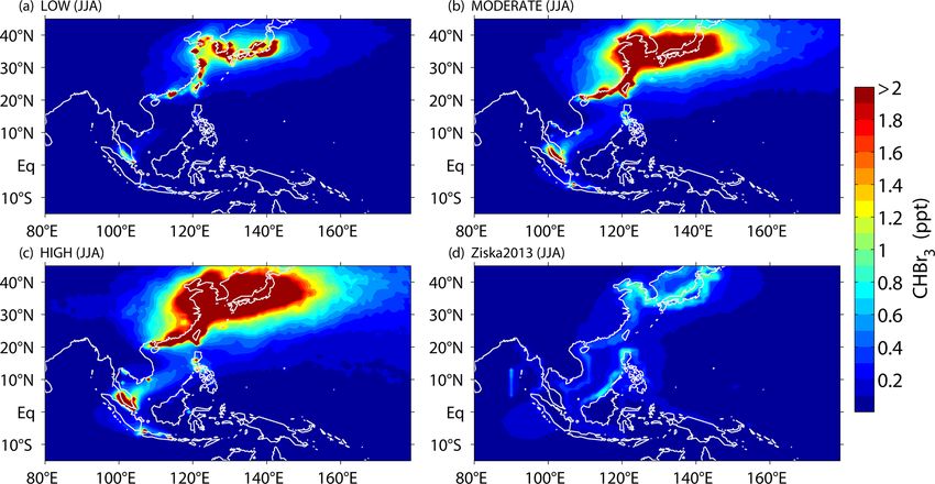
J. Maas et al.: Simulations of anthropogenic bromoform indicate high emissions at the coast of East Asia                   4105

ments cannot distinguish between naturally and industrially      2     Methods
produced bromoform, and all the top-down and bottom-up
emission estimates discussed above potentially include the       2.1    Estimation of DBP production in cooling water
latter already. A first comparison of natural and industrial            from East Asian power plants
bromoform sources from Quack and Wallace (2003) con-
cluded a negligible global contribution of 3 % man-made          In this study, we investigate the oceanic distribution of DBPs
bromoform. Their estimate was based on measurements of           produced in power plants that chlorinate seawater. We as-
bromoform in disinfected water (80 nmol L−1 ) from Euro-         sume that all power plants located at the coast use seawa-
pean power plants and cooling-water use and projections of       ter for cooling purposes. Most of the seawater is only used
the global electricity production. In the meantime, the global   once in the system as the ocean provides an unlimited wa-
electricity production has increased by almost 50 % from         ter supply. For the estimation of the cooling-water volumes,
16 700 TWh in 2003 (IEA, 2005) to 25 000 TWh in 2016             we use the global power plant database Enipedia from 2007
(IEA, 2018). Furthermore, new measurements of bromoform          (Davis, 2012; Davis et al., 2012), where over 21 000 power
in disinfected cooling water have become available, suggest-     plants are given together with location, electricity genera-
ing potentially higher concentrations of up to 500 nmol L−1      tion (in MWh) and sometimes fuel type. Based on the co-
(Padhi et al., 2012; Rajamohan et al., 2007; Yang, 2001).        ordinates, we choose those power plants that are located less
Emerging economies in East Asia, such as China and India,        than 0.02◦ (maximum 2 km at the Equator) away from any
have experienced a massive growth over the last years, ex-       coastline and refer to them as coastal. Based on this classifi-
ceeding the global economic growth. As the existing estimate     cation, 23 % of energy capacity from listed power plants in
of industrially produced bromoform is outdated, updated es-      the database is generated by coastal power plants. The Key
timates taking into account new measurements are required        World Energy Statistics (IEA, 2018) give a total global elec-
to assess the impact of anthropogenic activities on the pro-     tricity production of 24 973 TWh in 2016. The average water
duction and release of brominated VSLSs as well as their         use per MWh of energy was given by Taylor (2006) to be
contribution to stratospheric ozone depletion.                   144 m3 MWh−1 , which leads to a global cooling-water dis-
   We will derive a new bottom-up VSLS emission estimate         charge of about 800 billion m3 a−1 along the coast in 2016.
for East and Southeast Asia by quantifying anthropogenic         For the individual coastal power plants in East and Southeast
contributions to bromoform production. We will use avail-        Asia, annual cooling-water volumes are shown in Fig. 1.
able cooling-water measurements to predict oceanic and at-          To determine the amount of bromoform produced in the
mospheric bromoform concentrations in regions of exten-          cooling water, there are only a few measurements available
sive industrial activities. Based on comparisons to available    and the locations are limited (Table 1). Most data originate
ocean surface and atmosphere measurements, we will eval-         from several power plants in Europe (Allonier et al., 1999;
uate our predictions and discuss implications for an atmo-       Boudjellaba et al., 2016; Jenner et al., 1997), and some stud-
spheric bromine budget as well as future research needs. As      ies are based on measurements from single power plants
50 % of the global coastal cooling water is produced in East     in Asia (Padhi et al., 2012; Rajamohan et al., 2007; Yang,
and Southeast Asia, we define these areas as our study re-       2001). Only Yang (2001) provides DBP measurements in
gion. We identify locations of high industrial activity along    East Asia. Furthermore, the location where water is sampled
the coast of East and Southeast Asia and derive estimates        is not consistent among the different studies. Some samples
of released cooling water and therein contained bromoform        were taken in the coastal surface water at the power plant out-
(Sect. 2). Based on Lagrangian simulations in the ocean, we      let (Fogelqvist and Krysell, 1991; Yang, 2001), while other
derive the general marine distribution of non-volatile DBPs      studies sampled directly inside the power plant before dilu-
released with cooling water. For the case study of bromo-        tion with the ocean (Jenner et al., 1997; Rajamohan et al.,
form, we show oceanic distributions of the volatile DBP by       2007). The measurements show a very large variability rang-
taking air–sea exchange into account (Sect. 3). Based on         ing from 8–290 µg L−1 . As there is no systematic difference
the oceanic emissions, the atmospheric distribution of bro-      between measurements inside the power plant and at the
moform generated in industrial cooling water is simulated        power plant outlet, both types of measurements are given in
with a Lagrangian particle dispersion model (Sect. 4). Re-       Table 1 together in the first column.
sults are discussed and compared to existing observational          In addition to the sampling location, differences in the con-
atmospheric and oceanic distributions (Sect. 5). Methods are     centrations can result from water temperature, salinity and
described in Sect. 2, while conclusion and summary are pro-      dissolved organic carbon content, which vary with season.
vided in Sect. 6.                                                Colder water from mid- to high latitudes during winter re-
                                                                 quires less water treatment as the growth of pathogens takes
                                                                 longer compared to warm tropical or subtropical waters. The
                                                                 chlorination dosage and frequency of treatment also play a
                                                                 distinct role for the resulting DBP concentrations (Joint Re-
                                                                 search Council, 2001).

https://doi.org/10.5194/acp-21-4103-2021                                          Atmos. Chem. Phys., 21, 4103–4121, 2021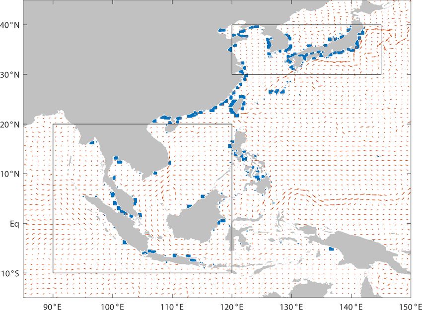
4106            J. Maas et al.: Simulations of anthropogenic bromoform indicate high emissions at the coast of East Asia

Figure 1. Location and annual cooling-water volume [billion m3 a−1 ] of coastal power plants in East and Southeast Asia extracted from the
Enipedia database and colour-coded by the cooling-water discharge.

Table 1. Bromoform concentrations measured in water samples from power plant cooling water and surrounding waters. Measurements in
the power plant effluent can refer to both samples of the undiluted water stream or seawater samples at the outlet.

         Power plant effluent/      Surroundings        Location                                   Reference
             near outlet         µg L−1 nmol L−1
         µg L−1    nmol L−1
         90–100      356–396        1–20        4–79    Gothenburg, Sweden, Kattegatt              Fogelqvist and Krysell (1991)
         9–17          35–67       0.1–5      0.4–20    North Sea                                  Jenner et al. (1997)
         8–27         32–107          n/a         n/a   English Channel                            Allonier et al. (1999)
         124             495        1–50       4–200    Youngkwang, South Korea, Yellow Sea        Yang (2001)
         20–290      79–1147        0–54       0–214    Kalpakkam, India, Bay of Bengal            Rajamohan et al. (2007)
         12–41        47–162          n/a         n/a   Kalpakkam, India, Bay of Bengal            Padhi et al. (2012)
         19               75     0.5–2.2         2–9    Gulf of Fos, France, Mediterranean         Boudjellaba et al. (2016)

   Given that available measurements are sparse and depend             and emission of the volatile DBP bromoform in the ocean.
on many factors, the uncertainties in initial bromoform con-           The Lagrangian model runs are based on velocity output
centrations in cooling water are relatively high. For our anal-        from the high-resolution, eddy-rich ocean general circulation
yses we chose to scale the bromoform discharge according               model (OGCM) NEMO-ORCA version 3.6 (Madec, 2008).
to three scenarios (LOW, MODERATE and HIGH), which                     The ORCA0083 configuration (The DRAKKAR Group,
reflect the range of values given in available literature (Ta-         2007) has a horizontal resolution of 1/12◦ at 75 vertical lev-
ble 1). For our simulations, we use initial bromoform con-             els, and output is given at a temporal resolution of 5 d for the
centrations of 20 µg L−1 (LOW), 60 µg L−1 (MODERATE)                   time period 1963–2012. Atmospheric forcing comes from
and 100 µg L−1 (HIGH) in undiluted cooling water.                      the DFS5.2 data set (Dussin et al., 2016). The experiment
                                                                       ORCA0083-N06 used in this study was run by the National
2.2    Lagrangian simulations in the ocean                             Oceanography Centre, Southampton, UK. Further details can
                                                                       be found in Moat et al. (2016).
To assess the long-term, large-scale effect of DBPs from                  We simulate the spread of the DBPs from treated cool-
power plant cooling water on the environment, we simulate              ing water by applying a Lagrangian trajectory integration
the distribution of non-volatile DBPs and the concentration

Atmos. Chem. Phys., 21, 4103–4121, 2021                                                   https://doi.org/10.5194/acp-21-4103-2021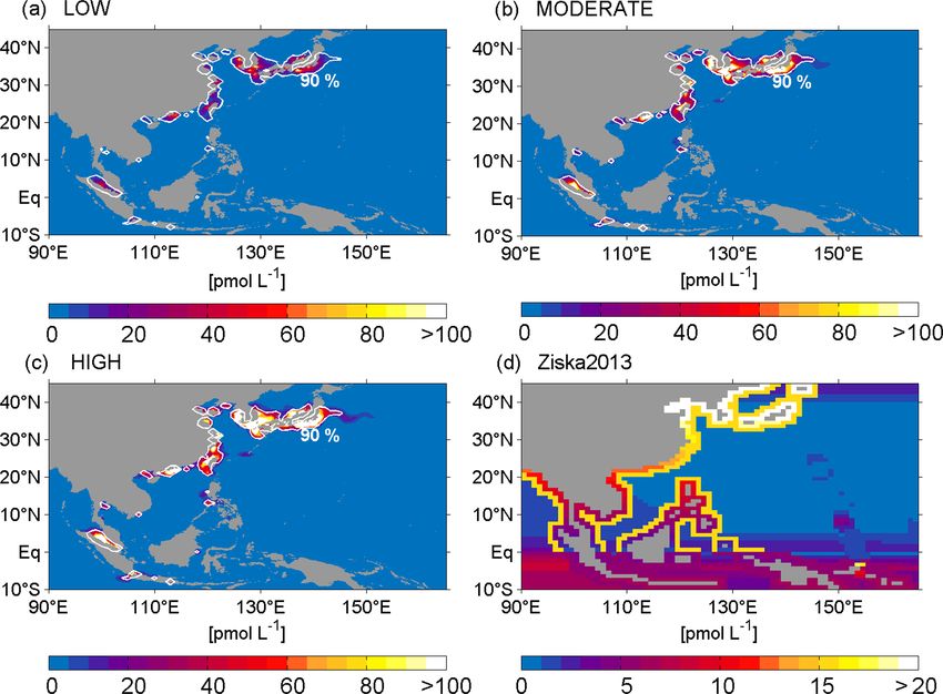
J. Maas et al.: Simulations of anthropogenic bromoform indicate high emissions at the coast of East Asia                           4107

Figure 2. Initial position of particles in East and Southeast Asia (blue dots). NEMO-ORCA0083 ocean currents from the initialisation time
in January 2005 (red arrows); the two boxes mark the regions referred to as tropics and subtropics as described in Sect. 2.3.

scheme to the 3D velocity fields with the Ariane software                 We conduct two different simulations allowing us to anal-
(Blanke et al., 1999). We perform offline trajectory calcula-          yse the spread of long-lived DBPs in general and the spread
tions by passively advecting virtual particles, which repre-           of bromoform as a specific case. First, we simulate the spread
sent the DBP amount discharged with the cooling water. The             of a passive tracer, which does not have any environmental
calculation of trajectories with Ariane is primarily based on          sinks and is representative of long-lived non-volatile DBPs.
advection. For each scenario we perform one simulation over            We consider the full history of simulated particle positions
the same time period from 2005/2006. The year chosen is the            which is equivalent to assuming no particles getting lost
same as in Maas et al. (2019), where it is shown that inter-           through sinks in the ocean or emission into the atmosphere.
annual variability of surface velocity in the study region is          The resulting distribution shows locations where non-volatile
small compared to seasonal variability. In each simulation,            DBPs such as bromoacetic acid are transported through the
particles are continuously released close to the power plant           ocean currents within 1 year.
locations at 5 d time steps over 2 years. We allow for an ac-             Second, we simulate the spread of bromoform as a major
cumulation period of 11 months and show the results of the             volatile DBP including the simulation of atmospheric fluxes
seasonal and annual mean of the second year starting in De-            and oceanic sinks. Each particle is assigned an initial mass of
cember 2005. A detailed description of the applied method              bromoform according to the amount of cooling water used by
can be found in Maas et al. (2019).                                    the respective power plant (Fig. 1) and the bromoform con-
   Our study focusses on the region of East and Southeast              centration prescribed by the three scenarios: MODERATE,
Asia (90–165◦ E, 10◦ S–45◦ N), which comprises 50 % of the             HIGH and LOW. The particle density distribution is calcu-
global coastal power plant capacity and cooling-water dis-             lated at the sea surface down to 20 m on a 1◦ × 1◦ grid. The
charge. The particle discharge locations have been chosen              distribution is given as particle density per grid box in per-
as close to the coastlines as possible (Fig. 2). Particles are         cent for non-volatile DBPs and as concentration in pmol L−1
released approximately 8 to 40 km offshore, as the model-              for bromoform.
resolution does not allow us to capture smaller-scale coastal             For the second set of simulations, the sink processes of
structures such as harbours or estuaries, nor does it simulate         bromoform such as constant gas exchange at the air–sea in-
the near-costal exchange, e.g. through tides. Our approach             terface or chemical loss rates are taken into account. The
ensures minimal influence of the land boundaries on the sim-           air–sea flux of bromoform is calculated following the gen-
ulation in order to avoid numerically related beaching of par-         eral flux equation at the air–sea interface:
ticles into the coastal boundary.
                                                                       Flux = (Cw − Ceq ) × k.                                       (1)

https://doi.org/10.5194/acp-21-4103-2021                                                 Atmos. Chem. Phys., 21, 4103–4121, 2021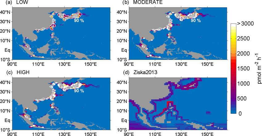
4108           J. Maas et al.: Simulations of anthropogenic bromoform indicate high emissions at the coast of East Asia

Here flux is positive when it is directed from the ocean to the   moist convection (Forster et al., 2007) and turbulence in the
atmosphere and is given in pmol m−2 h−1 . Cw is the actual        boundary layer and free troposphere (Stohl and Thomson,
concentration in the surface mixed layer in pmol L−1 , and        1999). It has been used in previous studies with a similar
              −1
                                                                  model set-up and shown robust VSLS profiles compared to
Ceq = Cair × HCHBr 3
                                                           (2)    observations (e.g. Fiehn et al., 2017; Fuhlbrügge et al., 2016;
is the theoretical equilibrium concentration at the sea surface   Tegtmeier et al., 2020a).
(in pmol L−1 ) calculated from the atmospheric mixing ratio          Seasonal mean bromoform emissions derived from the
(in ppt) and Henry’s law constant HCHBr3 of bromoform. The        three scenarios are used as input data at the air–sea interface
gas transfer velocity k (in cm h−1 ) mainly depends on the        over the East and Southeast Asia area defined as our study re-
surface wind speed and temperature and is calculated follow-      gion. The meteorological input data (temperature and winds)
ing Nightingale et al. (2000). Wind velocities at 10 m height     stem from the ERA-Interim reanalysis product (Dee et al.,
are taken from the NEMO-ORCA forcing data set DFS5.2              2011) and are given on a 1◦ ×1◦ horizontal grid, at 61 vertical
(Dussin et al., 2016), which is based on the ERA-Interim at-      model levels and a 3-hourly temporal resolution. The chem-
mospheric data product.                                           ical decay of bromoform in the atmosphere was accounted
   As the oceanic and atmospheric terms in the air–sea flux       for by prescribing a lifetime of 17 d during all runs (Montzka
parameterisation are of additive nature, it is possible to cal-   and Reimann, 2010).
culate the flux of anthropogenic and natural bromoform sep-          The FLEXPART simulations were performed for bo-
arately. For our simulations, we only consider bromoform          real winter (December–February, DJF) and summer (June–
from cooling water and apply the air–sea flux parameterisa-       August, JJA) seasons, respectively, each with a 2-month spin-
tion to the anthropogenic portion of bromoform in water and       up phase. Since there are only weak dynamical variations be-
air. We have conducted sensitivity tests (see Sect. 2.3) to es-   tween different years, we used an ensemble mean of 4 years
timate the impact that atmospheric bromoform abundances           (2015–2018) each. A total of 1000 particles are randomly
have upon the flux calculations. The tests show that out-         seeded inside each grid box at each time step according to
gassed anthropogenic bromoform leads to atmospheric sur-          the air–sea flux strength. Output mixing ratios are given at
face values Ceq , which are always below 8 % of the underly-      the same horizontal resolution and 33 vertical levels from
ing sea surface concentration Cw (at a water temperature of       50 to 20 000 m. Detailed descriptions of model settings are
20 ◦ C). Such low equilibrium concentrations can be consid-       described in Jia et al. (2019).
ered negligible for the flux calculation, and therefore Ceq is       We perform three additional FLEXPART runs, Ziska2013-
set to zero in our study.                                         EastAsia, Ziska2013 and Ziska2013 + MODERATE, based
   The sea surface concentration and air–sea flux from the        on the updated Ziska2013 emission inventory with the same
three simulations are also compared to climatological maps        FLEXPART configuration as described above for both sea-
of bromoform concentration and emissions from the up-             sons, DJF and JJA. As the Ziska2013 inventory currently
dated Ziska et al. (2013) inventory (hereafter referred to as     presents our best knowledge of bottom-up bromoform emis-
Ziska2013) (Fiehn et al., 2018a).                                 sions, it is of interest to analyse how much of these emissions
   Mean sea surface concentrations Cw are calculated by av-       can be explained by industrial sources and how much stems
eraging over the area where 90 % of all released bromoform        from natural sources.
accumulates. To this end, all grid cells are sorted according        The Ziska2013-EastAsia run uses only the Ziska2013 cli-
to descending bromoform concentrations and the average is         matological emissions over East and Southeast Asia defined
calculated over the first grid cells that contain in total 90 %   as our study region. Results from Ziska2013-EastAsia in the
of all bromoform. Maximum concentrations are calculated           atmospheric boundary layer are used to compare the mixing
by averaging over the area where 10 % of the highest bromo-       ratios based on our anthropogenic emissions in the East and
form values accumulate. Mean and maximum air–sea fluxes           Southeast Asia region.
are calculated using the same averaging principle as for Cw .        For comparisons of mixing ratios in the free troposphere
The annual mean atmospheric bromine flux resulting from           and upper troposphere–lower stratosphere (UTLS), air–sea
industrial bromoform emissions in East and Southeast Asia         fluxes from other parts of the tropics also need to be taken
is derived from the air–sea flux maps of the whole domain.        into account as the timescales for horizontal transport are of-
                                                                  ten shorter than the ones for vertical transport. Therefore, we
2.3    Lagrangian simulation in the atmosphere                    set up the runs Ziska2013 and Ziska2013 + MODERATE.
                                                                  Ziska2013 uses the air–sea flux of the Ziska2013 clima-
Based on the seasonal mean emission maps, we obtain a             tology for the global tropics and subtropics between 45◦ S
source function of atmospheric bromoform. We simulate             and 45◦ N. As the Ziska2013 climatology is taking into
the atmospheric transport and distribution of bromoform for       account only very few northern hemispheric coastal data
the three different emission strength scenarios with the La-      points, it likely neglects anthropogenic fluxes in some re-
grangian particle dispersion model FLEXPART (Stohl et al.,        gions. Therefore, the Ziska2013 + MODERATE run uses the
2005). The FLEXPART model includes parameterisation for           Ziska2013 fluxes between 45◦ S and 45◦ N but replaces them

Atmos. Chem. Phys., 21, 4103–4121, 2021                                            https://doi.org/10.5194/acp-21-4103-2021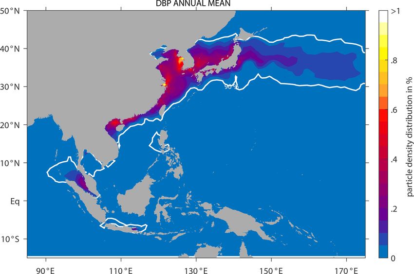
J. Maas et al.: Simulations of anthropogenic bromoform indicate high emissions at the coast of East Asia                             4109

Figure 3. Annual mean particle density distribution in percent (%) of DBPs from cooling-water treatment in coastal power plants in East and
Southeast Asia. The white contour line shows the patches where 90 % of the largest particle density is located.

with the anthropogenic MODERATE flux values in all grid                 distribution south of 20◦ N, except for higher values in the
boxes where the MODERATE fluxes are larger than the                     Strait of Malacca. In contrast to the relatively low DBP den-
Ziska2013 fluxes. The two runs, Ziska2013 + MODERATE                    sity in the inner tropics, the subtropics show a very high ac-
and Ziska2013, are used to quantify the additional anthro-              cumulation of DBPs with a centre in the marginal seas be-
pogenic bromoform based on the MODERATE scenario in                     tween 25 and 40◦ N. While power plants can be found along
the UTLS region. The UTLS region is calculated as the                   all coastlines (Fig. 1), the power plant capacity and therefore
height of the cold-point tropopause, which has been derived             the amount of treated cooling water is much higher along
from ERA-Interim model level data at 6-hourly resolution                the subtropical coasts of China, Korea and Japan, leading to
(Tegtmeier et al., 2020b).                                              the DBP distribution pattern shown in Fig. 3. Hotspots are
   Mean mixing ratios from the whole domain (90–165◦ E,                 around the coast of Shanghai and Incheon, with a DBP den-
10 S–45◦ N) in the marine boundary layer and in the UTLS
   ◦                                                                    sity of 1 %. A relatively high DBP density of 0.8 % can also
are given as the average over the 90 % area characterised               be found in the East China Sea, the Yellow Sea, the southern
by the highest local values, and maximum mixing ratios are              Sea of Japan, the Gulf of Tonkin and the Strait of Malacca.
given as the average over the largest 10 % (see Sect. 2.2). In          Medium to low DBP density in the South China Sea sug-
a second step, we define two regions in order to analyse the            gests only small contributions of cooling waters to this re-
vertical transport of bromoform into the free troposphere and           gion. Since Japan and Korea have a large number of power
into the UTLS. For the height profiles of the Ziska2013 and             plants with high volumes of cooling-water discharge, a rela-
the Ziska2013 + MODERATE runs, we average mixing ra-                    tively large amount of DBPs is transported eastward with the
tios over a region above the Maritime Continent, which we               Kuroshio Current east of Japan into the North Pacific.
refer to as the tropical box (10◦ S–20◦ N, 90–120◦ E), and                 The distribution of bromoform as a volatile DBP in the sur-
over another region from China to Japan, which we refer to              face ocean differs from the DBP accumulation pattern shown
as the subtropical box (30–40◦ N, 120–145◦ E) (Fig. 2).                 in Fig. 3, because the volatile DBPs are outgassed into the
                                                                        atmosphere. The annual mean sea surface concentration of
                                                                        bromoform from cooling water is shown in Fig. 4a–c for
                                                                        the three cooling-water discharge scenarios LOW, MODER-
3   Oceanic spread of DBPs and bromoform
                                                                        ATE and HIGH and with a substantially smaller spread com-
The particle density distribution shows the annual mean DBP             pared to the non-volatile DBPs. The area which contains the
accumulation pattern in the region of interest in East and              90 % highest bromoform concentrations does not vary be-
Southeast Asia (Fig. 3). Non-volatile DBPs from cooling wa-             tween the three scenarios, as the air–sea flux, which deter-
ter usually accumulate around the coast and in the marginal             mines how much bromoform remains in the water, is linearly
seas. There is a clear latitudinal gradient with only little DBP        proportional to the sea surface concentration. Higher surface

https://doi.org/10.5194/acp-21-4103-2021                                                  Atmos. Chem. Phys., 21, 4103–4121, 2021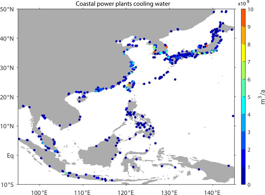
4110           J. Maas et al.: Simulations of anthropogenic bromoform indicate high emissions at the coast of East Asia

Figure 4. Annual mean surface bromoform concentration in pmol L−1 for the three scenarios (a) LOW, (b) MODERATE and (c) HIGH
as well as (d) the bromoform surface map updated from Ziska2013. Note that the colour bar limits for panel (d) vary from the limits in
panels (a)–(c). The white contour line in panels (a)–(c) shows the patches where 90 % of the largest concentrations are located.

concentrations result in higher fluxes into the atmosphere,          mum lies around 21 pmol L−1 . Our simulations reach max-
which limits the spread of bromoform substantially com-              imum values (averaged over the 10 % highest bromoform
pared to non-volatile DBPs. Bromoform concentrations are             concentrations) of 112, 338 and up to 563 pmol L−1 (LOW,
around 23, 68 and 113 pmol L−1 (LOW, MODERATE and                    MODERATE and HIGH, Table 2) in the Sea of Japan. These
HIGH), averaged over the region where the 90 % of bromo-             concentrations are all above 100 pmol L−1 and are very high
form with the highest concentrations accumulates (Table 2).          compared to observational values from Ziska2013 (Fig. 4d).
This region is to a large degree limited to latitudes north of          Air–sea fluxes of anthropogenic bromoform show a sim-
20◦ N as a result of the power plant distribution. As in the         ilar distribution as the oceanic concentrations (Fig. 5a–c).
case of the non-volatile DBPs, most of the bromoform is cen-         Flux rates averaged over the region of the 90 % highest flux
tred along the Chinese, Korean and Japanese coastline, with          values are 3, 9 and 15 nmol m−2 h−1 (LOW, MODERATE
a larger spread into the marginal seas for the latter two. One       and HIGH). Maximum flux rates (averaged over the highest
exception to this latitudinal gradient is the Strait of Malacca,     10 %) even reach 13, 41 and 68 nmol m−2 h−1 in the Sea of
where local power plants result in average bromoform con-            Japan near the Korean and Japanese coast for the three sce-
centrations of 3.4, 10.3 and 16.7 pmol L−1 (LOW, MODER-              narios (Table 2). In contrast, the existing observation-based
ATE, and HIGH).                                                      estimates from the Ziska2013 climatology peak with a flux
   Observation-based oceanic bromoform concentrations                of 1.1 nmol m−2 h−1 in the South China Sea along the west
from Ziska2013 (Fig. 4d) are relatively evenly spread along          coast of the Philippines (Fig. 5d).
the coastlines of the region and do not show the latitudinal            The annual bromine input from the ocean into the at-
gradient found for the anthropogenic concentrations. North           mosphere in the form of bromoform emissions in the East
of 20◦ N the anthropogenic bromoform is much higher than             and Southeast Asia region is 118 Mmol of Br according to
the oceanic distribution from Ziska2013, where the maxi-             the observation-based inventories from Ziska2013 (Table 2).

Atmos. Chem. Phys., 21, 4103–4121, 2021                                                https://doi.org/10.5194/acp-21-4103-2021

J. Maas et al.: Simulations of anthropogenic bromoform indicate high emissions at the coast of East Asia                                   4111

Table 2. Mean and maximum bromoform concentration [pmol L−1 ] for the three Ariane runs LOW, MODERATE, and HIGH, as well as the
climatological values from the Ziska2013 bottom-up estimate in East and Southeast Asia. Mean and maximum air–sea flux [pmol m−2 h−1 ]
from the three scenarios and the Ziska2013 air–sea flux in East and Southeast Asia. The annual mean bromine flux [Mmol Br a−1 ] is derived
from the air–sea flux of the total domain in East and Southeast Asia. Mean and maximum atmospheric bromoform mixing ratios in the marine
boundary layer [ppt] from the four FLEXPART runs. Values are given as the mean and the standard deviation averaged over the largest 90 %
(referred to as mean values) and over the largest 10 % (referred to as maximum values).

 Scenario             Sea surface concentration         Air–sea flux          Bromine flux         Atmospheric CHBr3 mixing ratio [ppt]
                             [pmol L−1 ]              [pmol m−2 h−1 ]        [Mmol Br a−1 ]           JJA                     DJF
                          Mean             Max         Mean          Max         Total          Mean          Max     Mean              Max
 LOW                    23 ± 24    112.1 ± 6.3      3.1 ± 3.4   13.7 ± 0.9        100          0.4 ± 0.9    9.0 ± 1.3   0.3 ± 0.5     4.7 ± 2.6
 MODERATE               68 ± 74   338.3 ± 16.6     9.1 ± 10.2   41.1 ± 2.9        300          1.3 ± 2.7   27.1 ± 3.5   0.8 ± 1.4    13.5 ± 7.7
 HIGH                 113 ± 122   563.6 ± 28.8    15.1 ± 16.9   68.5 ± 4.7        500          2.2 ± 4.4   45.0 ± 6.3   1.4 ± 2.4   23.3 ± 12.9
 Ziska2013-EastAsia       7±6       21.3 ± 1.3      0.4 ± 0.2    1.1 ± 0.2        118          0.2 ± 0.1    0.8 ± 0.2   0.2 ± 0.1     0.5 ± 0.1

Figure 5. Annual mean air–sea flux of bromoform in pmol m−2 h−1 for the three scenarios (a) LOW, (b) MODERATE, and (c) HIGH, as well
as (d) the air–sea flux calculated from updated ocean and atmospheric maps following Ziska2013. The white contour line in panels (a)–(c)
shows the patches where 90 % of the largest emissions are located.

Our simulations suggest that the anthropogenic input alone               is released over 1 year, compared to the tropical Southeast
amounts to 100, 300 and 500 Mmol Br a−1 (LOW, MODER-                     Asian regions south of 20◦ N where only 10–52 Mmol Br a−1
ATE and HIGH) for the same region, which corresponds to                  enters the atmosphere (from LOW to HIGH). In contrast,
almost 99 % of the bromine produced during cooling-water                 only 29 % of the total bromine from the Ziska2013 clima-
treatment in the power plant for each scenario. This implies             tology in East Asia is released into the atmosphere north of
that all bromoform from cooling-water treatment is eventu-               20◦ N, which suggests that the majority of the anthropogenic
ally outgassed from the ocean into the atmosphere. While                 emissions from this region are missing in the Ziska2013 cli-
average and maximum air–sea fluxes of anthropogenic bro-                 matology.
moform are much higher and confined to small areas around
the discharge locations, the Ziska2013 air–sea fluxes are dis-
tributed along all coastlines and along the Equator and result
in a similar total annual mean Br flux as the LOW emission
scenario (Table 2). A total of 90 % of the annual mean at-
mospheric bromine input from anthropogenic bromoform in
East Asia occurs north of 20◦ N where 89–447 Mmol of Br

https://doi.org/10.5194/acp-21-4103-2021                                                      Atmos. Chem. Phys., 21, 4103–4121, 2021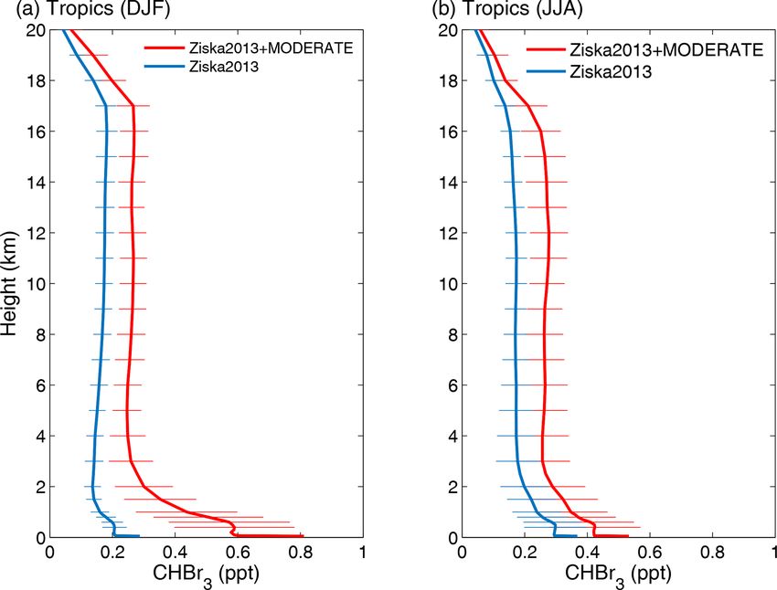
4112 J. Maas et al.: Simulations of anthropogenic bromoform indicate high emissions at the coast of East Asia
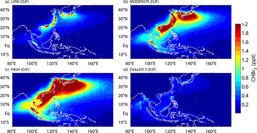
Figure 6. Seasonal mean bromoform mixing ratios [ppt] in 50 m height during JJA derived from FLEXPART runs driven by the three
scenarios (a) LOW, (b) MODERATE, (c) HIGH, and (d) Ziska2013-EastAsia.
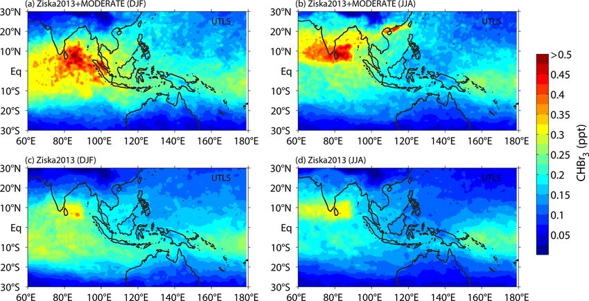
4 Anthropogenic bromoform in the atmosphere In contrast to boreal summer, the atmospheric transport is
dominated by winds from the northeast, and higher bromo-
4.1 Mixing ratios in the marine boundary layer form values are confined to tropical and subtropical regions
(Fig. 7). Thus, tropical mixing ratios show a clear seasonal
variability and are on average over 3 times higher for DJF
Atmospheric mixing ratios of anthropogenic bromoform are than for JJA without large shifts in the location of the bromo-
derived from FLEXPART runs driven by the seasonal emis- form emissions (Fig. S1 in the Supplement).
sion estimates discussed in Sect. 3. Atmospheric bromoform In order to compare the atmospheric impact of indus-
from industrial emissions is shown for a seasonal average trial emissions with existing results, we repeat our analy-
in the marine boundary layer at 50 m height for JJA for all sis for the bottom-up emissions scenario Ziska2013 for the
three scenarios (Fig. 6a–c). Mean mixing ratios are 0.4, 1.3 same region, which has been frequently used in past stud-
and 2.3 ppt (LOW, MODERATE and HIGH, Table 2). Over- ies (e.g. Hossaini et al., 2013, 2016). Atmospheric mixing
all, high atmospheric mixing ratios are found around the ratios are derived from seasonal FLEXPART runs driven
coastlines of Japan, South Korea and northern China. Al- by Ziska2013-EastAsia and shown for a seasonal average
though maximum emissions are located in the Sea of Japan, at 50 m height for JJA (Fig. 6d). For both seasons, JJA
maximum mixing ratios are mostly located south of Japan and DJF, atmospheric bromoform based on industrial emis-
with values up to 9.0, 27.1 and 45.0 ppt (LOW, MODERATE sions is larger than atmospheric bromoform based on the
and HIGH, Table 2). Here, the westerlies lead to bromoform Ziska2013-EastAsia emissions (Figs. 6d and 7d). These dif-
transport from the Sea of Japan into the northwest Pacific. We ferences are maximised in the subtropical regions, where
also localise hotspots of strong anthropogenic bromoform ac- anthropogenic bromoform dominates especially during JJA
cumulations due to enhanced emissions over Shanghai, Sin- when anthropogenic mixing ratios are 2–5 times larger com-
gapore or the Pearl River Delta, respectively (Fig. 6a). Dur- pared to climatological Ziska2013 bromoform (for LOW and
ing boreal summer, the western Pacific and Maritime Conti- MODERATE). In the tropical regions, the situation is more
nent are influenced by southwesterly winds, and the anthro- complicated. Atmospheric abundances driven by the indus-
pogenic bromoform experiences northward transport, bring- trial emissions reach higher peak values of up to 2 ppt, espe-
ing some smaller portion of the subtropical emissions into cially in the Strait of Malacca (MODERATE, Fig. 6b), while
the mid-latitudes (Fig. 6a–c). mixing ratios driven by the observationally based emissions
During boreal winter (DJF, Fig. 7a–c), anthropogenic bro- from Ziska2013-EastAsia are smaller, only reaching peak
moform shows somewhat lower atmospheric mixing ratios values of up to 0.8 ppt, but are spread over a much wider
with a mean of 0.3, 0.8 and 1.4 ppt and maximum values area (Fig. 6d). Given the comparison of the boundary layer
of 4.7, 13.5 and 23.3 ppt for the three scenarios (Table 2).
Atmos. Chem. Phys., 21, 4103–4121, 2021 https://doi.org/10.5194/acp-21-4103-2021J. Maas et al.: Simulations of anthropogenic bromoform indicate high emissions at the coast of East Asia 4113 Figure 7. Same as Fig. 6 only during DJF. values, it is not clear which emission scenario will result in a larger contribution to the stratospheric halogen budget. 4.2 Mixing ratios in the free troposphere and UTLS In order to analyse atmospheric transport from the marine boundary layer into the free troposphere and UTLS, sea- sonal mean bromoform mixing rations are averaged over a subtropical box (30–40◦ N, 120–145◦ E, Fig. 2) and a tropical box (10◦ S–20◦ N, 90–120◦ E, Fig. 2) from the Ziska2013 and Ziska2013 + MODERATE simulations for DJF and JJA. Both simulations are based on global climato- logical Ziska2013 bromoform air–sea fluxes between 45◦ S and 45◦ N, with Ziska2013 + MODERATE including addi- tional anthropogenic bromoform fluxes in East and Southeast Asia. In the subtropical box (Fig. 8), there is a strong domi- Figure 8. Height profile of seasonal mean bromoform mixing ratio nance of anthropogenic bromoform in the marine boundary [ppt] in the subtropics (30–40◦ N, 120–145◦ E) during JJA for the layer during JJA that is several times higher compared to bro- Ziska2013 + MODERATE run (red) and the Ziska2013 run (blue). moform from climatological bottom-up emissions (Fig. 8). Additionally shown is the averaged profile of bromoform measure- Our simulations suggest that during convective events in ments from the KORUS-AQ campaign over South Korea and the JJA, anthropogenic bromoform from the subtropical ma- Yellow Sea (black). Horizontal lines show the standard deviation rine boundary layer can be transported into the UTLS re- for specific heights. gion, up to the height of the cold point. In our simula- tion Ziska2013 + MODERATE, convective events during the summer bring on average over 0.3 ppt into the UTLS (Fig. 8). Zone (ITCZ) is located north of 10◦ N (Waliser and Gautier, During DJF (not shown), there is only very little transport 1993). of bromoform out of the boundary layer, and entrainment of In the tropical box (Fig. 9), atmospheric bromoform mix- anthropogenic bromoform into the subtropical UTLS is con- ing ratios in the marine boundary layer are generally weaker fined to boreal summer when the Intertropical Convergence than in the subtropics (Fig. 8). The seasonal difference be- https://doi.org/10.5194/acp-21-4103-2021 Atmos. Chem. Phys., 21, 4103–4121, 2021
4114            J. Maas et al.: Simulations of anthropogenic bromoform indicate high emissions at the coast of East Asia

                                                                        In addition to the mixing ratios averaged over two boxes,
                                                                     we show the spatial distribution of seasonally averaged bro-
                                                                     moform mixing ratios at the cold-point tropopause for the
                                                                     whole domain (90–165◦ E, 10◦ S–45◦ N) (Fig. 10) based
                                                                     on the Ziska2013 and Ziska2013 + MODERATE emissions.
                                                                     During DJF (Fig. 10a and c), there is a clear anthropogenic
                                                                     signal over the Bay of Bengal, across the Equator towards
                                                                     Indonesia. Mixing ratios for the Ziska2013 + MODERATE
                                                                     run are 0.22 ± 0.07 ppt, averaged over the area of 90 % high-
                                                                     est mixing ratios, and 0.18 ± 0.05 ppt for Ziska2013, which
                                                                     implies that 0.04 ppt is of anthropogenic origin (Table S1 in
                                                                     the Supplement). Again, the strong advective transport in the
                                                                     boundary layer during DJF bringing higher bromoform abun-
                                                                     dances from the subtropics into the tropics plays an impor-
                                                                     tant role here. Some fraction of the advected bromoform is
                                                                     picked up by tropical deep convection and transported into
Figure 9. Height profile of seasonal mean bromoform mix-             the UTLS and up to the cold point. As the latter represents
ing ratio [ppt] in the tropics (10◦ S–20◦ N, 90–120◦ E) for the      the stratospheric injection level, the interaction of boundary
Ziska2013 + MODERATE run (red) and Ziska2013 run (blue) for          layer advection and local convection over the Indian Ocean
both (a) DJF and (b) JJA. Horizontal lines show the standard devi-   and Maritime Continent results in an efficient transport path-
ation for specific heights.
                                                                     way for anthropogenic bromoform from industrial sources in
                                                                     East Asia to the stratosphere.
                                                                        During JJA (Fig. 10b and d), mean bromoform mixing ra-
tween DJF and JJA is only pronounced in the tropical marine
                                                                     tios averaged over the area of 90 % highest mixing ratios are
boundary layer for Ziska2013 + MODERATE, where mix-
                                                                     slightly smaller, with 0.20 ± 0.06 and 0.15 ± 0.05 ppt based
ing ratios during DJF exceed 0.5 ppt throughout the whole
                                                                     on the Ziska2013 + MODERATE and Ziska2013 emissions,
time period (Fig. 9a) and are around 0.4 ppt during JJA
                                                                     respectively (Table S1). During the Asian summer monsoon,
(Fig. 9b). The air–sea fluxes show no strong seasonal vari-
                                                                     the region of main upward transport of VSLS lies at about
ations; therefore, this difference must be transport driven.
                                                                     20◦ N over the Indian Ocean so that the main stratospheric
During DJF, the prevailing northeasterly winds advect the
                                                                     injection region of VSLSs shifts to the Bay of Bengal and
bromoform from regions of high anthropogenic emissions
                                                                     northern India (Fiehn et al., 2018b). However, most of the
in East Asia towards the Maritime Continent, increasing the
                                                                     boundary layer bromoform from anthropogenic sources stays
tropical bromoform abundance substantially. Thus, tropical
                                                                     in the Northern Hemisphere around the coastline of China
convection during DJF can transport more of the anthro-
                                                                     and over the western Pacific, thus decoupled from the mon-
pogenic bromoform emitted in East Asia into the UTLS com-
                                                                     soon convection.
pared to similar events during JJA (Fig. 9). The difference be-
                                                                        While over 90 % of anthropogenic bromoform is out-
tween the Ziska2013 + MODERATE and the Ziska2013 av-
                                                                     gassed north of 20◦ N, our simulations show that the ad-
erage mixing ratios in the UTLS is 0.05 ppt during DJF and
                                                                     ditional anthropogenic emissions in the MODERATE sce-
0.04 ppt during JJA. These values present the anthropogenic
                                                                     nario contribute on average 0.05 ppt of CHBr3 during JJA to
contribution to stratospheric bromine from East and South-
                                                                     0.04 ppt of CHBr3 during DJF to the stratospheric bromine
east Asian cooling water based on the MODERATE bromo-
                                                                     budget at the UTLS (Table S1). This is an increase of 22 %–
form emission scenario.
                                                                     32 % compared to the Ziska2013 mixing ratios of 0.15 and
   Atmospheric processes over the Maritime Continent,
                                                                     0.18 ppt of CHBr3 during JJA and DJF, respectively.
which encloses the tropical box, are characterised by
deep convective events, which can lead to entrainment of
VSLSs into the stratosphere (Aschmann and Sinnhuber,
2013; Tegtmeier et al., 2020a). For our case study, con-             5     Discussion
vective events reaching the UTLS occur in both seasons
(Fig. 9). Moreover, here is a clear anthropogenic signal from        5.1    Comparison with bromoform measurements in the
Ziska2013 + MODERATE compared to Ziska2013 in the                           ocean
free troposphere in this region in both seasons, which is more
                                                                     Observations of bromoform in the surface ocean and atmo-
pronounced during DJF (Fig. 9a) than during JJA (Fig. 9b),
                                                                     sphere from East and Southeast Asia can help to determine
in agreement with the elevated mixing ratios in the marine
                                                                     which scenario (LOW, MODERATE and HIGH) offers the
boundary layer.
                                                                     best fit for simulating anthropogenic bromoform in this re-
                                                                     gion. Recent measurement campaigns show elevated bromo-

Atmos. Chem. Phys., 21, 4103–4121, 2021                                                 https://doi.org/10.5194/acp-21-4103-2021
J. Maas et al.: Simulations of anthropogenic bromoform indicate high emissions at the coast of East Asia 4115 Figure 10. Seasonal mean atmospheric CHBr3 mixing ratios [ppt] for (a, b) the Ziska2013 + MODERATE and (c, d) the Ziska2013 simu- lation at the cold-point tropopause height for (a, c) DJF and (b, d) JJA. form concentrations in the coastal waters of the East China coast as observed by Yang (2001) and confirmed by our sim- and Yellow seas (He et al., 2013a, b; Yang et al., 2014, 2015). ulations. Our simulated anthropogenic bromoform concen- Average values of 6–13 pmol L−1 were measured in the Yel- trations stay usually within 100 km of the coast; the aver- low and East China seas during boreal spring and summer aged observational values, however, include also measure- (Yang et al., 2014, 2015), and 17 pmol L−1 was measured in ments that are up to 200 km away from the coastline and can boreal winter (He et al., 2013b). Particularly high concen- therefore be expected to be lower. While observational mean trations were detected by He et al. (2013a) during spring in values are slightly lower than our model results, maximum the East China Sea with a mean of 134 pmol L−1 . The high- values found close to the coastline show very good agree- est bromoform concentration over 34 pmol L−1 (He et al., ment with the model results. 2013b) and over 200 pmol L−1 (He et al., 2013a) was ob- served near the estuaries of the Yangtze River, which the au- 5.2 Comparison with bromoform measurements in the thors attributed to anthropogenic activities including coastal troposphere water treatment in the Shanghai region. Our simulations also show mean surface concentrations around Shanghai of 14– An extensive study of atmospheric measurements over 71 pmol L−1 (LOW to HIGH), in the range of the observa- South Korea and adjacent seas was performed in spring tions by He et al. (2013a). (May and June) 2016 by the Korea–United Sates Air Measurements in the South China and Sulu seas Quality Study (KORUS-AQ; https://www-air.larc.nasa.gov/ (Fuhlbrügge et al., 2016) show a high variability of bromo- missions/korus-aq/, last access: 1 March 2021). The aircraft form in the surface seawater with average concentrations of measurements of various VSLSs including bromoform were 19.9 pmol L−1 . The highest values of up to 136.9 pmol L−1 repeatedly taken between 0 and 12 km in the region between are found close to the Malaysian Peninsula and especially 30–40◦ N and 120–145◦ E, coinciding with our subtropical in the Singapore Strait, suggesting industrial contributions. box discussed earlier (Fig. S2). The data used here are based Maximum anthropogenic bromoform from our simulations on the 60 s merged data set from all flight sections. In the in the Singapore Strait ranges from 36–178 pmol L−1 (LOW campaign region around South Korea, an average bromoform to HIGH), in good agreement with maximum values reported atmospheric mixing ratio from all sections of 2.5 ± 1.4 ppt by Fuhlbrügge et al. (2016). was measured in the lower 100 m (Fig. 8). In comparison, Average anthropogenic bromoform concentrations for the our simulations for the Ziska2013 + MODERATE scenario three scenarios are around 23–113 pmol L−1 (averaged over show an average mixing ratio of 3.8 ± 1.4 ppt in the low- the region of the 90 % highest values, Table 2) and are larger est 100 m in the subtropical box during JJA. The simulations than the observational average values. The larger model val- based on Ziska2013 give a bromoform mixing ratio of only ues might be due to the fact that the cooling-water effluents 0.3 ± 0.1 ppt for the same altitude range, demonstrating that do not distribute far into the marginal seas but stay near the the additional anthropogenic bromoform results in a much https://doi.org/10.5194/acp-21-4103-2021 Atmos. Chem. Phys., 21, 4103–4121, 2021
4116           J. Maas et al.: Simulations of anthropogenic bromoform indicate high emissions at the coast of East Asia

better agreement with the observations in the marine bound-       5.3   Discussion of uncertainties
ary layer around South Korea.
   Above the boundary layer, mixing ratios from KORUS-            Our analyses suggests that anthropogenic bromoform accu-
AQ rapidly decline to 0.5–0.7 ppt in the 3–9 km altitude          mulates in the boundary layer, increasing the bromine budget
range (Fig. 8). Here, the Ziska2013 + MODERATE simu-              in East and Southeast Asia by 85 %–254 % compared to the
lation suggest seasonal mean mixing ratios between 0.4–           Ziska2013 climatology. This input can be expected to impact
0.7 ppt, which fit very well to the KORUS-AQ data. Sim-           tropospheric bromine budget and ozone chemistry. While we
ulations based on Ziska2013 suggest 0.2 ppt bromoform in          have not analysed these aspects in our study, it should be
this region, clearly underestimating the observations (Fig. 8).   investigated in follow-on projects. The highest uncertainties
Between 9 and 12 km, the observed bromoform values drop           in the estimates presented here arise from the highly vari-
sharply to values around 0.2 ± 0.08 ppt, suggesting that the      able bromoform amounts found in chemically treated cool-
aeroplane probed air masses above the convective outflow.         ing water. Since there are very few and no recent measure-
The smooth seasonal mean profiles from the two simulations        ments from power plants in East and Southeast Asia avail-
do not show such a sharp decrease in values, and in conse-        able, the chosen scenarios aim to give a range of environmen-
quence the lower Ziska2013 results agree better with the ob-      tal concentrations of anthropogenic bromoform. Additional
servations in the height 9–12 km. In general, the comparison      uncertainties can arise from oceanic and atmospheric trans-
with the KORUS-AQ data shows that our simulations agree           port simulations and the parameterisation of air–sea fluxes.
quite well with the observations in the middle troposphere        Since bromoform is emitted into the atmosphere on very
when anthropogenic emissions from cooling-water treatment         short timescales, uncertainties arising from oceanic trans-
in East Asia are included based on the MODERATE sce-              port simulations are small compared to scenario uncertain-
nario.                                                            ties. Similarly, given the high saturation of anthropogenic
   Additional bromoform mixing ratios from observations           bromoform in surface water, the sensitivity of our results to
near large industrial cities are shown in Table 3. In the sub-    the air–sea flux parameterisation can be expected to be small.
tropical East China Sea, surface measurements are available          Atmospheric modelling can introduce additional uncer-
and atmospheric mixing ratios of 0.9 and 0.3 ppt were found       tainties, especially regarding the contribution of anthro-
during boreal winter and summer, respectively (Yokouchi           pogenic sources to stratospheric bromine. VSLS FLEXPART
et al., 2017). Our simulations in the East China Sea sug-         simulations have been evaluated in numerous previous stud-
gest anthropogenic bromoform contributions of 1.7–5.1 ppt         ies and shown in most cases to give good agreement with
near Shanghai, being on the upper side of the observations        upper air observations (e.g. Fuhlbruegge et al., 2016; Tegt-
(Table 3). Nadzir et al. (2014) observed relatively high val-     meier et al., 2020a). In summary, uncertainties of our results
ues in the South China Sea (1.5 ppt) during boreal summer.        are dominated by uncertainties of the bromoform concentra-
Our simulations show average mixing ratios of 0.5–1.8 ppt         tions in undiluted cooling water. We have successfully re-
at the surface (LOW to MODERATE) near the Pearl River             duced these uncertainties by nearly a factor of 2 based on
Delta in the South China Sea, in good agreement with Nadzir       comparing our predictions to available observations.
et al. (2014) (Table 3). Around Singapore, high oceanic bro-
moform concentrations were measured to be 4.4 ppt during          5.4   Discussion of stratospheric entrainment
JJA (Nadzir et al., 2014) and 3.4 ppt during DJF (Fuhlbrügge
et al., 2016). Our simulations result in peak bromoform mix-      If bromoform is entrained into the stratosphere, it will con-
ing ratios near Singapore of 1.4–4.3 ppt for JJA and of 1.7–      tribute to ozone depletion driven by catalytic cycles. Atmo-
5.3 ppt for DJF (LOW and MODERATE), respectively, in              spheric transport simulations show that during boreal winter
good agreement with Nadzir et al. (2014) and Fuhlbrügge           strong northeasterly winds transport the anthropogenic bro-
et al. (2016) (Table 3). Especially the high atmospheric bro-     moform from the East China Sea towards the tropics. Here, it
moform mixing ratios found near Singapore and the Pearl           can be taken up by deep convection and reach the cold-point
River Delta can be associated with anthropogenic activity.        tropopause, thus being entrained into the stratosphere. On
   The HIGH scenario shows average mixing ratios, which           average, 0.22 ppt of bromoform is entrained above the cold
are in general too high for the whole domain. Thus, it is not     point based on natural and additional anthropogenic emis-
likely that cooling-water treatment produces anthropogenic        sions (from the MODERATE scenario). For the same con-
bromoform with average concentrations of 100 µg L−1 . Nev-        figuration during boreal summer, the large amount of anthro-
ertheless, such concentrations can occur at some locations        pogenic bromoform emitted over the East China Sea does
and produce extremely high bromoform abundances near the          not reach the tropics, resulting in average mixing ratios of
coast of industrial regions, as confirmed by the observations     0.20 ppt at the cold-point level. In summary, the high an-
presented here.                                                   thropogenic bromoform emissions in the East China Sea,
                                                                  Yellow Sea and Sea of Japan do not efficiently reach the
                                                                  stratosphere, except for some fraction that is advected with
                                                                  the Asian winter monsoon into the tropics, in which case it

Atmos. Chem. Phys., 21, 4103–4121, 2021                                            https://doi.org/10.5194/acp-21-4103-2021
You can also read