CEP Discussion Paper No 1278 June 2014 Fracking Growth Thiemo Fetzer
←
→
Page content transcription
If your browser does not render page correctly, please read the page content below
ISSN 2042-2695

CEP Discussion Paper No 1278
         June 2014

      Fracking Growth

       Thiemo Fetzer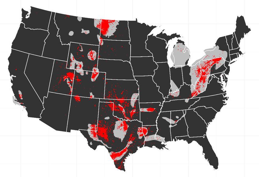
Abstract
This paper estimates the effect of the shale oil and gas boom in the United States on local economic
outcomes. The main source of exogenous variation to be explored is the location of previously
unexplored shale deposits. These have become technologically recoverable through the use of
hydraulic fracturing and horizontal drilling. I use this to estimate the localised effects from resource
extraction. Every oil- and gas sector job creates about 2.17 other jobs. Personal incomes increase by
8% in counties with at least one unconventional oil or gas well. The resource boom translates into an
overall increase in employment by between 500,000 - 600,000 jobs. A key observation is that, despite
rising labour costs, there is no Dutch disease contraction in the tradable goods sector, while the non-
tradable goods sector contracts. I reconcile this finding by providing evidence that the resource boom
may give rise to local comparative advantage, through locally lower energy cost. This allows a clean
separation of the energy price effect distinct from the local resource extraction effects.
Key words: Resource boom, fracking, shale, spillovers, natural gas, energy prices
JEL: Q33; O13; N52; R11; L71
This paper was produced as part of the Centre’s Productivity Programme. The Centre for Economic
Performance is financed by the Economic and Social Research Council.
I would like to thank Tim Besley, Jon de Quidt, Jon Colmer, Mirko Draca, Claudia Eger, Jakob
Fetzer, Christian Fons-Rosen, Maitreesh Ghatak, Benjamin Guin, Sam Marden, Hannes Mueller,
Gerard Padro-i-Miquel, Pedro Souza, Daniel Sturm, Kelly Zhang and seminar participants at LSE,
CEP, Oxford University and IAE Barcelona for helpful comments. In addition, I would like to thank
Simen Gaure for developing the lfe package for R and Tu Tran at the EIA for kindly sharing some
data.
Thiemo Fetzer is a PhD student at the London School of Economics and an Occasional
Research Assistant for Centre for Economic Performance, London School of Economics.
Published by
Centre for Economic Performance
London School of Economics and Political Science
Houghton Street
London WC2A 2AE
All rights reserved. No part of this publication may be reproduced, stored in a retrieval system or
transmitted in any form or by any means without the prior permission in writing of the publisher nor
be issued to the public or circulated in any form other than that in which it is published.
Requests for permission to reproduce any article or part of the Working Paper should be sent to the
editor at the above address.
T. Fetzer, submitted 2014.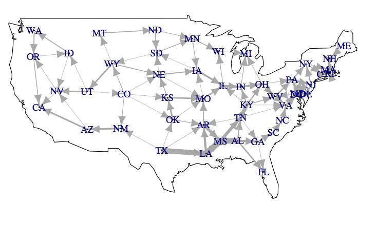
1    Introduction
The role of energy prices and its relationship with economic aggregates such as
employment, wages, and output has been a key concern for academic economist
since the oil price shocks in the 1970s (Berndt and Wood (1975)). A second literature
that developed around the same time was studying the impact of resource booms
on economic outcomes, originally at the aggregate level (Bruno and Sachs (1982),
Corden and Neary (1982a)) and then increasingly through micro-econometric stud-
ies (see Michaels (2011), Black et al. (2005)). The key empirical observation from
this literature was that resources can be, both a blessing and a curse. This paper
aims to link these two strands of literature. I exploit the recent energy boom in the
US as a window through which I can study both, the local effects of lower energy
prices and the local effects of the extraction activity itself. I show that it may be the
combination of these two forces that can help explain why a resource boom may be
a disease for some and a blessing for other countries.
    The identification will rely on two sources of arguably exogenous variation.
First, I exploit spatial variation in resource extraction of shale deposits that became
recoverable due to technological advances in drilling technology. The second source
of exogenous variation is driven by the implied changes in the energy production
geography of the US; moving natural gas production from the South to the Mid
West and the North East of the country does not have the existing pipeline capacity
to take the produce to market where the willingness to pay is highest; this generates
distinctly lower gas prices.
    In the last step, I combine the findings from these empirical approaches and
highlight that they may help us understand why there is no resource curse in sec-
tors that may be particularly vulnerable to it.
    It is important to highlight the context in which this recent energy boom is
happening. Since the early 2000s, US domestic natural gas and oil production was
in decline and the imports of crude and natural gas became even more important
as they had already been. Employment in the natural gas and oil extraction sector
was at its lowest since 1972.
    In 2012, the picture is vastly different. The transition that was achieved in the
last 7 years falls short from being a miracle. The US, in 2012, is least dependent
on foreign energy imports than it ever was since 1973. This is attributed to im-
provements in energy efficiency and the development of biofuels. However, the
most important contributing factor is the development of unconventional resource
extraction technology known as hydraulic fracturing or “fracking” that has lead to
a mining boom across the US. The hydraulic fracturing technology, together with
horizontal drilling made vast shale deposits accessible, that could previously not

                                           2
be economically exploited. As a consequence, employment in the mining sector has
reached levels not seen since the early 1990s. But do these employment gains have
significant spill-over effects into different sectors at the locations where resource
extraction is actually taking place? It is - by no means - clear, whether one should
expect significant employment gains in the non-mining sectors. The development
literature has highlighted that it strongly depends, among others, on the type of
resources (Boschini (2007), Mehlum et al. (2006)), the quality of the institutions (Vi-
cente (2010),Sala-i Martin and Subramanian (2003),Robinson et al. (2006),Monteiro
(2009), Caselli and Michaels (2012), Ross (2006)), the potential for input demand
linkages (see Aragón and Rud (2013)) and the extent to which revenues are in-
vested locally (Caselli and Michaels (2012)).
The first contribution of this paper is to quantify the extent of the local effects
due to the recent resource boom. I show that many economic aggregates, such as
local employment, payroll, labour force participation and unemployment respond
quite significantly. In the next step I highlight that this is driving up local wages
across the sectors, giving rise the the possibility of there being a resource curse. In
the third step I find no evidence that the manufacturing sector suffers from Dutch
disease style contraction, while the non-tradable goods sector does.
In the last section I explore whether locally cheaper energy may explain this
finding. Energy is a key factor of production for many production processes - both
directly and indirectly, through intermediate goods consumption. The literature
on electricity prices and provision has highlighted the relevance and importance of
cheap and in particular, reliable energy (see e.g. Rud (2012), Abeberese (2012) and
Fisher-Vanden et al. (2012)) or Dinkelman (2011), who studies the labour market
effects of electrification in South Africa. In the case of the US, Kahn and Mansur
(2013) show that electricity prices affect firm location decisions, while Severnini
(2013)’s analysis suggests that low energy prices in the historical context may have
created agglomeration clusters. I proceed to show that indeed - energy intensive
tradable goods sectors - do expand, giving initial credence to this mechanism.
Following this I show that natural gas and electricity become significantly cheaper
in counties with shale deposits from the mid 2000s onwards, suggesting that higher
labour costs may be offset with lower energy bills. I show that the effect is particu-
larly pronounced in places that face significant pipeline capacity constraints. Bind-
ing outflow capacity forces the additionally extracted natural gas to be consumed
locally, putting downward pressure on local prices.
In the last step I provide a small back of the envelope calculation that indicates
that the drop in energy prices offsets the increase in labour costs, which may explain
why the local non-tradable goods sector contracts, while the tradable goods sector
doesn’t. This highlights that a key to understanding whether Dutch disease style
3contractions do occur, depends on the nature of the resource and whether there
are significant trade costs associated with the export of the latter. This ties in well
with the arguments in Boschini (2007), who argue that the type of resource matters
for whether a country actually suffers from a resource curse. They mainly argue
that this is driven by the degree to which the resource can be appropriated. The
mechanism I explore here highlights that it depends on the extent of trade costs
and frictions, as these create locally lower energy prices.
The paper is organised as follows. I begin with a very brief conceptual frame-
work to guide the empirical analysis. In the third section I discuss the main data
sources used. The fourth section then proceeds to establish the main results, while
the fifth section focuses on the proposed mechanism of lower natural gas prices.
The last section concludes.
2 Conceptual Framework
Before discussing the data used in this paper and the empirical specifications, I
want to present a simple conceptual framework to fix some ideas and to motivate
the empirical analysis.
I build on the simple partial-equilibrium framework in Corden and Neary (1982b).
I assume that there are three sectors: the resource or energy production sector, a
tradable goods sector and a non-tradable goods sector. These are indexed with
E, T, NT and have production functions E = Ah( NE ), YNT = Bg( NNT ) and YT =
f ( NT , E). This simple formulation implicitly assumes that the tradable goods sec-
tor is relatively more energy intensive than the non-tradable goods sector. All three
sectors compete for an immobile factor labour. The price of tradable goods serves
as the numeraire. In the first exercise, I assume that energy prices and the price
of tradables is fixed and only wages and the price of non-tradables may respond
to a productivity shock in the resource extraction sector. This mimics the case of a
small open economy and gives rise to the classical results as in Corden and Neary
(1982b). In the second exercise, I model a wedge in local energy prices that is a
function of the bindingness of pipeline capacity constraints (e.g. a lack of takeaway
capacity). This generates a local market for energy and thus implies that there is a
feedback from lower energy prices. Households have simple Cobb-Douglas utility
over consumption of tradables and non-tradables.
u(YT , YNT ) = α T log(YT ) + α NT log(YNT )
Income in this economy is simply y = w + θπ E , where π E are the profits that
accrue in the energy production sector and θ is a measure indicating the extent
4to which these profits go to local owners of the mineral resources. The demand
d = α y
functions for non-tradables is simply YNT NT p NT . The market clearing condition
in the labour market requires:
d
NNT + NTd + NEd = 1
.
where the labour- and energy demand functions solve the following first order
conditions.
p E Ah0 ( NEd ) = w
p NT Bg0 ( NNT
d
)=w
Two for the tradable sector:
p T f 1 ( NTd , Ed ) = w
p T f 2 ( NTd , Ed ) = p E
For fixed energy prices, an increase in the productivity in the resource extrac-
tion sector, has three effects. Firstly, the increase in productivity is going to lead to
an overall increase in aggregate economic activity and GDP per capita. The second
and third effects are concerned about the effect on wages and the implied impact
on the allocation of labour across sectors. First, there is the resource movement effect.
As labour demand by the resource sector increases, overall wages go up. This im-
plies that the marginal cost of production for non-tradables and tradables increase.
Hence, the employment shares of these sectors contract. There is a direct factor
price induced structural transformation. Graphically this is indicated in Figure 1.
The second effect is the so-called spending effect. Higher equilibrium wages drive
up local incomes y, which is inducing an outward shift in the demand for tradables-
and non-tradables for a given level of prices. This increased demand leads to an
increase in production in the non-tradables sector, thus, partly offsetting the im-
plied contraction due to the resource movement effect. Wages increase even further
and thus, lead to a further contraction of the tradable good sector. The sum of
the spending and resource movement effect suggests an unambiguous increase in
wages and thus, a contraction in the tradable goods sector, but not necessarily in
the non-tradable goods sector due to the spending effect. The degree to which the
spending effect may offset the resource movement effect depends on the elasticity
of demand for non-tradables with respect to income.
Consider now the case of variable energy prices. In particular, I assume that en-
5Figure 1: Resource Movement Effect
Figure 2: Resource Movement and Spending Effect
6ergy prices p̄ E are exogenously given, but local energy prices p E may be lower than
p̄ E . Local energy price differentials reflect the extent to which energy is tradable.
For energy, such as natural gas or electricity there are mechanic trade costs, as the
transport of the commodity uses up part of the commodity itself.1 I assume that
local energy prices are given as:
p E = τ ( E) p̄ E
with τ ( E) < 1. The degree of the price wedge depends on a set of characteris-
tics, such as pipeline transmission constraints and the physically implied transport
costs.
Given this reduced form representation of the local energy market, there is now
a distinct margin through which an increase in productivity in energy production
affects the tradable goods sector. With endogenous local energy prices, the increase
in the productivity of the energy production sector is correlated with lower local
energy prices, which may provide insurance against the increase in labour costs.
A reduction in the energy prices does not have a direct effect on the non-tradable
goods sector, but it does have an impact on the energy and the tradable goods
sector. First, it is going to moderate the initial movement of labour into the energy
sector as the marginal returns are now decreasing in the level of output and second,
the lower energy price is going to increase the demand for labour by the tradable
sector depending on the degree of complementarity. This further increases wages,
while hurting the non-tradable goods sector, as the latter is not able to benefit from
lower energy prices; the key observation is that an energy price effect may now
generate ambiguous effects for all three sectors.
The degree of ambiguity depends on the relative strength of the resource-movement
effect compared to the spending effect and the energy price effect. The key vari-
ables of interest here are the labour intensity relative to the labour intensity for the
interplay of the energy price effect and the spending effect and the income elastic-
ity of demand for non-tradables, which measures the degree to which the spending
effect affects the non-tradable goods sector.
The ambiguous predictions for the relative employment shares make this very
much an empirical question. I will proceed in three steps that follow naturally from
this analysis.
1 For natural gas, 11% of the extracted natural gas is used in the transmission process by compressor
stations along the natural gas pipeline grid. For electricity, aggregate transmission losses account for 7%
of gross electricity generation.
73 Data
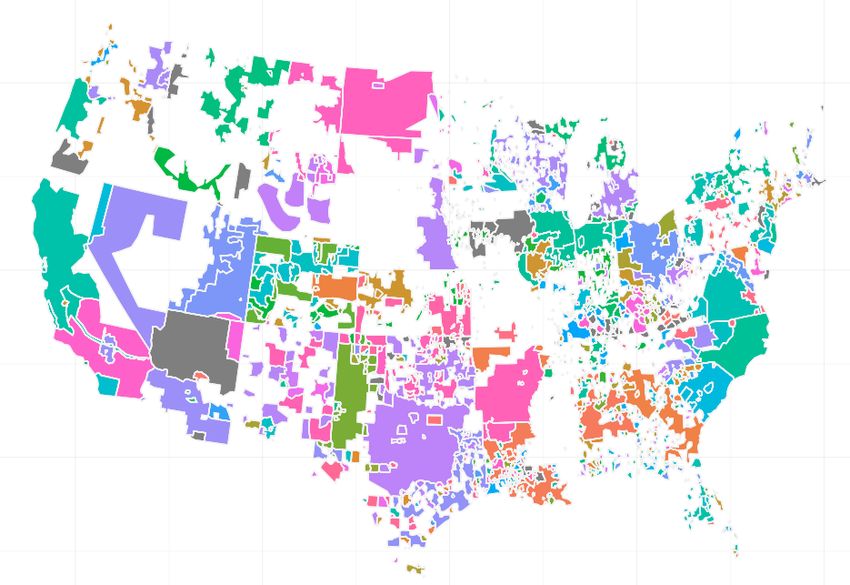
Shale Plays, Oil- and Gas Well Location Data
The key empirical design will be simple intention-to-treat exercises exploiting geo-
graphic variation in the availability of unconventional oil and gas resources. This
data was obtained from the Energy Information Administration and the US Geo-
logical Survey and is presented as the grey areas in Figure 3.
The second main source of data is a set of geocoded locations of actual uncon-
ventional oil or gas wells where unconventional techniques involving horizontal
drilling and hydraulic fracturing are applied. This data was derived from various
state-level sources and the data disclosure website Frac Focus. The data is discussed
in further detail in Appendix A.1. Based on these data I construct a cross-sectional
dummy indicating the presence of an unconventional well in a county by 2012. This
dummy variable provides cleaner treatment assignment and does not merely reflect
the intention to treat, since not all shale resources are currently being actively pur-
sued. The resulting map of well locations is presented in Figure 3. The reason for
using the cross-section of well locations is one of data constraints; not for all wells
in the sample do I have data on the actual timing of when a well was constructed.
The unconventional shale gas and oil boom commenced in 2005, however, the tim-
ing varies across shale plays. I have the exact dates of when drilling operations
commenced for a set of states, appendix A.1 shows that new well construction is
significantly occurring from the mid 2000s onwards, which coincides well with the
anecdotal accounts.
Sectoral Employment
They key outcome variables studied in this paper is annual sectoral employment, as
obtained from the the Longitudinal Employer-Household Dynamics dataset main-
tained by the US Census Bureau (see Davis et al. (2006) for a discussion). This
dataset produces Quarterly Workforce Indicators (QWI) that provide details up to
4-digit NAICS industry codes. The data covers 96% of all employment in the US
and is developed to provide researchers with a very fine spatial- and temporal res-
olution that can be further disaggregated by firm- characteristics, such as firm size
and age or by individual employee characteristics such as age, educational attain-
ment and race. The second key variable of interest is the earnings per worker data,
which provides the average monthly earnings for a worker in a sector and county
in a given quarter, provided that this worker has been with the firm for the duration
of the whole quarter. This variable will be used as a proxy for wages. Since estimat-
ing high dimensional fixed effects can be computationally very heavy, I reduce the
8Figure 3: Location of Unconventional Wells in 2012 (red dots) and Shale Plays (grey)
time-dimension by a factor of four by constructing sector specific annual average
employment figures. This induces a loss of signal, however, it makes it feasible to
run the regressions on a simple desktop computer.
Due to non-disclosure constraints there are some issues as the data is infused
with noise. These are discussed in detail in A.4 and all results are robust when
accounting for these non-disclosure constraints. A second caveat is that the data are
not available for all states from 1998 onwards. As a robustness check, I construct a
balanced panel filling the missing observations with the county-business patterns
database that has been extensively used in the past (see e.g. Kahn and Mansur
(2013), Mian and Sufi (2011), or Rosenthal and Strange (2001)).
Energy Price Data
I construct county-level annual electricity and natural gas prices using two sources.
For the electricity prices I use the Annual Electric Power Industry Report by the
Energy Information Administration, which provides for each of the roughly 3,000
electric utility companies the revenues and the quantity of electricity sold to com-
mercial, residential and industrial customers. This is used to construct an average
price per supplier. The majority of the utility companies serve individual munic-
ipalities or relatively small spatial areas. Using data on the location of electricity
delivery equipment, I construct the service area of each municipality and the com-
9pute the average price charged.
I proceed similarly for the natural gas prices using data collected by the En-
ergy Information Administration under Form EIA-176. This provides revenues and
quantities of gas sold in a state and year for a local distribution company. The
service areas were constructed based on confidential data from the EIA; it is only
available for the year 2008, implying that changes in the service areas are not re-
flected in my data. The average price of gas in a county is proxied by the simple
averages of the prices charged by local distribution companies that service cus-
tomers in a county. More details on the construction of these data are detailed in
appendix A.3.
Pipeline Capacity Constraints
The Energy Information Administration provides data on state-to-state physical
pipeline capacity at an annual level as well as annual state-to-state pipeline flows.
Figure A4 plots the resulting net physical capacity flows. For each state the annual
data provides information how much natural gas is flowing to all its neighbouring
states. Based on this, I can compute a state level measure of the bindingness of the
existing physical outflow- and inflow capacity. Let P be the set of states that are
neighbouring state s, and C ps be the direct physical pipeline capacity connecting
state p ∈ P with state s, while Fps is the actually observed flow.
I simply compute
∑ p∈P Fps
Os =
∑ p∈P C ps
as a measure of the bindingness of outflow capacity. Similarly, I compute Is
as a measure of the bindingness of inflow capacity. It is well-established that a
key ingredient driving local natural gas prices is the bindingness of pipeline ca-
pacity constraints; for electricity markets, this is very similar and has recently been
analysed by Ryan (2013) in the Indian context.2
I construct the measure using the average capacity for the period 2000-2005 and
the average flows for that period. Averaging helps remove year-on-year variation
e.g. induced by weather phenomena or other shocks, such as hurricanes, which may
adversely affect production in the outer continental shelf in the Gulf of Mexico.
The key intuition behind the various measures is that relatively binding outflow
capacity leads to locally lower natural gas prices, as additional local production
needs to be locally consumed. This variation will be exploited to identify the effect
2 On the natural gas spot market, the role of transmission constraints were very visible in recent
months due to the strong winter driving up energy demand. Natural gas prices on the Algonquin
Citygate, near Boston, peaked at $ 95.00, averaging at $ 11 per cubic foot; prices in Louisiana peaked
only at $ 9.00 and averaged at $ 4.55 per cubic foot.
10of the shale boom on local energy prices.
I now proceed to present the main estimating equation along with the key re-
sults in turn.
4 Empirical Strategy and Results
This section presents the main estimation strategy along with the key results. I
use two main specifications throughout the paper. The first one is to illustrate the
overall effect of the recent shale-gas and oil boom. For this, I consider the left-hand
side variables in levels as the conceptual framework indicates an overall economic
expansion due to the technological progress in the resource extraction sector. For
these exercises I use a simple instrumental variables exercise using the presence
of shale-resources (the intention to treat) as an instrument for the cross section of
unconventional wells that were present by the end of 2012.
ycist = αci + bst + ∑ γi × Shalec + X 0 β + νcist (1)
i
where αci is a set of county industry fixed effects, bst is a set of state-time fixed
effects, X is a set of other controls3 and Shalec measures the share of the land area
in a county that is covered by unconventional shale resources. Standard errors will
be clustered at the state-level unless otherwise stated.
The main instrumental variables specification is
ycist = αci + bst + ∑ ηt × Yeart × Anywellc + X 0 β + ecist (2)
t
where Anywellc is a dummy variable that is equal to 1 in case there is an uncon-
ventional well located in a county by 2012. These are instrumented with the set of
interactions Yeart × Shalec . These specifications will allow the visual presentation of
most regression results, however, I also report less demanding specifications where
I split the data into a pre- and post period with 2008 being the cutoff year.
The second set of exercises aims to highlight the impact of the expansion of
the mining sector and how this affects the labour allocation across sectors. For
this exercise, I instrument the share of mining sector employment with a post 2008
variable interacted with the share of a county’s surface that has shale resources.
That is the specification becomes:
3I construct a set of heating- and cooling degree days controls using the daily minimum- and maxi-
mum temperature data based on the PRISM dataset, which comes at a spatial resolution of roughly 4 x
4 kilometres. See appendix A.6 for more details.
11\
ycist = αci + bst + η MiningSectorShare + X 0 β + ecist (3)
where the first stage is
MiningSectorSharecst = αc + bst + γ × Post2008 × Shalec + X 0 β + νcist (4)
As the prediction of the conceptual framework for the labour market was about
the relative sector sizes, this design mimics the conceptual framework closely.
The empirical analysis will proceed in three steps. First, I show that there is
indeed a significant expansion of oil- and gas employment in areas with shale re-
sources, and an overall economic expansion in other economic aggregates such as
local area income, and employment. Most of the effect is driven by increased labour
force participation and less unemployment, while I do not observe significant gains
in population. I will use the boom in the mining sector to measure the extent of
spill-overs. This is a margin that is not incorporated by the simple model, which,
however, moderates any Dutch disease style contraction in the non- mining sec-
tors. I then show that the mining sector expansion is correlated with significantly
higher monthly earnings across most sectors; this is the only unambiguous predic-
tion from the conceptual framework, however, there is some heterogeneity due to
the different skill requirements across sectors. In the third step, I present results
on the employment shares, which highlights that the simple logic of the resource-
movement and spending effect do not provide the expected results. I then try to
reconcile these findings by providing evidence of distinctly lower energy prices
facing the tradable goods sector. A small back-of-the envelope calculation suggests
that indeed - lower energy costs may explain why there is no contraction in the
tradable goods sector relative to the non-tradable goods sectors.
Step 1: Shale Resources and Economic Expansion
I first present evidence on the impact of shale resources on overall economic expan-
sion. I document this in three individual steps. First, I show that there is a dramatic
expansion in oil- and gas sector that sets on from about 2005 onwards.
In the next step, I study overall local labour market outcomes. I document dra-
matic increases in overall employment, labour force participation and a significant
reduction in unemployment rate. I show that this expansion extends beyond the
mining sector, indicating that there are significant spill-overs. I use this to estimate
a job-creation elasticity, indicating the number of jobs that are created for each oil-
and gas sector job.
The third part documents the impact on local area income and payroll; this
121.5
1.0
Estimated Effect
0.5
0.0
2001 2004 2007 2010
Year
Employment (IV) Employment (Reduced Form) P-Value 0.10 0.05 0.01
Figure 4: Expansion of Oil- and Gas Extraction Sector Employment
highlights that there is an overall increase in economic activity.
The results from estimating models 1 and 2 are best presented graphically by
plotting the estimated coefficients η̂t and γ̂t , all accompanying tables can be found
in the online appendix.
Oil and Gas Sector Expansion Figure 4 presents the results from estimating
models 1 and 2, where I use the log of employment in the mining sector as the
dependent variable. The pattern is very similar when using the share of oil- and
gas sector employment as the dependent variable.
The coefficient plots are slightly unconventional. The line presents the estimated
coefficients in the different years for the IV specification in red and the intention-
to-tread reduced form in blue. The shade around the line becomes less opaque as
the estimated coefficients approach p-values near conventional significance levels.
This highlights that the estimated effects are insignificant before 2006, which coin-
cides well with the general accounts that fracking has only become a widespread
technology used from the mid 2000s onwards.
The estimated effects indicate how dramatic the expansion has been. The IV
coefficient suggests that places with unconventional oil or gas extraction activity
13have experienced a growth in mining sector employment by 1.38 log points in 2012
relative to control counties.4 The intention-to-treat estimates are, as expected, sig-
nificantly lower suggesting an increase by 0.4 log points or 49% in 2012. Table 1
presents the results from pooling into a pre- and post 2008 period. This year was
chosen as the dynamics in most of these controls appear to be picking up from
this point onwards. The results do not change significantly, if I use a different
break year. Clearly, there are some concerns about the onset of the financial crisis
with Lehman brothers collapse in late 2008. This will be addressed in detail in
various robustness checks. Column (1) presents the results for the mining sector,
giving very similar results, suggesting an increase in mining sector employment by
around 1 log points.
Overall Local Economic Activity In the simple conceptual framework, the
only source for change in overall levels of local income is due to the technologi-
cal progress in the oil- and gas sector. Hence, the increase in employment in the
oil- and gas sector is not sufficient to highlight that there is indeed a local economic
expansion that can be ascribed to the boom in the oil and gas sector.
I now document that many economic aggregates respond to the boom in the
mining sector, indicating that there is indeed an increase in overall economic ac-
tivity. The key variables I consider are measures of labour market activity, such
as unemployment, overall employment, non-mining sector employment, local area
income and local area overall payroll.5
Figure 5 presents the core results for a set of economic indicators. The top panel
presents the IV results, while the bottom panel draws the estimated coefficients for
the intention to treat exercises. The opacity of the line is proportional to the p-value
of the estimated regression coefficient. The pattern that emerges is consistent.
Columns (2)-(7) of table 1 presents a regression version of the graphs. The re-
sults indicate a significant expansion in non-mining sector expansion (see column
3). This expansion is coming from increased labour force participation and signifi-
cantly lower unemployment, as is indicated in columns (4) and (5). The coefficient
suggests that overall unemployment on counties with unconventional oil and gas
is about 1.1 percentage points lower than for control counties.
Columns (6) and (7) explore the effects on local incomes. Personal incomes
4 Note that the big increases can not simply be converted to proportional increases due to Jensen’s
inequality, see Kennedy (1981). Thats why I leave them as log-points. For small values, the linear
approximation is reported.
5 The local unemployment data is drawn from the Bureau of Labor Statistics Local Area Unemploy-
ment Rate database, while the local area income data comes from the Bureau of Economic Analysis
Regional Economic Accounts. The remaining data is from the Quarterly Workforce Indicators described
in the data section.
14Employment Income Broader Labour Market
0.20
0.15
0.3
0.15
0.10
Estimated Effect
Estimated Effect
Estimated Effect
0.2
0.10
0.05
0.1
0.05
0.00
0.0
2001 2004 2007 2010 2001 2004 2007 2010 2001 2004 2007 2010
Year Year Year
Non Mining Overall P-Value 0.10 0.05 Payroll Personal Income P-Value 0.10 0.05 0.01 P-Value 0.10 0.05 Labour Force Unemployment
Employment Income Broader Labour Market
0.06
0.04
0.09
0.03
Estimated Effect
Estimated Effect
Estimated Effect
0.04
0.06
0.02
0.03 0.01
0.02
0.00
0.00
2001 2004 2007 2010 2001 2004 2007 2010 2001 2004 2007 2010
Year Year Year
Non Mining Overall P-Value 0.10 0.05 Payroll Personal Income P-Value 0.10 0.05 0.01 P-Value 0.10 0.05 Labour Force Unemployment
Figure 5: Overall Effects on Employment, Non-Mining Employment and Local Income
Variables
increase by around 8%, while the payroll increases by roughly 20%. This already
indicates that wage levels must be rising, as the overall employment increase in
column (2) is just 10%, suggesting that wages must have gone up at least to some
extent to bridge the difference.6
I now turn to exploring the extent to which the expansion in the oil and gas sec-
tor creates spill-over job growth and the extent thereof. This is a particular mech-
anism not incorporated in the simple conceptual framework, which may moderate
any Dutch disease style contraction for local non-tradable goods producers.
Spill-Overs and Local Job Creation The expansion in the mining sector can be
used as an instrument to estimate local multipliers for job creation, as e.g. explored
in Moretti (2010). This is important in this context as positive spill-overs indicate
that local non-tradable goods sectors, who benefit from such spill-overs due to
demand linkages, may not actually contract in response of an expansion of the oil
and gas sector, as they are benefiting directly through increased demand on top
of the spending effect. In order to evaluate this, I use as instrument for oil and
gas sector employment an interaction term Post2008 × Shalec . This gives rise to the
estimates in column (2) of table 2.
6 An alternative explanation is increased working hours driving up overall payroll; this is a mechanism
that is, unfortunately, unobservable.
15In the third column I use the estimated elasticity from column (2) and multiply
this by the means of the respective employment variables.7
I study four sectors separately. The first is the overall-non mining sector em-
ployment. This suggests that for every oil and gas sector job, on average, 2.17
non-mining sector jobs are created. The effect is mainly driven by growth in
construction- and transportation sectors, which are strongly linked with the oil and
gas industry. The other main employment categories do not experience statistically
significant spill-overs. Given that overall employment in the oil and gas sector has
more than doubled between 2004 and 2013, increasing by 264,900 from 316,700 to
581,500 this translates into an increase in overall employment by around 574,833
due to the shale oil and gas boom. This represents a significant share of roughly
0.4% of all employment in the US in 2012.
Step 2: Response of Wages and Earnings
The preceding results already indicate that there must be an increase of local wages
in response to the resource boom, since the overall payroll increases more than the
overall employment as indicated in 5. I now document the effect on real wages,
highlighting that the estimated effect is a real wage increase, rather than a nominal
one, as predicted by the simple framework. 8
I estimate specification 3, predicting the share of mining sector employment
with the interaction term Post2008 × Shalec as before.
The results are presented in table 3. Column (1) suggests that an increase in
the mining sector share by one percentage point increases monthly earnings in that
sector by 6 percentage points. Columns (2) - (6) provide the respective effects for
the different sectors. Column (3) and (4) present the results for the construction and
transportation sector wages. These are directly linked to the mining sector through
mining sector demand.9 The local manufacturing and service sector wages respond
in similar fashion: a 1 percentage point increase in the mining employment share
7I only include observations up to the 95% percentile of the total non-mining sector employment. This
becomes necessary as the employment and population data is highly skewed, distorting the means when
including the upper quantiles. In the regressions, the skewness is taken care of by using logarithmic
transformation, making conditional mean regressions appropriate.
8 I construct local price-indices by combining a series of Consumer Price Indices for metropolitan sta-
tistical areas, Census regions and Census region by city size drawn from the Bureau of Labour Statistics.
I assign the CPI level to a county provided it falls in one of the metropolitan statistical areas that have
its own dedicated CPI series. For the remaining ones, I compute the weighted average of the CPI using
the Census region and city size CPI series using as weights the population of a county that falls in each
town-size class for which a separate CPI value for that respective region is available.
9 The New York Department of Energy Conservation estimates that the construction of each well
requires between 895 to 1350 truck loads, see http://www.dec.ny.gov/energy/58440.html, accessed on
15.08.2013.
16increases their respective wages by about 1.8 and 1.9 percentage points respectively.
Since the mining sector share increased by around 3 percentage points on av-
erage, suggests that real wage costs for manufacturing firms increased by roughly
5 percentage points. These results suggest that there is some heterogeneity in the
extent of the wage increase. The effect is weaker for sectors with less of a factor
demand linkage. However, overall, wages do increase significantly, which mirrors
the findings of Allcott and Keniston (2013), who study the effects of oil and gas
booms on the manufacturing sector over the last thirty years. In the appendix, Ta-
ble A4 presents the reduced form results by education group, confirming that the
strongest dynamics are observed for relatively low educational attainment levels.
The observed increase in real wages sets up the possibility for there to be a
Dutch disease style contraction in the tradable and non-tradable local sectors. In
the next step I provide results that highlight that reallocation of labour across sec-
tors in the manner suggested by the simple conceptual framework does not occur.
The manufacturing sector does neither contract nor expand, while the non-tradable
service goods sector contracts.
Step 3: Employment Shares and Labour Reallocation
The conceptual framework without endogenous local energy prices, suggest that
there be an unambiguously negative effect on the tradable goods sector, while the
response of the relative size of the non-tradable goods sector is ambiguous. The
latter depends on the strength of the spending effect.
I now explore the evolution of the sectoral shares over time. The results are
presented in table 4. The first column presents the result from specifications 2. This
gives a sense of the overall impact of well-construction on shale deposits on the
share of mining sector employment; overall, mining sector employment increased
by around 3 percentage points, more than doubling the initial mining sector em-
ployment share of roughly 2%. Columns (2)-(6) use the share of mining sector
employment as a right hand side, instrumented for by the interaction Post 2008 x
Shale as in specification 3.
Column (2) indicates that the manufacturing sector appears not to be contract-
ing. The coefficient on the share of manufacturing employment is negative but far
form being statistically significant. Column (3) suggests that a one percentage point
increase in mining sector employment increases the construction employment share
by 0.453 percentage points. The stark observation is that for locally consumed ser-
vices (column (5) and (6)), the coefficient is unambiguously negative. This suggests
that the reallocation of labour across sectors happens at the expense of the local
non-tradable goods sector, rather than at the expense of the tradable goods sector.
17This is quite at odds with the conceptual framework, which suggested that the local
non-tradable goods sector might even expand if the spending effect is sufficiently
strong. The results presented here suggest that this is not the case, i.e. the spending
effect appears to be quite week.
The next section highlights that the local tradable goods sector may even ex-
pand, despite rising labour cost. I argue that this is driven by the fact that local
energy prices drop dramatically in response of the oil and gas boom. As tradable
goods sectors are more energy intensive, this offsets the increase in labour costs.
This ties in well with the arguments in Boschini (2007), which argue that the type
of resource matters for whether a country actually suffers from a resource curse.
They mainly argue that this is driven by the degree to which the resource can be ap-
propriated. The mechanism I explore here highlights that it depends on the extent
of trade costs and frictions.
5 Local Energy Prices and Sectoral Change
In this section I focus on one key mechanism that may explain why tradable goods
sectors do not appear to contract, while other non-tradable goods sector appear to
suffer from a Dutch disease style contraction. I first present evidence that supports
this mechanism: local sectors that are energy intensive do not contract. This holds
up when controlling for the extent to which the sectors are linked to the resource
extraction sector producing inputs for the latter, and a wide array of other control
variables at the three digit industry level.
I then document that local energy prices do indeed contract significantly. Places
with unconventional oil- and gas extraction experience drops in the costs of nat-
ural gas by almost 30%. Similarly, local electricity prices go down significantly. I
document that these effects are particularly pronounced in locations that are export
constraint by the existing natural gas pipeline network, suggesting that trade costs
can indeed be made responsible for these lower factor prices.
This suggests that in the short run, the boom in the resource extraction sector
may not necessarily crowd out local tradable goods producers. It may even attract
further producers of energy intensive goods. There are anecdotal accounts suggest-
ing that this is happening in the heart of America, with fertiliser producers building
up capacity in the West of the US, taking advantage of lower energy prices there.10
In order to compare the degree to which different sectors vary in their use of
energy as a source of input, I refer to the 2002 input-output tables developed by the
Bureau of Economic Analysis. Based on these, I construct measures of natural-gas
10 Seee.g. http://www.agweek.com/event/article/id/21548/publisher_ID/80/ for recent fertiliser
plant construction in North Dakota.
18intensity and overall utility intensity at the three digit industry sector level, as there
is significant variation within two digit industry.11
Using the same data-source, I also compute the labour cost shares as well as the
degree to which each sector is linked to the mining sectors by providing inputs for
the latter. This is an important control variable as it has been identified earlier that
there are significant spillovers in the non-mining transportation- and construction
sectors, which may moderate any labour cost induced contraction. In the appendix,
Table A1 provides these respective cost shares at the two-digit industry level.
All intensity measures are at the three digit level. Unfortunately, the input-
output tables do not have the same sectoral break-up as the employment data. In
particular, the retail- and wholesale trade sectors are all pooled together at the two
digit industry level. Thats why I focus the main results on just the manufacturing
sector as there I have significant variation in energy intensity. I then successively
add more sectors in the control group to highlight that the estimated coefficient
and patterns stay virtually the same and the results become even stronger.
Energy Intensity and Sector Specific Expansion In order to capture the sec-
tor specific variation in energy intensity, I modify the estimating equation 1 by
adding interaction terms with the sector specific energy intensity. The estimating
equation then becomes:
ycist = αci + bst + κ × Post2008 × Shalec × EnergyIntensityi
+ γ × Post2008 × EnergyIntensityi + X 0 β + νcist
where as left-hand side I use the log of sector specific employment. In order to
capture heterogeneity by different factor input intensities, I add further interactions.
The results can be found in table 5.12
The first four columns constrain the analysis to only include the tradable goods
11 In order to measure this, I compute the cost shares of natural gas in the input costs. For natural gas,
I sum up all the purchased values from companies working in the Natural Gas Distribution, Oil- and
Gas Extraction 21100 and the Natural Gas Pipeline Transportation sectors (NAICS Codes 221200, 21100,
486000 respectively). This gets as close as possible to the input cost shares of natural gas. For the broader
utility cost shares, I include all the above sectors and all electric utilities, that is private Electric Power
Generation, Transmission and Distribution and State and local government electric utilities (NAICS
Codes 2211000 and S00101, S00202).
I construct both measures of direct utility consumption as well as indirect utility consumption, indi-
rectly used through the consumption of intermediary inputs.
12 Note that the standard errors are clustered at the Workforce Investment Board Area level (WIA).
This are regional entities created to implement the Workforce Investment Act of 1998. There are about
7-8 counties per workforce investment board area, rendering them spatially still significant in size to
account for spatial correlation. An appealing feature of the WIA is that they are designed to include
counties with similar economic structure, to ensure that the services under the Workforce Investment
Act can be direct to the local needs.
19industries.13 While the coefficient on the simple interaction of the time dummy
with the shale deposit indicator is negative but insignificant, the coefficient on the
energy intensity interaction is positive and statistically significantly different from
zero. This coefficient does not change when adding more interactions as control
variables, such as the downstream linkages or the labour cost share. Columns (5) -
(7) include subsequently more sectors. In column (5) I add the non-tradable goods
sector as control. As expected, the results get stronger.
This suggests that energy intensive tradable goods sector are actually benefiting
from being on the shale. In the next section I highlight that this may be due to sig-
nificantly lower energy prices, which allows tradable goods producers to compete
despite rising labour costs.
Trade Costs and Local Energy Prices I show that local energy prices actually
go down significantly. This reduction in energy prices is particularly observed for
states with shale deposits but that have relatively little slack natural gas pipeline
outflow capacity.
I estimate specifications 1 and 2 as before, however, now using local utility and
electricity prices as left-hand side variables.
Figure 6 displays the estimated coefficients for local natural gas prices. It ap-
pears that well before 2008 - if anything - natural gas prices in counties with shale
deposits had actually been higher than in the rest of the US. From 2008 onwards,
this picture changes. By 2012, natural gas on places with shale deposits and active
resource extraction, was - on average - almost 30 percent cheaper than in the rest of
the US.
Table 5 presents the reduced form results when exploring this relationship in a
more systematic manner. In column (1) I present the reduced form effect of being
on the shale on natural gas prices by all uses. This suggests that counties with shale
deposits had - on average - 2.2% lower natural gas price. Column (2) refines this
to focus on industrial use gas prices, which are particularly relevant for tradable
goods producers. This highlights that the overall effect is driven by the price for
industrial users. This makes sense as the latter is a lot more flexible as prices to
residential consumers are typically regulated and quite sticky.
In column (3) and (4) I explore that it is actually a lack of physical pipeline
capacity (and thus trade costs), that drive a significant portion of the observed
natural gas price drop. States with relatively binding outflow capacity observe
stronger price drops. This is intuitive. An increase in local production has to
13 The classification is based on the four digit sector classification used in Mian and Sufi (2011). I
exclude the mining sector and the 3-digit sector 324, Petroleum and Coal Products Manufacturing, as
this sector captures the 144 oil refineries that are extremely concentrated in a few counties; furthermore,it
represent a significant outlier as more than 70% of their input costs are direct costs for oil.
200.6
0.3
Estimated Effect
0.0
-0.3
2000 2004 2008 2012
Year
Figure 6: Natural Gas Prices for Industrial Consumers for Counties on Shale Deposits
with a well by 2012
reduce local prices if the additional production can not be exported. In column (5)
I use the relative bindingness of outflow-capacity to inflow-capacity. This measures
the overall degree to which a state has slack capacity available, where that slack
capacity could be indicating that local production is displacing imports or can not
be exported due to outflow constraints.
Columns (5)-(7) present the results for average electricity prices. The results are
similar, but statistically a lot weaker. This is obvious as one way to avoid pipeline
capacity constraints is through the conversion of natural gas into electricity, where
transmission constraints may be less binding. Hence, this suggests that the results
may be driven mostly by lower natural gas prices.14
I now present a small back of the envelope calculation to see whether the ob-
served energy price drops may indeed offset the labour cost increases.
Mining Sector Expansion and Local Energy Prices In the third step, I esti-
mated the effect of the relative expansion of the mining sector on sectoral wages.
This suggested that manufacturing wages increased by 1.6 percentage points for
every 1 percentage point increase in the share of mining sector employment.
In Table 7 I present the results from the same analysis, however, replacing the
14 This is confirmed when performing the same analysis for the overall energy intensity presented in
table 5, but now focusing only on the directly consumed natural gas. The results are presented in the
appendix in table A5.
21electricity and gas prices on on the left hand side. The results are quite strong:
column (1) studies overall natural gas prices. An increase in mining sector share
by 1 percentage points reduces natural gas prices by 2.4 percentage points. This
effect is even stronger for industrial use natural gas prices, where the elasticity is
6, evidenced in column (2). Column (3) looks at electricity prices, again I see a
significant negative effect.
Can the drop in energy prices offset the increased labour costs and thus, mod-
erate a Dutch disease style contraction in energy intensive sectors as is suggested
by the results presented in the previous section? Given that the overall energy in-
tensity is 5.3 percent for the manufacturing sector, while the labour cost share is
19.2%, this implies that the energy costs must go down by 3.6 times the amount
that labour costs have gone up in order to compensate the labour cost increases.15
The results presented here are well in this ball-park. The increase in labour
costs was estimated to be around 1.6 percent, while industrial gas prices have gone
down by around 6 percent for a one percentage point increase in mining sector
6
employment. Hence, the factor is actually 1.6 = 3.75, suggesting that total operating
costs may actually have stayed the same - i.e. there is full compensation in form of
lower energy costs offsetting the labour costs.
This does not affect the non-tradable goods sectors, who may benefit from lower
energy prices but too a lesser extent as their average energy cost shares are signifi-
cantly lower.
6 Conclusion
The existing literature has highlighted that resource booms tend to benefit the lo-
cal service sector (see Kuralbayeva and Stefanski (2013); Michaels (2011); Sachs and
Warner (1999). Depending on the institutional environment, there is some sugges-
tive evidence that resource booms create fiscal surpluses which may induce growth
in public sector employment (see e.g. Robinson et al. (2006), Baland and Francois
(2000)). Lastly, resource booms, depending on the degree of local demand linkages
should lead to a boost in sectors that provide inputs for the mining industry (see
e.g. Marchand (2012) and Black et al. (2005)). On the other hand, the literature on
Dutch disease has highlighted that there may be adverse effects on local tradable
goods producers, as they can not pass on higher labour costs on to final goods
consumers.
In this paper I provide evidence that sectoral reallocation appears not to hap-
pen as described in the classic Dutch disease literature. I do not explore whether
15 Referto table A1 for the average utility cost shares at the two digit sector level derived from the
input-output tables.
22agglomeration externalities may explain why this does not happen (as e.g. Allcott
and Keniston (2013)), but focus on a different and much more simple mechanism.
First, my results suggest that the spending effect, which positively affects the non-
tradable goods sector share is quite weak. In addition to the resource movement
effect, my results indicate that local energy prices may explain why there is no con-
traction in the tradable goods sector, while there is for the non-tradables sector. The
argument is simple. The resource boom creates a local comparative advantage in
form of lower energy prices. It is questionable whether this is an effect that persists.
This depends on the nature of the transport cost induced energy price differentials.
If the price differentials are purely due to a lack of transmission capacity, arbitrage
conditions will imply that these missing transmission links will be build to arbi-
trage the price differences away. On the other hand, a significant share of energy
costs are due to transmission losses, which would make locally lower energy prices
a persistent feature. Further research is needed to highlight whether this is the case.
References
Abeberese, A. B. (2012). Electricity Cost and Firm Performance: Evidence from
India. mimeo.
Abowd, J. (2005). Confidentiality Protection in the Census Bureaus Quarterly Work-
force Indicators. US Census Bureau.
Abowd, J. and R. Gittings (2012). Dynamically consistent noise infusion and par-
tially synthetic data as confidentiality protection measures for related time-series.
US Census Bureau . . . (2009).
Allcott, H. and D. Keniston (2013). Dutch Disease or Agglomeration ? The Local
Economic E ects of Natural Resource Booms in Modern America.
Aragón, F. and J. Rud (2013). Natural resources and local communities: evidence
from a Peruvian gold mine. American Economic Journal: Economic . . . , 1–31.
Baland, J. and P. Francois (2000, April). Rent-seeking and resource booms. Journal
of Development Economics 61(2), 527–542.
Berndt, E. and D. Wood (1975). Technology, prices, and the derived demand for
energy. The Review of Economics and Statistics 57(3).
Black, D., T. McKinnish, and S. Sanders (2005). The Economic Impact of the Coal
Boom and Bust. The Economic Journal (March 2004).
23Boschini, A. (2007). Resource curse or not : A question of appropriability. The
Scandinavian Journal . . . 109(3), 593–617.
Bruno, M. and J. Sachs (1982). Energy and Resource Allocation: A Dynamic Model
of the Dutch Disease. The Review of Economic Studies.
Caselli, F. and G. Michaels (2012). Do Oil Windfalls Improve Living Standards?
Evidence from Brazil. mimeo (May), 1–43.
Corden, W. and J. Neary (1982a). Booming Sector and De-Industrialisation in a
Small Open Economy,. The Economic Journal 92, 825–848.
Corden, W. and J. Neary (1982b). Booming Sector and De-Industrialisation in a
Small Open Economy. The Economic Journal 92(368), 825–848.
Daly, C., M. Halbleib, and J. Smith (2008). Physiographically sensitive mapping
of climatological temperature and precipitation across the conterminous United
States. International Journal of Climatology 28(15).
Davis, S. J., R. J. Faberman, and J. Haltiwanger (2006, June). The Flow Approach
to Labor Markets: New Data Sources and MicroMacro Links. Journal of Economic
Perspectives 20(3), 3–26.
Day, A. and T. Karayiannis (1999). Identification of the uncertainties in degree-day-
based energy estimates.
Dinkelman, T. (2011). The Effects of Rural Electrification on Employment : New
Evidence from South Africa. The American Economic Review 101(December), 3078–
3108.
Fisher-Vanden, K., E. T. Mansur, and Q. J. Wang (2012). Costly Blackouts? Mea-
suring Productivity and Environmental Effects of Electricity Shortages. NBER
Working Paper 17741.
Kahn, M. E. and E. T. Mansur (2013, May). Do local energy prices and regulation af-
fect the geographic concentration of employment? Journal of Public Economics 101,
105–114.
Kennedy, P. (1981). Estimation with Correctly Interpreted Dummy Variables in
Semilogarithmic Equations. American Economic Review.
Kuralbayeva, K. and R. Stefanski (2013). Windfalls, Structural Transformation and
Specialization. Journal of International Economics, 1–63.
24You can also read