Lessons from a high-CO2 world: an ocean view from 3 million years ago - Recent
←
→
Page content transcription
If your browser does not render page correctly, please read the page content below
Clim. Past, 16, 1599–1615, 2020
https://doi.org/10.5194/cp-16-1599-2020
© Author(s) 2020. This work is distributed under
the Creative Commons Attribution 4.0 License.

Lessons from a high-CO2 world: an ocean view
from ∼ 3 million years ago
Erin L. McClymont1 , Heather L. Ford2 , Sze Ling Ho3 , Julia C. Tindall4 , Alan M. Haywood4 ,
Montserrat Alonso-Garcia5,6 , Ian Bailey7 , Melissa A. Berke8 , Kate Littler7 , Molly O. Patterson9 , Benjamin Petrick10 ,
Francien Peterse11 , A. Christina Ravelo12 , Bjørg Risebrobakken13 , Stijn De Schepper13 , George E. A. Swann14 ,
Kaustubh Thirumalai15 , Jessica E. Tierney15 , Carolien van der Weijst11 , Sarah White16 , Ayako Abe-Ouchi17,18 ,
Michiel L. J. Baatsen19 , Esther C. Brady20 , Wing-Le Chan17 , Deepak Chandan21 , Ran Feng22 , Chuncheng Guo13 ,
Anna S. von der Heydt19 , Stephen Hunter4 , Xiangyi Li13,23 , Gerrit Lohmann24 , Kerim H. Nisancioglu13,25,26 ,
Bette L. Otto-Bliesner20 , W. Richard Peltier21 , Christian Stepanek24 , and Zhongshi Zhang13,27,28
1 Department    of Geography, Durham University, Durham, DH1 3LE, UK
2 School  of Geography, Queen Mary University of London, London, E1 4NS, UK
3 Institute of Oceanography, National Taiwan University, 10617 Taipei, Taiwan
4 School of Earth and Environment, University of Leeds, Leeds, LS29JT, UK
5 Department of Geology, University of Salamanca, Salamanca, Spain
6 CCMAR, Universidade do Algarve, 8005-139 Faro, Portugal
7 Camborne School of Mines & Environment and Sustainability Institute, University of Exeter, Exeter, TR10 9FE, UK
8 Department of Civil and Environmental Engineering and Earth Sciences, University of Notre Dame,

Notre Dame, IN 46656, USA
9 Department of Geological Sciences and Environmental Studies, Binghamton University SUNY, 4400 Vestal Pkwy E,

Binghamton, New York, USA
10 Climate Geochemistry Department, Max Planck Institute for Chemistry, 55128 Mainz, Germany
11 Department of Earth Sciences, Utrecht University, Utrecht, 3584 CB, the Netherlands
12 Department of Ocean Sciences, University of California, Santa Cruz, CA 95064, USA
13 NORCE Norwegian Research Centre and Bjerknes Centre for Climate Research, 5007 Bergen, Norway
14 School of Geography, University of Nottingham, Nottingham, NG7 2RD, UK
15 Department of Geosciences, The University of Arizona, Tucson, AZ 85721, USA
16 Department of Earth and Planetary Sciences, University of California, Santa Cruz, CA 95064, USA
17 Atmosphere and Ocean Research Institute, The University of Tokyo, Kashiwa, 277-8564, Japan
18 National Institute for Polar Research, Tachikawa, 190-8518, Japan
19 Institute for Marine and Atmospheric research Utrecht (IMAU), Department of Physics, Utrecht University,

Utrecht, 3584 CC, the Netherlands
20 Climate and Global Dynamics Laboratory, National Center for Atmospheric Research (NCAR), Boulder, CO 80305, USA
21 Department of Physics, University of Toronto, Toronto, M5S 1A7, Canada
22 Department of Geosciences, University of Connecticut, Storrs, CT 06033, USA
23 Climate Change Research Center, Institute of Atmospheric Physics, Chinese Academy of Sciences, Beijing 100029, China
24 Alfred-Wegener-Institut – Helmholtz-Zentrum für Polar and Meeresforschung (AWI), Bremerhaven, 27570, Germany
25 Department of Earth Science, University of Bergen, Allégaten 70, 5007 Bergen, Norway
26 Centre for Earth Evolution and Dynamics, University of Oslo, P.O. Box 1028, Blindern, 0315 Oslo, Norway
27 Department of Atmospheric Science, School of Environmental Studies, China University of Geosciences, Wuhan, China
28 Nansen-Zhu International Research Centre, Institute of Atmospheric Physics, Chinese Academy

of Sciences, Beijing 100029, China

Correspondence: Erin L. McClymont (erin.mcclymont@durham.ac.uk), Heather L. Ford (h.ford@qmul.ac.uk),
and Sze Ling Ho (slingho@ntu.edu.tw)

Published by Copernicus Publications on behalf of the European Geosciences Union.
1600                                                                E. L. McClymont et al.: Lessons from a high-CO2 world

Received: 20 December 2019 – Discussion started: 9 January 2020
Revised: 19 June 2020 – Accepted: 2 July 2020 – Published: 27 August 2020

Abstract. A range of future climate scenarios are projected       Pathway, RCP8.5) or will develop by 2040 CE and be sus-
for high atmospheric CO2 concentrations, given uncertain-         tained thereafter under more moderate emissions (RCP4.5;
ties over future human actions as well as potential environ-      Burke et al., 2018).
mental and climatic feedbacks. The geological record offers          The late Pliocene thus provides a geological analogue
an opportunity to understand climate system response to a         for climate response to moderate CO2 emissions. However,
range of forcings and feedbacks which operate over multiple       the magnitude of tropical ocean warming differs between
temporal and spatial scales. Here, we examine a single inter-     proxy reconstructions (e.g. Zhang et al., 2014; O’Brien et
glacial during the late Pliocene (KM5c, ca. 3.205 ± 0.01 Ma)      al., 2014; Ford and Ravelo, 2019; Tierney et al., 2019a), and
when atmospheric CO2 exceeded pre-industrial concentra-           stronger polar amplification has been consistently recorded
tions, but were similar to today and to the lowest emission       in proxy data compared to models (Haywood et al., 2013,
scenarios for this century. As orbital forcing and continental    2016a). Some of the disagreements may reflect non-thermal
configurations were almost identical to today, we are able        influences on temperature proxies (e.g. secular evolution of
to focus on equilibrium climate system response to mod-           seawater Mg/Ca; Medina-Elizalde et al., 2008; Evans et
ern and near-future CO2 . Using proxy data from 32 sites,         al., 2016) and/or seasonality in the recorded signals (e.g.
we demonstrate that global mean sea-surface temperatures          Tierney and Tingley, 2018). It has also been proposed that
were warmer than pre-industrial values, by ∼ 2.3 ◦ C for the      previous approaches to integrating Pliocene sea-surface tem-
combined proxy data (foraminifera Mg/Ca and alkenones),           perature (SST) data may have introduced bias to data–
or by ∼ 3.2–3.4 ◦ C (alkenones only). Compared to the pre-        model comparison (Haywood et al., 2013). For example,
industrial period, reduced meridional gradients and enhanced      the Pliocene Research Interpretation and Synoptic Mapping
warming in the North Atlantic are consistently reconstructed.     (PRISM) project generated warm peak averages within spec-
There is broad agreement between data and models at the           ified time windows (Fig. 1) (outlined in Dowsett et al., 2016,
global scale, with regional differences reflecting ocean circu-   and references therein). However, by integrating multiple
lation and/or proxy signals. An uneven distribution of proxy      warm peaks within the 3.1–3.3 Ma mid-Piacenzian data syn-
data in time and space does, however, add uncertainty to our      thesis windows (Fig. 1), regional and time-transgressive re-
anomaly calculations. The reconstructed global mean sea-          sponses to orbital forcing (Prescott et al., 2014; Fischer et
surface temperature anomaly for KM5c is warmer than all           al., 2018; Hoffman et al., 2017; Feng et al., 2017) are po-
but three of the PlioMIP2 model outputs, and the recon-           tentially recorded in the proxy data, which may not align
structed North Atlantic data tend to align with the warmest       with the more narrowly defined time interval being modelled
KM5c model values. Our results demonstrate that even under        (Haywood et al., 2013; Dowsett et al., 2016).
low-CO2 emission scenarios, surface ocean warming may be             Here, we present a new, globally distributed synthesis of
expected to exceed model projections and will be accentu-         SST data for the mid-Piacenzian stage, addressing two con-
ated in the higher latitudes.                                     cerns. First, we minimise the impact of orbital forcing on re-
                                                                  gional and global climate signals by synthesising data from
                                                                  a specific interglacial stage: a 20 kyr time slice centred on
1   Introduction                                                  3.205 Ma (KM5c; see Fig. 1). At 3.205 Ma, both seasonal
                                                                  and regional distributions of incoming insolation are close
By the end of this century, projected atmospheric CO2 con-        to modern values, making this time an important analogue
centrations range from 430 to > 1000 ppmv depending upon          for 21st-century climate (Haywood et al., 2013). The low
future emission scenarios (IPCC, 2014a). At the current rate      variability in orbital forcing through KM5c minimises the
of emissions, global mean temperatures are projected to ex-       potential for time-transgressive regional signals to be a fea-
ceed 1.5 and 2 ◦ C above pre-industrial values in 10 and          ture of the geological data (Haywood et al., 2013; Prescott
20 years, respectively, passing the targets set by the Paris      et al., 2014). Second, we provide a range of estimates from
Agreement (IPCC, 2019). The geological record affords an          different SST proxies, taking into consideration the uncer-
opportunity to explore key global and regional climate re-        tainties in proxy-to-temperature calibrations and/or secular
sponses to different atmospheric CO2 concentrations, includ-      processes that may bias proxy estimates. This synthesis is
ing those which extend beyond centennial timescales (Fis-         possible due to robust stratigraphic constraints placed on
cher et al., 2018). Palaeoclimate models indicate that cli-       the datasets by the PAGES-PlioVAR working group (see
mates last experienced during the mid-Piacenzian stage of         Sect. 2.2).
the Pliocene (3.1–3.3 Ma) will be surpassed by 2030 CE un-
der high-emission scenarios (Representative Concentration

Clim. Past, 16, 1599–1615, 2020                                                     https://doi.org/10.5194/cp-16-1599-2020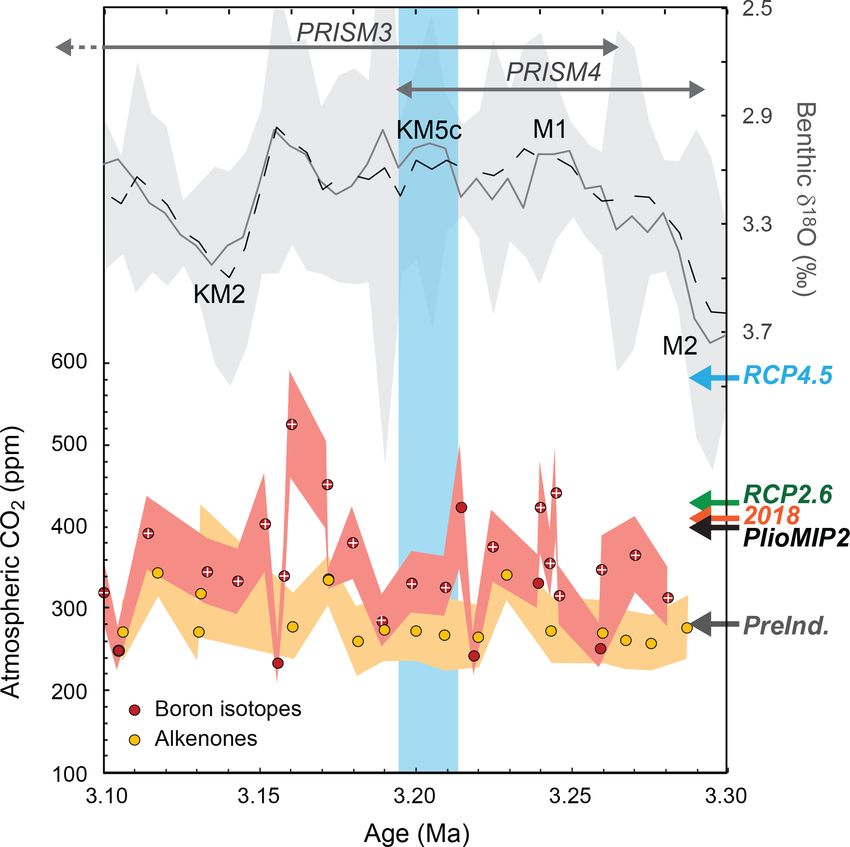
E. L. McClymont et al.: Lessons from a high-CO2 world                                                                           1601

                                                                      structed atmospheric CO2 concentrations from boron iso-
                                                                      topes in KM5c are 360±55 ppmv (for median boron-derived
                                                                      values (n = 3), full range: 289–502 ppmv, Fig. 1; Foster et
                                                                      al., 2017). A wider range of atmospheric CO2 concentrations
                                                                      has been reconstructed for the whole mid-Piacenzian stage
                                                                      (356 ± 65 ppmv for median values (n = 36), full range: 185–
                                                                      592 ppmv; Foster et al., 2017).

                                                                      2.2   Age models
                                                                      The PAGES-PlioVAR working group agreed on a set of
                                                                      stratigraphic protocols to maximise confidence in the iden-
                                                                      tification and analysis of orbital-scale variability within the
                                                                      mid-Piacenzian stage (McClymont et al., 2017). Sites were
                                                                      only included in the synthesis if they had either (i) ≤ 10 kyr
                                                                      resolution benthic δ 18 O data which could be (or had been)
                                                                      tied to the LR04 stack (Lisiecki and Raymo, 2005) or the
                                                                      HMM-Stack (Ahn et al., 2017) and/or (ii) the palaeomagnetic
                                                                      tie points for upper Mammoth (C2An.2n (b) at 3.22 Ma) and
                                                                      lower Mammoth (C2An.3n (t) at 3.33 Ma). At one site (ODP
                                                                      Site 1090) these conditions were not met (see Supplement),
Figure 1. The KM5c interglacial during the late Pliocene (3.195–      but tuning to LR04 had been made using a record of dust
3.215 Ma). Upper part of graph: benthic oxygen isotope stack (solid   concentrations under the assumption that higher dust flux
line: LR04, Lisiecki and Raymo, 2005; dashed line and grey shad-      occurred during glacials as observed during the Pleistocene
ing: Prob-stack mean and 95 % confidence interval, respectively,      (Martinez-Garcia et al., 2011). At ODP Site 806, uncertainty
Ahn et al., 2017). Selected Marine Isotope Stages (KM2 through        over age control resulted from the absence of an agreed splice
to M2) are highlighted. The KM5c interval of focus here is indi-      across the multiple holes drilled by ODP, and a new age
cated by the shaded blue bar. Previous Pliocene synthesis intervals   model has been constructed (see Supplement). For some sites
are also shown: PRISM3 (3.025–3.264 Ma) and PRISM4 (isotope           (see online summary at https://pliovar.github.io/km5c.html,
stages KM5c–M2; Dowsett et al., 2016). Lower part of graph: re-
                                                                      last access: 30 June 2020), revisions to the published age
constructed atmospheric CO2 concentrations (Foster et al., 2017).
                                                                      model were made, for example if the original data had been
Points show mean reported data (except white crosses: median val-
ues from Martinez-Boti et al., 2015); shading shows reported upper    published prior to the LR04 stack (Lisiecki and Raymo,
and lower estimates. Past and projected atmospheric CO2 concen-       2005) or prior to revisions to the palaeomagnetic timescale
trations highlighted by arrows: PlioMIP2 simulations are run with     (Gradstein et al., 2012). In total, data from 32 sites were com-
CO2 at 400 ppmv (Haywood et al., 2020) close to the annual mean       piled, extending from 46◦ S to 69◦ N (Fig. 2).
in 2018 (NOAA). Pre-industrial values from ice cores (Loulerge
et al., 2008) and projected representative concentration pathways     2.3   Proxy SST data
(RCP) for 2100 CE (IPCC, 2013).
                                                                      A multi-proxy approach was taken, to maximise the informa-
                                                                      tion available on changing climates and environments dur-
2     Methods                                                         ing the KM5c interval. Two SST proxies were analysed:
                                                                                                0
                                                                      the alkenone-derived UK  37 index (Prahl and Wakeham, 1987)
2.1    The KM5c interglacial                                          and foraminifera calcite Mg/Ca (Delaney et al., 1985). Both
                                                                      proxies have several calibrations to modern SST: here we ex-
KM5c (also referred to as KM5.3) is an interglacial centred
                                                                      plore the impact of calibration choice on KM5c SST data,
on a ∼ 100 kyr window of relatively depleted benthic 18 O
                                                                      by comparing and contrasting outputs between proxies and
values, which immediately follows a pronounced δ 18 O peak
                                                                      between calibrations. Although the TEX86 proxy (Schouten
during the glacial stage M2 (3.3 Ma; Fig. 1). Minor changes
                                                                      et al., 2002) has also been used to generate mid-Piacenzian
to orbital forcing during KM5 enables a wider target zone
                                                                      SSTs (e.g. O’Brien et al., 2014; Petrick et al., 2015; Rom-
(3.205 Ma ± 20 kyr) for data collection because the potential
                                                                      merskirchen et al., 2011), these data are not included here
for orbitally forced regional and time-transgressive climate
                                                                      because they could not be confidently assigned to the KM5c
signals is minimised (Haywood et al., 2013). A comparable
                                                                      interval either due to low sampling resolution and/or because
approach has been adopted by the PRISM4 synthesis (3.190
                                                                      our age control protocol was not met.
to 3.220 Ma; Foley and Dowsett, 2019; see Fig. 1). Here,
we focus on a narrow time slice from 3.195 to 3.215 Ma,
to span approximately one precession cycle. The recon-

https://doi.org/10.5194/cp-16-1599-2020                                                          Clim. Past, 16, 1599–1615, 2020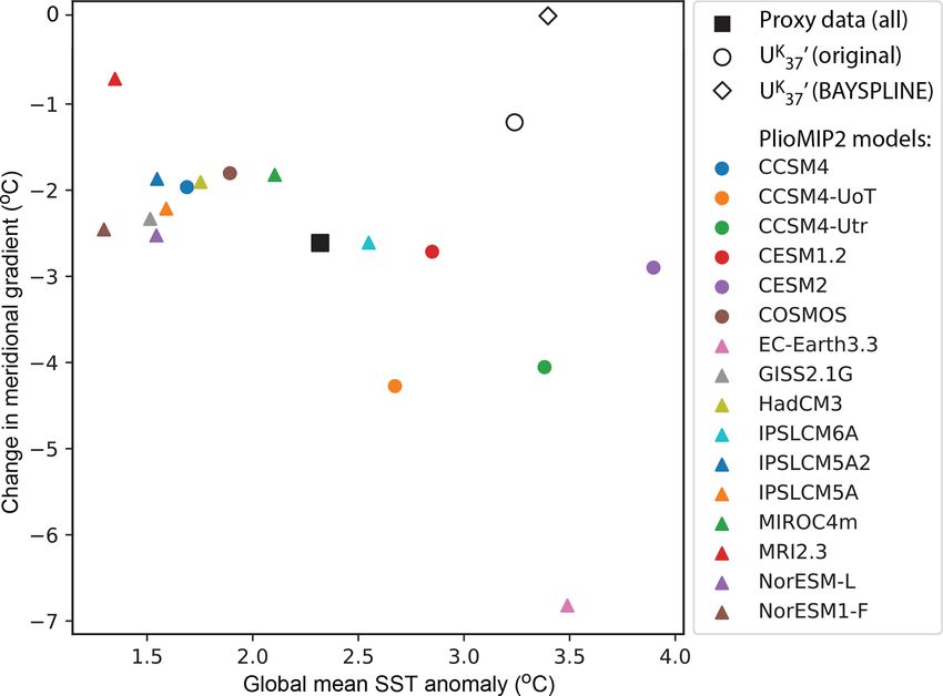
1602                                                                         E. L. McClymont et al.: Lessons from a high-CO2 world

Figure 2. Locations of sites used in the synthesis, overlain on mean annual SST data from the World Ocean Atlas 2018 (Locarnini et
                                                                                                     0
al., 2018). A full list of the data sources and proxies applied per site are available in Tables S3 (UK
                                                                                                      37 ) and S4 (Mg/Ca) in the Supplement and
can be accessed at https://pliovar.github.io/km5c.html (last access: 30 June 2020). The combined PlioVAR proxy data and their sources are
also archived at Pangaea: https://doi.pangaea.de/10.1594/PANGAEA.911847.

                                    0                                                        0
2.3.1   Alkenone SSTs (the UK
                            37
                               index)                                     converted all UK37 data to SSTs using both the Müller98 cal-
                                                                          ibration and the BAYSPLINE calibration. For most sites,
The majority of the 23 alkenone-derived SST datasets in-                  BAYSPLINE was run with the recommended setting for the
                                                  0
cluded in the PlioVAR synthesis used the UK      37 index and ap-         prior standard deviation scalar (pstd) of 10 (Tierney and Tin-
plied the linear core-top calibration (60◦ S–60◦ N) (Müller               gley, 2018). At high UK
                                                                                                   0                     ◦
                                                                                                 37 values (above ∼ 24 C) it is recom-
et al., 1998) (hereafter Müller98; Tables S2 and S3). The                 mended to use the more restrictive value of 5, to minimise
Müller98 calibration applies the best fit between core-top                the possibility of generating unrealistic SSTs (e.g. > 40 ◦ C)
    0
UK37 and modern SSTs, recorded at the sea surface (0 m                    given that the slope of the UK
                                                                                                          0
                                                                                                        37 –temperature calibration be-
water depth) and consistent with haptophyte productivity                  comes attenuated (Tierney and Tingley, 2018).
in the photic zone. The sedimentary signal is proposed
to record annual mean SST based on linear regression
                                                                          2.3.2    Foraminifera Mg/Ca
(Müller et al., 1998). Cultures of one of the dominant hapto-
phytes, Emiliania huxleyi, generated only minor differences               The magnesium-to-calcium ratio of foraminifera calcite can
                          0
in the slope of the UK   37 –temperature relationship (Table S2),         be used to reconstruct sea-surface (surface dwelling), ther-
where growth temperature was used for calibration (Prahl                  mocline (subsurface dwelling), and deep (benthic) ocean
et al., 1988). Several PlioVAR datasets were originally pub-              temperatures (Delaney et al., 1985; Elderfield et al., 1996;
lished using the Prahl et al. (1988) calibration (Table S3).              Rosenthal et al., 1997). The PlioVAR dataset includes anal-
   A recent expansion of the global core-top database (<                  ysis from 12 sites, on surface-dwelling foraminifera Glo-
70◦ N) was accompanied by Bayesian statistical analysis to                bigerinoides ruber, Trilobatus sacculifer, and Globigerina
                                                           0
assess the relationship(s) between predicted (from UK     37 ) and        bulloides (Table S4). In the original publications, data were
recorded ocean temperatures (Tierney and Tingley, 2018).                  converted to SST using a range of calibrations as well as
                 0
The revised UK  37 calibration, BAYSPLINE, addresses non-                 corrections for CaCO3 dissolution in the water column and
                       0
linearity in the UK  37 -SST relationship at the high end of              sediments, which leads to preferential removal of Mg from
the calibration, i.e. in the low-latitude oceans (Pelejero and            the CaCO3 lattice (generating cooler SSTs than expected;
Calvo, 2003; Sonzogni et al., 1997). BAYSPLINE also high-                 Dekens et al., 2002; Regenberg et al., 2006, 2009). The evo-
lights scatter between predicted and observed SSTs at the                 lution of the Mg/Ca of seawater (Mg/Caseawater ) over ge-
high latitudes and explicitly reconstructs seasonal SSTs >                ological timescales may also impact Mg/Ca-based palaeo-
45◦ N (Pacific) and > 48◦ N (Atlantic) and in the Mediter-                temperature reconstructions (Brennan et al., 2013; Coggon et
ranean Sea (Tierney and Tingley, 2018).                                   al., 2010; Fantle and DePaolo, 2005; Gothmann et al., 2015;
   To test the impact of different alkenone temperature cal-              Horita et al., 2002; Lowenstein et al., 2001). Changes in
ibrations on the quantification of mid-Piacenzian SSTs, we                Mg/Caseawater impact the intercept and potentially the sen-

Clim. Past, 16, 1599–1615, 2020                                                                  https://doi.org/10.5194/cp-16-1599-2020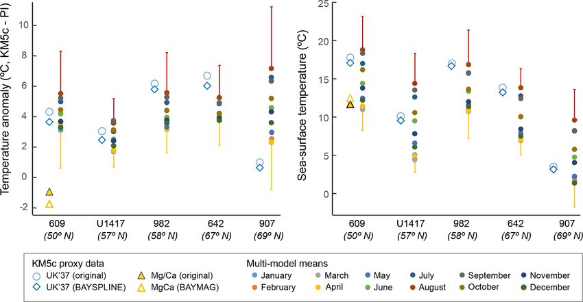
E. L. McClymont et al.: Lessons from a high-CO2 world                                                                           1603

sitivity of palaeotemperature equations (Evans and Müller,          sheet has no ice over West Antarctica. The reconstructed
2012; Medina-Elizalde and Lea, 2010), but there remains un-         PRISM4 ice sheets have a total volume of 20.1 × 10⁶ km3 ,
certainty over the magnitude of Mg/Caseawater changes in the        equating to a sea-level increase relative to the present day of
late Pliocene (O’Brien et al., 2014; Evans et al., 2016).           less than ∼ 24 m (Dowsett et al., 2016).
   To test the impact of different foraminifera Mg/Ca SST              Modelling groups had some choices regarding the exact
calibrations on mid-Piacenzian SSTs, we compare published           implementation of boundary conditions; however, 14 of the
SSTs with the recently developed BAYMAG calibration                 15 models used the “enhanced” PRISM4 boundary condi-
(Tierney et al., 2019b). We use published SSTs because              tions (Dowsett et al., 2016) which included all reconstructed
the original researchers used their best judgement to choose        changes to the land–sea mask and ocean bathymetry. Key
a particular Mg/Ca-SST calibration, given that it (i) fitted        ocean gateway changes relative to modern values are the
modern (regional) core-top values; (ii) accounted for known         closure of the Bering Strait and Canadian archipelago, and
environmental impacts (e.g. [CO2−  3 ] correction); (iii) was de-   the exposure of the Sunda and Sahul shelves (Dowsett et
veloped within a particular research group; and/or (iv) fitted      al., 2016). The initialisation of the experiments varied be-
conventional wisdom at the time. BAYMAG uses a Bayesian             tween models (Haywood et al., 2020). Some models were
approach that incorporates laboratory culture and core-top          initialised from a pre-industrial state while others were ini-
information to generate probabilistic estimates of past tem-        tialised from the end of a previous Pliocene simulation or
peratures. BAYMAG assumes a sensitivity of Mg/Ca to                 another warm state. The simulations reached equilibrium to-
salinity, pH, and saturation state at each core site and also       wards the end of the runs as per PlioMIP2 protocol.
accounts for Mg/Caseawater evolution through a linear scal-
ing (i.e. there is no change in the sensitivity of the palaeo-      2.5   Statistical analysis (calculating of global means and
temperature equation as Mg/Caseawater evolves) (Tierney et                meriodional gradients)
al., 2019b). For each site with Mg/Ca data, we computed
SSTs using BAYMAG’s species-specific hierarchical model.            For all anomaly calculations we obtain pre-industrial SST
In the absence of knowledge concerning changes in salin-            from the NOAA-ERSST5 dataset for the years 1870–
ity, pH, and saturation state in the Pliocene, we assumed that      1899 CE (Huang et al., 2017), ensuring alignment between
these values were the same as today. We drew seasonal sea-          the KM5c proxy data and the KM5c model experiments
surface salinity from the World Ocean Atlas 2013 product            (Haywood et al., 2020). This pre-industrial time window
(Boyer et al., 2013) and pH and bottom water saturation state       excludes the largest cooling linked to the Little Ice Age
from the GLODAPv2 product (Lauvset et al., 2016; Olsen et           and predates the onset of 20th-century warming (Owens et
al., 2016). We used a prior standard deviation of 6 ◦ C for all     al., 2017; PAGES2k Consortium, 2017). The global mean
sites.                                                              SST anomaly from the proxy data was obtained as follows:
                                                                    firstly, the SST anomaly between the proxy data and the
2.4   Climate models
                                                                    NOAA-ERSST5 data was obtained for each location and the
                                                                    data collated into bins of 15◦ of latitude. It is assumed that the
The model outputs used here were generated from the 15              average of all the data in each bin represents the average SST
models that contribute to the Pliocene modelling intercom-          anomaly for that latitude band. Next, the area of the ocean
parison project, Phase 2 (PlioMIP2) (Haywood et al., 2020).         surface for each bin is obtained. The average SST anomaly
The boundary conditions for the experiments and their large-        is then the average of all the bins weighted by the ocean area
scale results for Pliocene and pre-industrial climates are de-      in the relevant latitude band.
tailed elsewhere (Haywood et al., 2020, 2016b), so they are            Meridional gradients were obtained in a similar way. A
briefly outlined here.                                              low-latitude SST anomaly was obtained as the weighted av-
   The Pliocene simulations are intended to represent KM5c          erage of all the bins containing low-latitude SSTs (for exam-
(∼ 3.205 Ma) and were forced with PRISM4 boundary con-              ple the 4◦ × 15◦ bins containing latitudes of 30◦ S–30◦ N). A
ditions (Haywood et al., 2016b). Atmospheric CO2 concen-            high-latitude SST anomaly was obtained as the weighted av-
tration was set to 400 ppmv (Haywood et al., 2020), in line         erage of all bins containing high-latitude SSTs (> 60◦ N be-
with the upper estimates of atmospheric CO2 from boron              cause there were no proxy data points > 60◦ S). As only the
isotope data (Fig. 1; Foster et al., 2017). Lower estimates         Atlantic Ocean contained data points poleward of 65◦ N, the
from the alkenone carbon isotope proxy (Fig. 1) are likely          high-latitude region used in the gradient calculations for both
to reflect an insensitivity of this proxy to atmospheric CO2        proxies and models was focused on the longitudinal window
in the Pliocene (Badger et al., 2019). All other trace gases,       from 70◦ W to 5◦ E. The meridional gradient SST anomaly
orbital parameters, and the solar constant were specified to        is then the low-latitude SST anomaly minus the high-latitude
be consistent with each model’s pre-industrial experiment.          SST anomaly, relative to the pre-industrial period.
The Greenland Ice Sheet was confined to high elevations in             There are some uncertainties in this calculation of the
the eastern Greenland mountains, covering an area approxi-          global mean SST, in particular, the fact that the proxy data
mately 25 % of the present-day ice sheet. The Antarctic ice         are not evenly distributed throughout a latitude bin and also

https://doi.org/10.5194/cp-16-1599-2020                                                         Clim. Past, 16, 1599–1615, 2020
1604 E. L. McClymont et al.: Lessons from a high-CO2 world
that some bins contain very few data points. There is a higher higher than when using Müller98 (Fig. S2). The low-latitude
density of data in the Atlantic Ocean compared to the In- offset between Müller98 and BAYSPLINE has two effects: it
dian Ocean and Pacific Ocean, and no high-latitude data are elevates the global mean SST (Fig. 3, Table 1) and increases
available to consider a Southern Ocean response (Fig. 2). the KM5c meridional SST gradient towards pre-industrial
Nevertheless, this method of calculating averages does at- values (Figs. 3 and 4, Table 1). The calibration offsets are
tempt to account for unevenly distributed data and provides less systematic for Mg/Ca. There is a wider range of offsets
an SST anomaly (SSTA) that is comparable with model re- between BAYMAG and published SST values (from −4 to
sults. The impact of proxy choice was examined in the calcu- +5 ◦ C; Fig. S3, Table S3), although the smallest KM5c SST
lation of the global means and meridional SST gradients. As anomalies continue to be reconstructed in the low latitudes,
no Mg/Ca data were available > 50◦ N or > 30◦ S, we cal- regardless of which Mg/Ca calibration is applied (Fig. 4).
0
culated global mean SST and the meridional SST gradients Overall, the UK 37 –temperature anomalies lie within the
either including or excluding the Mg/Ca data; both results range given by PlioMIP2 models (Fig. 4). The Mg/Ca es-
are outlined below and shown in Table 1. timates are mainly from the low latitudes, and high-latitude
(> 60◦ N/S) Mg/Ca SST data are not available to calculate
meridional gradients using foraminifera data alone (Fig. 4).
0
3 Results Mg/Ca-SST anomalies are generally lower than for UK 37 , and
a cooler KM5c than the pre-industrial period is consistently
0
Relative to the pre-industrial period, the combined UK 37 and (but not always) recorded in the low latitudes by Mg/Ca re-
Mg/Ca proxy data, using the original calibrations, indicate gardless of calibration choice (Fig. 4). As a result, combining
0
a KM5c global mean SST anomaly of +2.3 ◦ C and a merid- UK37 and Mg/Ca data leads to a cooler global mean SST (∼
ional SST gradient reduced by 2.6 ◦ C (Fig. 3). The amplitude 2.3 ◦ C) than when using U37 K0 alone (∼ 3.2 ◦ C with Müller98,
of the global SST mean anomaly in the combined proxy data ∼ 3.4 ◦ C with BAYSPLINE; Fig. 3 and Table 1). At eight
exceeds those indicated in 10 of the PlioMIP2 models but sites, the negative KM5c SST anomalies in Mg/Ca disagree
0
is lower than the global SST anomaly from 6 models. The with both the UK 37 data and the PlioMIP2 model outputs
meridional temperature gradient anomalies are more compa- (Fig. 4). The disagreement is present regardless of whether
0
rable (Fig. 3). If only the UK
37 data are used, the global mean the Müller98 or BAYSPLINE calibrations are applied, but
SST anomaly from proxies is higher than all but three of the difference is larger in the low latitudes for BAYSPLINE
0
the PlioMIP2 models, and the UK 37 meridional gradient cal- because here this calibration generates higher SST values
0
culations are smaller than all models (BAYSPLINE) or one (Sect. 2.3.1). Only three sites have both UK 37 and Mg/Ca
model (original calibration; Fig. 3). data (DSDP Site 609, IODP sites U1313 and U1143) to en-
Overall, the proxy data show the lowest temperature able direct comparison between Mg/Ca and alkenone SST
anomalies in the low latitudes, regardless of proxy (from +3 data. Reconstructed SSTs for IODP sites U1313 and U1143
to −4 ◦ C for sites < 30◦ N/S). A larger range of temperature are within calibration uncertainty. At Site U1313 (41◦ N)
anomalies is reconstructed in the mid-latitudes and high lati- there is overlap between both alkenone outputs (Müller98
tudes (from +9 to −2 ◦ C for sites > 30◦ N/S) (Fig. 4). Thus, 21.6 ◦ C, BAYSPLINE 20.9 ◦ C) and the original Mg/Ca re-
there is a broad, but complex, pattern of enhanced warming at construction (22.2 ◦ C), whereas BAYMAG generates warmer
the mid-latitudes and high latitudes, reflecting a combination SSTs (27.0 ◦ C). At Site 1143 (9◦ N), BAYSPLINE SSTs are
of regional influences on circulation patterns and, to some ex- warmer (30.6 ◦ C) than from the Müller98 (28.9 ◦ C), origi-
tent, proxy choice. This pattern is not explained by temporal nal Mg/Ca (27.7 ◦ C), and BAYMAG (27.1 ◦ C) calibrations.
variability nor sample density within the KM5c time interval: In contrast, DSDP Site 609 (49◦ N) has colder Mg/Ca esti-
regardless of sample number per site, the standard deviation mates (original 11.7 ◦ C, BAYMAG 12.5 ◦ C) than alkenones
at any site within the KM5c time bin is < 1.5 ◦ C (Fig. S4 (Müller98 17.7 ◦ C, BAYSPLINE 17.1 ◦ C) or models (Fig. 4).
in the Supplement). We note that of the 32 sites examined
here, 7 provided a single data point for the KM5c interval
4 Discussion
(Fig. S2, alkenones: ODP Sites 907, 1081, U1337, U1417;
Fig. S3, foraminifera Mg/Ca: DSDP sites 214, 709, 763);
4.1 SST expression of the KM5c interglacial
the sites are geographically well distributed, however, and
so unlikely to significantly impact our global mean/gradient KM5c is characterised by a surface ocean which is ∼ 2.3 ◦ C
calculations. (alkenones and Mg/Ca), ∼ 3.2 ◦ C (alkenones-only, Müller98
Calibration choice has a small impact over the recon- calibration), or ∼ 3.4 ◦ C (alkenones-only, BAYSPLINE cal-
structed patterns of KM5c SST anomalies (Figs. 4, S2, ibration) warmer than pre-industrial values, with a ∼ 2.6 ◦ C
0
and S3). Below 24 ◦ C, absolute UK 37 SSTs using Müller98 are reduction in the meridional SST gradient. The global mean
◦
< 1 C lower than those using BAYSPLINE. At high tem- SST anomaly is higher than the 1.7 ◦ C previously calculated
peratures the non-linearity in the BAYSPLINE calibration for the wider mid-Piacenzian warm period (3.1–3.3 Ma), re-
means that BAYSPLINE SSTs can be up to 1.67 ◦ C±0.01 ◦ C gardless of proxy choice (IPCC, 2014b). Previous analysis
Clim. Past, 16, 1599–1615, 2020 https://doi.org/10.5194/cp-16-1599-2020E. L. McClymont et al.: Lessons from a high-CO2 world 1605
Table 1. Comparison of the magnitude of the global SST anomaly and meridional SST gradients between KM5c and the pre-industrial
period, depending on proxy combination, and the latitudinal bands used for the gradient calculations.
Proxy Global mean SST Meridional SST gradient
anomaly, ◦ C anomaly, ◦ C
30◦ S–30◦ N minus 0–30◦ N minus 15◦ S–15◦ N minus
> 60◦ N > 60◦ N > 45◦ N/S
0
UK
370 (original) 3.24 −1.18 −3.00 −1.56
UK
370 (BAYSPLINE) 3.41 0.03 −1.66 −0.18
UK
370 (original) + Mg/Ca 2.32 −2.61 −4.08 −2.84
UK
37 (BAYSPLINE) + Mg/Ca (BAYMAG) 2.28 −2.21 −3.13 −2.19
Figure 3. Comparison of KM5c SST data relative to the pre-industrial period (NOAA-ERSST5) for global mean SST anomalies (SSTA) and
the change in meridional SST gradient, constructed using proxy data and the suite of PlioMIP2 models. Details of the model experiments
are outlined in Table 1 of Haywood et al. (2020). The meridional SST gradient is calculated as 30◦ S–30◦ N minus 60–75◦ N, so that a more
negative change in the gradient reflects a larger warming anomaly at high latitudes relative to low latitudes. As we only had data points
poleward of 65◦ N in the Atlantic Ocean, the high-latitude region for both proxy and model gradient calculations focuses on the longitudinal
0
window from 70◦ W to 5◦ E. Proxy data calculations were made using either all proxy data (UK 37 and Mg/Ca using their original calibrations)
0
or using only UK ◦
37 data and comparing the original and BAYSPLINE calibrations. No Mg/Ca data are available > 60 N, so we were unable
to calculate Mg/Ca-only gradients (Fig. 4). The impact of changing the low- and high-latitude bands is explored in Table 1.
of a suite of models suggested that a climate state resem- els when we use only alkenones or alkenones and Mg/Ca
bling the mid-Piacenzian was likely to develop and be sus- combined (Fig. 3), and hence our results suggest that the
tained under RCP4.5 (Burke et al., 2018). The PlioMIP2 global annual surface air temperature anomaly for KM5c
ensemble (Haywood et al., 2020) indicates that best es- would exceed the PlioMIP2 multi-model surface air temper-
timates for mid-Piacenzian warming in surface air tem- ature mean of 2.8 ◦ C (Haywood et al., 2020). The higher
peratures (1.7–5.2◦ ) are comparable to projections for the global SST mean recorded in the KM5c proxy data, com-
RCP4.5 to 8.5 scenarios by 2100 CE (RCP4.5 = 1.8 ± 0.5◦ , pared to the PlioMIP2 models, occurs despite the available
RCP8.5 = 3.7±0.7 ◦ C; IPCC, 2013). Our proxy-based mean atmospheric CO2 reconstructions indicating values below the
global SST anomaly is larger than in most PlioMIP2 mod- ∼ 400 ppmv used in the PlioMIP2 models (Fig. 1). Our syn-
https://doi.org/10.5194/cp-16-1599-2020 Clim. Past, 16, 1599–1615, 20201606 E. L. McClymont et al.: Lessons from a high-CO2 world
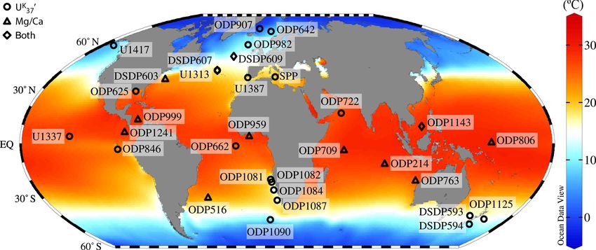
Figure 4. Reconstructed and modelled SST anomalies plotted by latitude. SST reconstructions using the original published data and two
Bayesian approaches (BAYSPLINE, BAYMAG) are shown. The anomalies are calculated with reference to the NOAA-ERSST5 data for the
years 1870–1899 CE at each site. Vertical red lines show the range of modelled annual SSTs from all PlioMIP2 experiments (Haywood et
al., 2020) calculated at the grid boxes containing each site.
thesis of SST data thus indicates that with atmospheric CO2 eral (but not all) low-latitude sites recording negative SST
concentrations ≤ 400 ppmv (comparable to RCP4.5), the sur- anomalies for KM5c using foraminifera Mg/Ca, the in-
face ocean warming response will likely be larger than in- clusion of Mg/Ca data leads to a larger difference in the
dicated in models. Further work is required to increase the meridional SST gradient relative to the pre-industrial period
temporal resolution of the atmospheric CO2 reconstructions (−2.19 to −4.08 ◦ C). Further work is required to fully under-
through KM5c, to improve our understanding of the recon- stand the negative KM5c SST anomalies in some of the low-
structed SST response to CO2 forcing, including whether (or latitude sites (discussed further below), given their impact
by how much) the reconstructed atmospheric CO2 differs on the meridional SST gradients. However, a robust pattern
from model boundary conditions and whether other changes emerging from the data is that the KM5c proxy data detail
in the model boundary conditions also influence SST patterns smaller low-latitude SST anomalies than those of the mid-
(e.g. gateway changes outlined in Sect. 2.4). and high-latitude SST anomalies (Fig. 4), leading to a re-
Proxy choice, calibration choice, and site selection have duction in the meridional SST gradient relative to the pre-
all had an impact on the magnitude of the change in merid- industrial period. Enhanced mid- and high-latitude warming
ional SST gradient for KM5c compared to the pre-industrial has been observed in other warm intervals of the geological
period (Table 1). Focussing only on a Northern Hemisphere past, including the last interglacial and the Eocene (Evans et
SST gradient leads to higher gradient anomalies than when al., 2018; Fischer et al., 2018), and is a feature of future cli-
all of the low latitudes are included (30◦ S–30◦ N) because it mate under elevated CO2 concentrations (IPCC, 2014a).
excludes the high SST anomalies of the Benguela upwelling There is complexity in the amplitude of the KM5c SST
sites (20–25◦ S; discussed below, Fig. 4). Smaller meridional anomaly by latitude and basin, which may reflect patterns of
SST gradient anomalies occur using BAYSPLINE (+0.03 to surface ocean circulation. In the Northern Hemisphere, rela-
0
−1.66 ◦ C) than the Müller98 calibration for UK 37 (−1.18 to tively muted warming in the East Greenland Current (ODP
−3.00 ◦ C; Table 1), due to the increased low-latitude SST Site 907, 69◦ N) may reflect the presence of at least seasonal
anomalies generated by BAYSPLINE (Fig. 4). Due to sev- sea-ice cover from ca. 4.5 Ma (Clotten et al., 2018). In con-
Clim. Past, 16, 1599–1615, 2020 https://doi.org/10.5194/cp-16-1599-2020E. L. McClymont et al.: Lessons from a high-CO2 world 1607
trast, relatively high SST anomalies at ODP Sites 642 (67◦ N) 4.2 Proxy data–model comparisons for mid- and
and 982 (58◦ N) track the northward flow of the North At- high-latitude sites
lantic Current, accounting for the enhanced warming rela-
tive to north-east Pacific IODP Site U1417 (57◦ N; Figs. 4 For the mid-latitudes and high latitudes, we find broad proxy
and 5). The large North Atlantic SST anomalies also con- data–model agreements for most sites. In the North Atlantic
0
tribute to an enhanced Northern Hemisphere meridional SST Ocean, reconstructed SST KM5c anomalies from UK 37 fall
gradient of up to 4 ◦ C (> 60◦ N minus 0–30◦ N; Table 1). within the ranges provided by the PlioMIP2 models (Fig. 4)
For the Southern Hemisphere, a signal of polar amplification for all but one site (IODP Site U1387, 37◦ N). The over-
0
is less clearly identified than for the Northern Hemisphere all UK37 –model agreement for the North Atlantic Ocean sug-
(Fig. 4), although we recognise that all sites are 45◦ N (Tierney
and Tingley, 2018). Despite these differences in interpreta-
tion, BAYSPLINE values for KM5c are < 0.7 ◦ C cooler than
https://doi.org/10.5194/cp-16-1599-2020 Clim. Past, 16, 1599–1615, 20201608 E. L. McClymont et al.: Lessons from a high-CO2 world
Figure 5. Investigating the potential seasonal signature recorded at high-latitude Northern Hemisphere sites (> 50◦ N), ordered by increasing
latitude from left to right. Note that Site U1417 is from the North Pacific, where BAYSPLINE explicitly assumes that a summer signal is
recorded > 48◦ N. All other sites are from the Atlantic Ocean/Nordic Seas, where BAYSPLINE assumes an autumn signal > 45◦ N. The
original calibration by Müller et al. (1998) proposes that mean annual SSTs are recorded. Standard deviations of the multi-model means are
shown for August (red) and April (yellow), which tend to be the maxima and minima, respectively.
0
the original published UK 37 data (Fig. S2). Although the North the Pliocene (as reconstructed in the equatorial Pacific (Ford
K 0
Atlantic U37 data align with a range of mean annual SST and Ravelo, 2019; Ford et al., 2015; Steph et al., 2006; Steph
anomalies generated by the PlioMIP2 models (Fig. 4), three et al., 2010) and theorised globally (Philander and Fedorov,
0
of the sites show alignment between UK 37 SSTs and the July–
2003)), so that warmer subsurface waters than today were
November values from the multi-model means (Fig. 5). In upwelled, enhancing local warming. However, warming of
contrast, Site 907 aligns with cool spring temperatures in the ∼ 3.4 ◦ C in subsurface waters (Ford and Ravelo, 2019) and
models, perhaps reflecting production after sea ice melt. ∼ 2.5 ◦ C in intermediate waters (McClymont et al., 2016)
The large data–model discrepancy at 30◦ S reflects three for Pliocene interglacials suggests that Pliocene upwelling of
sites which today sit beneath the Benguela upwelling system warmer waters is unable to fully account for the 7–10 ◦ C SST
in the south-east Atlantic (20–26◦ S; Fig. 4). Part of the data– anomalies at Benguela sites for KM5c. Changes to the distri-
model discrepancy in the KM5c anomaly can be attributed to bution of export productivity and SSTs indicate that an over-
the models overestimating pre-industrial SSTs at the north- all poleward displacement of the Benguela upwelling system
ern Benguela sites (NOAA-ERSST5 SSTs are 2–5 ◦ C be- occurred during the Pliocene, so that the main zone of up-
low the pre-industrial model range) and suggests that mod- welling likely sat close to ODP Site 1087 at 31◦ S (Etourneau
els are not fully capturing the local dynamics of the coastal et al., 2009; Petrick et al., 2018; Rosell-Melé et al., 2014). As
upwelling today (Small et al., 2015). Realistic representa- the northern and southern Benguela regions are today marked
tions of the Benguela upwelling system today are proposed by differences in the seasonality of the upwelling, a temporal
to require realistic wind stress curl and high-resolution atmo- shift in upwelling intensity may also account for some of the
sphere and ocean models (< 1◦ ; Small et al., 2015). Most of large SST anomaly (Haywood et al., 2020). Thus, the data–
the PlioMIP2 simulations use lower-resolution atmosphere model disagreement may be accounted for by a combination
and ocean models (Haywood et al., 2020). An increased den- of displaced upwelling and warmer upwelled waters, giving
sity of proxy data reconstructing KM5c atmospheric circu- large SST anomalies in Benguela proxy data, alongside the
lation, as well as the application of high-resolution models, challenges of modelling both the pre-industrial and KM5c
may help to understand the observed KM5c data–model dis- upwelling system and its associated SSTs.
crepancy. Furthermore, there was a deep thermocline during Data–model disagreement also occurs at two Northern
0
Hemisphere sites where UK 37 -SST anomalies exceed those
Clim. Past, 16, 1599–1615, 2020 https://doi.org/10.5194/cp-16-1599-2020E. L. McClymont et al.: Lessons from a high-CO2 world 1609
given by the range of model predictions (Fig. 4). Punto Pic- for ODP Site 806 in the western Pacific warm pool, BAY-
cola (Sicily, 37◦ N) is located within the Mediterranean Sea, MAG SST estimates for KM5c are ∼ 1 ◦ C warmer than the
whereas IODP Site U1387 (37◦ N, Iberian margin) records published Mg/Ca record (Wara et al., 2005). For Site 999
the influence of the waters sourced from the Azores Current in the Caribbean Sea, BAYMAG SST estimates for KM5c
and the subtropical gyre. The data–model disagreement for are ∼ 0.5 ◦ C cooler than the published Mg/Ca record (De
KM5c reflects warmer SST estimates from the proxy data Schepper et al., 2013). This also suggests that the impact of
compared to the models, despite the good agreement for the Mg/Caseawater change on SST is small on warm pool sites.
pre-industrial period suggesting that locally complex ocean The Mg/Caseawater correction used in BAYMAG is conserva-
circulation in these near-shore and marginal marine settings tive, drawing on multiple lines of physical evidence (corals,
may have been captured in the models. For Punto Piccola, fluid inclusions, calcite veins, etc.) (Tierney et al., 2019b).
the data–model offset is also likely to be a minimum be- Given the variable directions of the offsets between pub-
cause BAYSPLINE Mediterranean SSTs explicitly record lished and BAYMAG SSTs shown here, the Mg/Caseawater
November–May temperatures (Tierney and Tingley, 2018), correction is unable to account for the data–model offsets ob-
and alkenone production below the sea surface has also been served for the low latitudes.
proposed (Ternois et al., 1997): both scenarios would act to CaCO3 dissolution in the water column and sediments
raise mean annual SSTs further from those simulated in the could lead to a cool bias on the Mg/Ca SSTs (Dekens et
PlioMIP2 models (Fig. 4). Further multi-proxy investigation al., 2002; Regenberg et al., 2006, 2009). However, the cool
is required to identify whether the data–model disagreements KM5c anomalies also occur if the forward-modelled core-top
in the Benguela upwelling, Gulf of Cadiz, and Mediterranean Mg/Ca SSTs from BAYMAG are used as the pre-industrial
Sea reflect challenges in modelling near-shore or complex “reference” (Fig. S6). The cold low-latitude anomalies for
oceanographic systems and/or biases in the temperature sig- KM5c could reflect an increase in the calcification depth
nal recorded by the proxy data. of the foraminifera, since the surface-dwelling foraminifera
analysed here calcify at a range of depths, particularly in the
4.3 Data–model comparisons for low-latitude sites tropics where the thermocline is deep in comparison to mid-
0
latitudes to high latitudes (Fairbanks et al., 1982; Curry et
The low-latitude UK 37 -SST anomalies for KM5c align well al., 1983). The negative anomalies are broadly smaller for
with the PlioMIP2 models (Fig. 4). At ODP Sites 806 and G. ruber (−0.4 to −1.2 ◦ C) than for T. sacculifer (−0.6 to
959, the Mg/Ca anomalies using the original calibrations are −3.5 ◦ C), consistent with a deeper depth habitat for the lat-
both +0.3 ◦ C compared to the pre-industrial period (Fig. 4) ter (Curry et al., 1983), although at Site 959 the G. ruber
and also align with the PlioMIP2 models. At Site 806 the anomaly using BAYMAG is −3.8 ◦ C. There is therefore a
BAYMAG KM5c anomaly (+1.7 ◦ C) also aligns with the lack of consistency between sites, which is difficult to re-
0
PlioMIP2 models. Only one low-latitude site has both UK 37 solve when single species have been analysed for each of the
and Mg/Ca SST data: ODP Site 1143 (9◦ N) records KM5c sites through KM5c.
0
anomalies of +0.8 to +2.5 ◦ C (UK 37 ) or −0.7 to −1.3 C
◦
Where there are very large differences between BAYMAG
K 0
(Mg/Ca). Although the U37 data align with the model out- and published Mg/Ca SST estimates, regardless of latitude
puts for Site 1143, the negative anomaly in Mg/Ca lies out- (e.g. North Atlantic; Fig. 4), we suggest that some combina-
side the model range for mean annual SST (Fig. 4). tion of calibration difference, Mg/Caseawater change, and/or
Six of the low-latitude sites have negative low-latitude other environmental factors including seasonality and cal-
SST anomalies in KM5c from foraminifera Mg/Ca; these cification depth may offer an explanation. To fully investi-
occur regardless of whether the original or BAYMAG cali- gate the cause(s) of offsets in Mg/Ca SST reconstructions
brations are applied and for both G. ruber and T. sacculifer- requires future multi-species analysis for Mg/Ca for each
based reconstructions. The negative KM5c Mg/Ca-SST site and multi-proxy analysis for each site. Such an approach
anomalies lie beyond those shown across the PlioMIP2 would enable the exploration of a wider range of potential
0
model range (Fig. 4), despite the absolute Mg/Ca SSTs re- influences over both the Mg/Ca and UK 37 -SST reconstruc-
constructed from these sites for KM5c falling within the tions and a reduction in the uncertainties of the reconstructed
model range for all but two of the sites (ODP Sites 999 SSTs and their anomalies. Alongside foraminifera Mg/Ca
0
(13◦ N) and 1241 (6◦ N); Fig. S5). However, the absolute and UK 37 analyses, additional proxies which are likely to add
SST values reconstructed for KM5c from Mg/Ca tend to valuable information about water column structure and sea-
align with the colder model outputs (Fig. S5). sonality could include TEX86 (Schouten et al., 2002), long-
Mg/Ca-SST calibration choice has no consistent impact chain diols (Rampen et al., 2012), and clumped isotopes (Tri-
on the KM5c anomalies (across all latitudes; Fig. 4). There- pati et al., 2010). Previous research has demonstrated that
fore, the corrections for secular seawater Mg/Ca change even within a single site there can be offsets between proxies
and/or non-thermal influences over Mg/Ca, which are ac- which are not continuous through time (e.g. Lawrence and
counted for in BAYMAG (Tierney et al., 2019b), do not ac- Woodard, 2017; Petrick et al., 2018), so that high-resolution
count for these cold tropical KM5c anomalies. For example, and multi-proxy work is required to fully understand the off-
https://doi.org/10.5194/cp-16-1599-2020 Clim. Past, 16, 1599–1615, 20201610 E. L. McClymont et al.: Lessons from a high-CO2 world
sets we have identified here. Resolving the causes of the dif- relative to the pre-industrial period. More data points are re-
ferent proxy–proxy and proxy–model offsets is important be- quired to fully explore these patterns: for seven sites only
cause they impact the calculation of the global mean SST one data point lay within KM5c, and more than half of the
anomaly relative to pre-industrial values; however, even with analysed sites (18/32) recorded Atlantic Ocean SSTs.
the inclusion of the overall cooler Mg/Ca data, the combined Both the PlioMIP2 models (Haywood et al., 2020) and fu-
KM5c proxy data still indicate a global mean SST anomaly ture projections (IPCC, 2019) indicate that warming is higher
which is larger than most models from the PlioMIP2 experi- over land than in the oceans in response to higher atmo-
ments (Fig. 3). spheric CO2 concentrations. Our synthesis of KM5c thus
likely represents a minimum warming to be expected with
atmospheric CO2 concentrations of ∼ 400 ppmv. Even un-
5 Conclusions der low-CO2 emission scenarios, our results demonstrate that
surface ocean warming may be expected to exceed model
This study has generated a new multi-proxy synthesis of SST projections and will be accentuated in the higher latitudes.
data for an interglacial stage (KM5c) from the Pliocene. By
selecting an individual interglacial, with orbital forcing sim-
ilar to modern values, we are able to focus on the SST re- Data availability. The combined proxy data (absolute SST
sponse to atmospheric CO2 concentrations comparable to to- reconstructions and anomalies to the pre-industrial pe-
day and the near future (∼ 400 ppmv) but elevated relative riod) and full details of the data sources are available at
to the pre-industrial period. Using strict stratigraphic proto- https://doi.org/10.1594/PANGAEA.911847 (McClymont et al.,
2020).
cols we selected only those data which could be confidently
aligned to KM5c. By comparing different calibrations and
0
two different proxy systems (UK 37 and Mg/Ca in planktonic Supplement. Additional information on proxy calibrations and
foraminifera) we identified several robust signals which are their impact on the SST reconstructions is available in the sup-
proxy-independent. First, global mean SSTs during KM5c plement. The supplement related to this article is available online
were warmer than pre-industrial values. Second, there was a at: https://doi.org/10.5194/cp-16-1599-2020-supplement.
reduced meridional SST gradient which is the result of rela-
tively small low-latitude SST anomalies and a larger range of
warming anomalies for the mid-latitudes and high latitudes. Author contributions. ELM, HLF, and SLH designed the data
Overall, there is good data–model agreement for both the ab- analysis and led the data compilation. JCT and AMH processed
solute SSTs and the anomalies relative to the pre-industrial outputs from the suite of PlioMIP2 models, and calculated global
period, although there are complexities in the results. Further means and meridional SST gradients using the proxy data. Proxy
work is required to generate multi-proxy SST data from sin- data were compiled and their age models reviewed by ELM, HLF,
gle sites, accompanied by robust reconstructions of thermo- MAG, IB, KL, MP, BP, ACR, BR, SDS, GEAS, KT, and SW. Proxy
cline temperatures using multi-species foraminifera analysis, calibrations were reviewed and applied by ELM, MAB, HLF, SLH,
FP, JET, and CvdW. PlioMIP2 model experiments were designed
so that the range of factors explaining proxy and calibration
and run and the outputs processed by AAO, MLJB, EB, WLC, DC,
offsets can be explored more fully. RF, CG, AMH, AvdH, SH, XL, GL, KHN, BLOB, WRP, CS, JCT,
The choice of proxy for SST reconstruction impacts the and ZZ. ELM, HLF, and SLH prepared the paper with contributions
overall calculation of global mean SST and the meridional from all co-authors.
gradients. The negative anomalies in Mg/Ca SSTs at 6 of the
16 low-latitude sites lowers the global mean SST of KM5c
0 K0
from ∼ 3.2–3.4 ◦ C (UK ◦
37 -only) to ∼ 2.3 C (combined U37 Competing interests. The authors declare that they have no con-
and Mg/Ca). The meridional SST gradient anomalies are de- flict of interest.
0
creased to −2.6 ◦ C (combined UK 37 and Mg/Ca) relative to
the pre-industrial period, although a more muted reduction
0
(up to −1.18◦ C) occurs with UK 37 alone. A number of factors Special issue statement. This article is part of the special issue
may lead to a cool bias in the foraminifera Mg/Ca SSTs, “PlioMIP Phase 2: experimental design, implementation and scien-
which require further investigation through multi-proxy and tific results”. It is not associated with a conference.
multi-species analysis, particularly at low-latitude sites.
We identify the strongest warming across the North At-
lantic region. The results are consistent with the PlioMIP2 Acknowledgements. This work is an outcome from several
0 workshops sponsored by Past Global Change (PAGES) as con-
models, although the largely UK 37 data sit at the high end of tributions to the working group on Pliocene Climate Vari-
the calculated model anomalies. Although seasonality may
ability over glacial-interglacial timescales (PlioVAR). We ac-
play a role in the proxy data signal, these results also suggest knowledge PAGES for their support and the workshop partici-
that many models may underestimate high-latitude warming pants for discussions. Funding support has also been provided
even with the moderate CO2 increases identified in KM5c
Clim. Past, 16, 1599–1615, 2020 https://doi.org/10.5194/cp-16-1599-2020E. L. McClymont et al.: Lessons from a high-CO2 world 1611
by NERC (NE/I027703/1 and NE/L002426/1 to Erin L. Mc- References
Clymont, NERC NE/N015045/1 to Heather L. Ford), Lever-
hulme Trust (Philip Leverhulme Prize, Erin L. McClymont), Ahn, S., Khider, D., Lisiecki, L. E., and Lawrence, C.
and the Research Council of Norway (Bjørg Risebrobakken and E.: A probabilistic Pliocene–Pleistocene stack of ben-
Erin L. McClymont (221712), Stijn De Schepper (229819)). thic δ18O using a profile hidden Markov model, Dy-
Michiel L. J. Baatsen, Anna von der Heydt, Francien Pe- namics and Statistics of the Climate System, 2, dzx002,
terse, and Carolien van der Weijst are part of the Nether- https://doi.org/10.1093/climsys/dzx002, 2017.
lands Earth System Science Centre (NESSC), financially sup- Badger, M. P. S., Chalk, T. B., Foster, G. L., Bown, P. R., Gibbs,
ported by the Dutch Ministry of Education, Culture and Science S. J., Sexton, P. F., Schmidt, D. N., Pälike, H., Mackensen, A.,
(OCW). Montserrat Alonso-Garcia acknowledges support from and Pancost, R. D.: Insensitivity of alkenone carbon isotopes to
FCT (SFRH/BPD/96960/2013, PTDC/MAR-PRO/3396/2014, and atmospheric CO2 at low to moderate CO2 levels, Clim. Past, 15,
CCMAR UID/Multi/04326/2019). W. Richard Peltier and Deepak 539–554, https://doi.org/10.5194/cp-15-539-2019, 2019.
Chandan were supported by Canadian NSERC Discovery Grant Bolton, C. T., Bailey, I., Friedrich, O., Tachikawa, K., de Garidel-
A9627, and they wish to acknowledge the support of SciNet HPC Thoron, T., Vidal, L., Sonzogni, C., Marino, G., Rohling, E. J.,
Consortium for providing computing facilities. SciNet is funded Robinson, M. M., Ermini, M., Koch, M., Cooper, M. J., and
by the Canada Foundation for Innovation under the auspices of Wilson, P. A.: North Atlantic Midlatitude Surface-Circulation
Compute Canada, the Government of Ontario, the Ontario Re- Changes Through the Plio-Pleistocene Intensification of North-
search Fund – Research Excellence, and the University of Toronto. ern Hemisphere Glaciation, Paleoceanography and Paleoclima-
Gerrit Lohmann and Christian Stepanek acknowledge funding by tology, 33, 1186–1205, https://doi.org/10.1029/2018pa003412,
the Helmholtz Climate Initiative REKLIM and the Alfred We- 2018.
gener Institute’s research programme PACES2. Wing-Le Chan Boyer, T. P., Antonov, J. I., Baranova, O. K., Coleman, C., Gar-
and Ayako Abe-Ouchi acknowledge funding from JSPS KAK- cia, H. E., Grodsky, A., Johnson, D. R., Locarnini, R. A., Mis-
ENHI grant 17H06104 and MEXT KAKENHI grant 17H06323 honov, A. V., O’Brien, T. D., Paver, C. R., Reagan, J. R., Seidov,
as well as JAMSTEC for use of the Earth Simulator supercom- D., Smolyar, I. V., and Zweng, M. M.: World Ocean Database
puter. Bette L. Otto-Bliesner, Esther C. Brady, and Ran Feng ac- 2013, in: NOAA Atlas NESDIS 72, edited by: Levitus, S. and
knowledge the CESM project, which is supported primarily by Mishonov, A., National Oceanic and Atmospheric Administra-
the National Science Foundation (NSF). This material is based tion Ocean Climate Laboratory, Silver Spring, MD, 209 pp.,
upon work supported by the National Center for Atmospheric https://doi.org/10.7289/V5NZ85MT, 2013.
Research (NCAR), which is a major facility sponsored by the Brennan, S. T., Lowenstein, T. K., and Cendón, D. I.: The major-
NSF under Cooperative Agreement No. 1852977. Computing and ion composition of Cenozoic seawater: The past 36 million years
data storage resources, including the Cheyenne supercomputer from fluid inclusions in marine halite, Am. J. Sci., 313, 713–775,
(https://doi.org/10.5065/D6RX99HX), were provided by the Com- https://doi.org/10.2475/08.2013.01, 2013.
putational and Information Systems Laboratory (CISL) at NCAR. Burke, K. D., Williams, J. W., Chandler, M. A., Hay-
This research used samples and/or data provided by the Interna- wood, A. M., Lunt, D. J., and Otto-Bliesner, B. L.:
tional Ocean Discovery Program (IODP), Ocean Drilling Program Pliocene and Eocene provide best analogs for near-future
(ODP), and Deep Sea Drilling Project (DSDP). climates, P. Natl. Acad. Sci. USA, 115, 13288–13293,
https://doi.org/10.1073/pnas.1809600115, 2018.
Caballero-Gill, R. P., Herbert, T. D., and Dowsett, H. J.: 100-kyr
Financial support. This research has been supported by Paced Climate Change in the Pliocene Warm Period, Southwest
the NERC (grant nos. NE/I027703/1, NE/L002426/1, and Pacific, Paleoceanography and Paleoclimatology, 34, 524–545,
NE/N015045/1), the Leverhulme Trust, the Research Council https://doi.org/10.1029/2018pa003496, 2019.
of Norway (grant nos. 221712 and 229819), the Dutch Min- Clotten, C., Stein, R., Fahl, K., and De Schepper, S.: Seasonal sea
istry of Education, Culture and Science (OCW), FCT (grant ice cover during the warm Pliocene: Evidence from the Ice-
nos. SFRH/BPD/96960/2013, PTDC/MAR-PRO/3396/2014, and land Sea (ODP Site 907), Earth Planet. Sc. Lett., 481, 61–72,
CCMAR UID/Multi/04326/2019), a Canadian NSERC Discovery https://doi.org/10.1016/j.epsl.2017.10.011, 2018.
Grant (grant no. A9627), the Helmholtz Climate Initiative REK- Coggon, R. M., Teagle, D. A. H., Smith-Duque, C. E., Alt, J. C., and
LIM, the Alfred Wegener Institute’s research programme PACES2, Cooper, M. J.: Reconstructing Past Seawater Mg/Ca and Sr/Ca
JSPS KAKENHI (grant no. 17H06104), MEXT KAKENHI (grant from Mid-Ocean Ridge Flank Calcium Carbonate Veins, Sci-
no. 17H06323), and the National Science Foundation (NSF, CESM ence, 327, 1114–1117, https://doi.org/10.1126/science.1182252,
project; grant no. 1852977). 2010.
Conte, M. H., Sicre, M.-A., Rühlemann, C., Weber, J. C., Schulte,
S., Schulz-Bull, D., and Blanz, T.: Global temperature calibration
0
of the alkenone unsaturation index (UK 37 ) in surface waters and
Review statement. This paper was edited by Aisling Dolan and
comparison with surface sediments, Geochem. Geophys. Geosy.,
reviewed by Antje Voelker and Tim Herbert.
7, Q02005, https://doi.org/10.1029/2005GC001054, 2006.
Curry, W. B., Thunell, R. C., and Honjo, S.: Seasonal changes in
the isotopic composition of planktonic foraminifera collected in
Panama Basin sediment traps, Earth Planet. Sc. Lett., 64, 33–43,
https://doi.org/10.1016/0012-821X(83)90050-X, 1983.
https://doi.org/10.5194/cp-16-1599-2020 Clim. Past, 16, 1599–1615, 2020You can also read