Relative humidity gradients as a key constraint on terrestrial water and energy fluxes
←
→
Page content transcription
If your browser does not render page correctly, please read the page content below
Hydrol. Earth Syst. Sci., 25, 5175–5191, 2021
https://doi.org/10.5194/hess-25-5175-2021
© Author(s) 2021. This work is distributed under
the Creative Commons Attribution 4.0 License.

Relative humidity gradients as a key constraint on terrestrial
water and energy fluxes
Yeonuk Kim1 , Monica Garcia2 , Laura Morillas3 , Ulrich Weber4 , T. Andrew Black5 , and Mark S. Johnson1,3,6
1 Institutefor Resources, Environment and Sustainability, University of British Columbia, Vancouver, V6T1Z4, Canada
2 Department   of Environmental Engineering, Technical University of Denmark, Lyngby, 2800, Denmark
3 Centre for Sustainable Food Systems, University of British Columbia, Vancouver, V6T1Z4, Canada
4 Max Planck Institute for Biogeochemistry, Hans-Knöll-Straße 10, 07745 Jena, Germany
5 Faculty of Land and Food Systems, University of British Columbia, Vancouver, V6T1Z4, Canada
6 Department of Earth, Ocean and Atmospheric Sciences, University of British Columbia, Vancouver, V6T1Z4, Canada

Correspondence: Yeonuk Kim (yeonuk.kim.may@gmail.com)

Received: 5 December 2020 – Discussion started: 17 December 2020
Revised: 23 August 2021 – Accepted: 24 August 2021 – Published: 24 September 2021

Abstract. Earth’s climate and water cycle are highly depen-      this study will improve our fundamental understanding of
dent on terrestrial evapotranspiration and the associated flux   Earth’s climate and the terrestrial water cycle.
of latent heat. Although it has been hypothesized for over
50 years that land dryness becomes embedded in atmospheric
conditions through evaporation, underlying physical mech-
anisms for this land–atmosphere coupling remain elusive.         1   Introduction
Here, we use a novel physically based evaporation model to
demonstrate that near-surface atmospheric relative humidity      Latent heat flux (LE) associated with plant transpiration and
(RH) fundamentally coevolves with RH at the land surface.        evaporation from soil and intercepted water (i.e., evapotran-
The new model expresses the latent heat flux as a combi-         spiration, ET) links the water cycle with the terrestrial en-
nation of thermodynamic processes in the atmospheric sur-        ergy budget. More than half of the incoming radiation en-
face layer. Our approach is similar to the Penman–Monteith       ergy at the land surface is consumed as LE, making ET the
equation but uses only routinely measured abiotic variables,     second largest flux in the terrestrial water balance after pre-
avoiding the need to parameterize surface resistance. We ap-     cipitation (Oki and Kanae, 2006). Also, LE is a controlling
plied our new model to 212 in situ eddy covariance sites         factor for near-surface climatic conditions such as tempera-
around the globe and to the FLUXCOM global-scale evapo-          ture and humidity (Ma et al., 2018; Byrne and O’Gorman,
ration product to partition observed evaporation into diabatic   2016). While most research has been devoted to develop-
vs. adiabatic thermodynamic processes. Vertical RH gradi-        ing and improving rate-limiting parameters constraining LE
ents were widely observed to be near zero on daily to yearly     (e.g., García et al., 2013; Martens et al., 2017), exploring the
timescales for local as well as global scales, implying an       governing physics of LE has received less attention follow-
emergent land–atmosphere equilibrium. This equilibrium al-       ing earlier pioneering work (Schmidt, 1915; Penman, 1948;
lows for accurate evaporation estimates using only the atmo-     Bouchet, 1963; Monteith, 1965; Priestley and Taylor, 1972).
spheric state and radiative energy, regardless of land surface   Nevertheless, improvement of the theoretical understanding
conditions and vegetation controls. Our results also demon-      of LE still remains an essential cornerstone to correctly sim-
strate that the latent heat portion of available energy (i.e.,   ulate and predict climate and hydrological cycles (Emanuel,
evaporative fraction) at local scales is mainly controlled by    2020).
the vertical RH gradient. By demonstrating how land sur-            Climatic conditions over the land surface have been get-
face conditions become encoded in the atmospheric state,         ting not only warmer but also drier in recent decades (i.e.,
                                                                 decrease in relative humidity) (Sherwood and Fu, 2014; Wil-

Published by Copernicus Publications on behalf of the European Geosciences Union.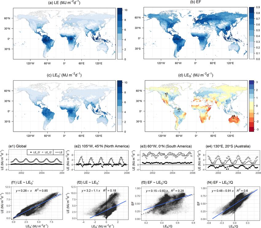
5176                   Y. Kim et al.: Relative humidity gradients as a key constraint on terrestrial water and energy fluxes

lett et al., 2014; Byrne and O’Gorman, 2018), but land–               this “high VPD leads to high LE” interpretation cannot be
atmosphere feedback processes shaping the near-surface at-            generalized because rs increases with VPD due to stomatal
mospheric state are still not well understood. In the early           closure by vegetation under high-VPD conditions (Tan et al.,
1960s, Bouchet (1963) hypothesized that land surface dry-             1978; Novick et al., 2016; Massmann et al., 2019). While
ness is coupled to the atmospheric state through LE, with             the PM equation is useful to explore biological control of LE
the Bouchet hypothesis now widely accepted (Ramírez et al.,           through rs (Jarvis and McNaughton, 1986; Peng et al., 2019),
2005; Fisher et al., 2008; Mallick et al., 2014). However, the        physical mechanisms corresponding to each term in Eq. (1)
underlying physical mechanisms for this land–atmosphere               are less intuitive due to the sensitivity of rs to VPD. As a re-
coupling still remain elusive (McNaughton and Spriggs,                sult, how the atmospheric state affects evaporation and vice
1989). Recently, McColl et al. (2019) introduced a novel              versa remains ambiguous in the PM equation.
theoretical perspective on land–atmosphere coupling which                 Is there a way to mathematically express the physical
is referred to as “surface flux equilibrium (SFE)”. They hy-          mechanisms of LE without requiring rs ? In this paper, we
pothesized that relative humidity (RH) reaches a steady-state         present a pair of equations expressing actual LE as a combi-
value in an idealized atmospheric boundary layer at daily to          nation of diabatic and adiabatic processes without requiring
monthly timescales. Under steady RH conditions (i.e., the             rs . Similar to the PM equation, our new equations are de-
SFE state), LE can be determined using only the atmospheric           rived by combining the energy balance equation with the flux
state and radiative energy. Although this method performed            gradient equations, but crucially ours do not include rs . The
well compared to actual LE observations for inland conti-             novel equations are applied empirically to eddy-covariance
nental sites (McColl and Rigden, 2020; Chen et al., 2021), a          observation sites and a global LE dataset to explore land–
further investigation is needed to understand how dynamics            atmosphere coupling processes at various spatiotemporal
of turbulent heat fluxes in the atmospheric surface layer at          scales. To do this, we decomposed observed LE into adia-
sub-daily timescales evolve to the SFE state.                         batic and diabatic components and discuss how these patterns
   A traditional way to express the atmospheric surface layer         can help to understand land–atmosphere interactions and po-
processes is to partition LE into diabatic and adiabatic pro-         tential responses under future climatic conditions.
cesses using the Penman–Monteith (PM) equation (Mon-
teith, 1965), as proposed by Monteith (1981). The PM
equation combines the energy balance equation with mass-              2     Theory
transfer theory for water vapour and sensible heat, resulting
in diabatic (radiative energy-related) and adiabatic (vapour          2.1    A pair of evaporation equations for an unsaturated
pressure deficit-related) processes for a parcel of air in con-              surface
tact with a saturated surface (Monteith, 1981).
             S                       ρcp        e∗ (Ta ) − ea         In this section, we derive a pair of evaporation equations for
LE =                  ·Q+                 ·               , (1)   an unsaturated surface. In this derivation, we assume a hor-
       S + γ rar+rs
                                S + γ rar+rs         ra
                a                        a                            izontally homogenous landscape where the sources of water
       |     {z             }   |            {z             }         vapour and heat are identical. Under this idealized condition,
         Diabatic process              Adiabatic process
                                                                      aerodynamic resistances (ra ) to heat and water vapour trans-
where S is the linearized slope of saturation vapour pressure         fers are identical. Here, ra is a parameterization of turbulent
versus temperature (hPa K−1 ), γ is the psychrometric con-            mixing due to mechanical turbulence and buoyancy driven
stant (hPa K−1 ), ρ is the air density (kg m−3 ), cp is the spe-      by surface heating.
cific heat capacity of air at constant pressure (MJ kg−1 K−1 ),           We first express LE using a flux gradient equation as LE =
                                                                      ρcp es −ea
and Q is available radiative energy (i.e., the difference be-           γ    ra , where es is the surface vapour pressure. Here,
tween net radiation (Rn ) and soil heat flux (G) expressed            the subscript s indicates the land surface which is defined
in units of W m−2 ). e∗ (Ta ) is the saturation vapour pressure       as an idealized plane specified as the sum of displacement
(hPa) corresponding to the air temperature (Ta ) measured             height and roughness length for heat (Knauer et al., 2018a;
at a reference height (typically 2 m or eddy flux measure-            Novick and Katul, 2020). If the land surface is saturated, es
ment height), and ea is vapour pressure (hPa) at the reference        becomes equivalent to the saturation vapour pressure (i.e.,
height. e∗ (Ta ) − ea is known as atmospheric vapour pressure         es = e∗ (Ts )). For an unsaturated land surface, however, rela-
deficit (VPD, expressed in units of hPa). ra is aerodynamic           tive humidity should be introduced as es = RHs e∗ (Ts ), where
resistance to heat and water vapour transfer (s m−1 ), and rs         RHs is surface relative humidity, i.e., the ratio of es to e∗ (Ts ).
is surface resistance to water vapour transfer (s m−1 ) repre-        For a vegetated surface, RHs as defined in this study rep-
senting drying soil and/or plant stomatal closure.                    resents relative humidity of the foliage surface and is con-
   In principle, high Q and VPD at the reference height in-           ceptually equivalent to surface water availability in Li and
crease the diabatic and the adiabatic terms respectively in the       Wang (2019). For a bare soil land surface, RHs represents
PM equation, and as such, Q and VPD are the two primary               soil surface relative humidity, which can be found using the
drivers of evaporation (Monteith and Unsworth, 2013). Yet,            “alpha” method that is parameterized using soil moisture

Hydrol. Earth Syst. Sci., 25, 5175–5191, 2021                                           https://doi.org/10.5194/hess-25-5175-2021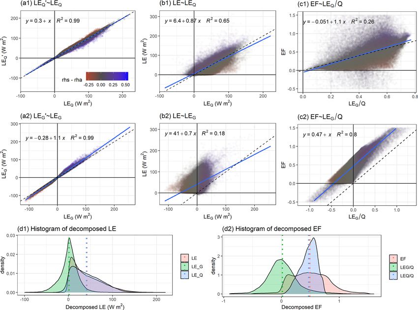
Y. Kim et al.: Relative humidity gradients as a key constraint on terrestrial water and energy fluxes                          5177

content or soil water potential (Lee and Pielke, 1992; Wu et        fundamental mechanisms of LE, particularly when it is de-
al., 2000; Cuxart and Boone,
                          ∗
                                   2020). Using RHs , LE can be     composed into its diabatic component (LEQ or LE0Q ) and its
                 ρc
written as LE = γ p RHs e r(Ta s )−ea for an unsaturated surface    adiabatic component (LEG or LE0G ). In the following sec-
condition.                                                          tions, we will discuss theoretical meanings of Eqs. (4) and
   In order to decompose LE into two individual fluxes re-          (5) in depth.
lated to temperature and relative humidity gradients, we add
−RHs e∗ (Ta ) + RHs e∗ (Ta ) (or −RHa e∗ (Ts ) + RHa e∗ (Ts )) to   2.2    Generalized Penman equation
the numerator of the flux gradient equation and rewrite LE as
follows.                                                            Before discussing PMRH in depth, we revisit the Penman
                                                                    equation (Penman, 1948) to help with the physical reason-
     ρcp     e∗ (Ts ) − e∗ (Ta )                                    ing behind our proposed framework. The widely recognized
LE =     RHs
      γ               ra                                            form of the Penman equation, which was developed as an LE
     ρcp ∗       RHs − RHa                                          model for a saturated surface, is as follows:
   +     e (Ta )                                             (2)
      γ               ra                                                                  ρcp e∗ (Ta ) ea

                                                                              S
     ρcp     e∗ (Ts ) − e∗ (Ta )                                    LE =          ·Q +                    .              (6)
LE =     RHa                                                               S +γ               S + γ ra
      γ               ra                                                   | {z }        |       {z       }
                                                                           Diabatic process   Adiabatic process
     ρcp ∗       RHs − RHa
   +     e (Ts )                                             (3)
      γ               ra                                            We rearrange this formulation to derive Eq. (7) by factor-
                                                                    ing out e∗ (Ta ) and introducing RHa = e∗e(Ta a ) into the second
We then approximate e∗ (Ts ) − e∗ (Ta ) = S(Ts − Ta ) using the     term.
saturation vapour pressure slope at the air temperature (S),
and we introduce a flux gradient equation for sensible heat                   S       ρcp e∗ (Ta ) 1 − RHa
                                                                    LE =         ·Q +             ·                              (7)
flux (i.e., H = ρcp Ts −T a
                       ra ) into Eqs. (2) and (3). Then, the
                                                                            S +γ
                                                                            | {z }    |
                                                                                        S +γ
                                                                                                {z
                                                                                                      ra
                                                                                                         }
energy balance equation is combined to substitute H with                   Diabatic process      Adiabatic process
Q − LE. As results, LE can be expressed as follows:
                                                                    Equations (6) and (7) are mathematically equivalent, but their
       RHs S       ρcp e∗ (Ta ) RHs − RHa                           interpretations are quite different. In Eq. (6), the adiabatic
LE =          ·Q +             ·          ,
     RH S + γ      RH S + γ         ra                              process is controlled by VPD at the reference height. How-
     | s {z    }   | s         {z       }                           ever, in Eq. (7), the adiabatic process acts over the verti-
       Diabatic process: LEQ    Adiabatic process: LEG
                                                                    cal RH gradient, i.e., the difference in RH from the sur-
   = LEQ + LEG                                               (4)    face to the reference height (RHa ). Since the Penman equa-
        RHa S       ρcp e∗ (Ts ) RHs − RHa                          tion is a model for saturated surfaces, 1 − RHa in Eq. (7)
LE =           ·Q +             ·                                   indicates the difference in RH over the vertical distance
      RH S + γ      RH S + γ         ra
      | a {z    }   | a         {z       }                          between the ground surface and the reference height. Ar-
       Diabatic process: LE0Q   Adiabatic process: LE0G             guably, Eq. (7) is more thermodynamically sound compared
   = LE0Q + LEG
              0
                ,                                            (5)    to Eq. (6) since RH is an ideal-gas approximation to the wa-
                                                                    ter activity (Lovell-Smith et al., 2015) which represents the
where LEQ (and LE0Q ) is a diabatic component, and LEG              chemical potential of water (µw ) (Monteith and Unsworth,
(and LE0G ) is an adiabatic component of latent heat flux.          2013; Kleidon and Schymanski, 2008). When the vertical
While the diabatic component is mainly determined by avail-         gradient of RH dissipates owing to well-developed turbu-
able energy (Q), the adiabatic component is driven by tur-          lence, the land surface and the atmosphere are in thermody-
bulent mixing and vertical gradient of RH. Monteith (1981)          namic equilibrium (Kleidon et al., 2009). Therefore, taking
originally suggested an equation equivalent to Eq. (4) for          Eq. (7) instead of Eq. (6) allows us to view the adiabatic pro-
the case when the surface does not reach saturation. To our         cess of the Penman model as an equilibration process driving
knowledge, Eq. (5) is derived for the first time here. Equa-        land–atmosphere equilibrium by bringing the surface µw to
tions (4) and (5) include RHs to compensate for eliminating         that of the atmosphere.
rs from the original PM equation.                                      As with our interpretation of the Penman model, we can
   Since the adiabatic processes in Eqs. (4) and (5) are con-       view Eqs. (4) and (5) as a generalized form of the Penman
trolled by the vertical difference of RH, we refer to Eqs. (4)      model. Here, the LEG (or LE0G ) term is an equilibration pro-
and (5) as the proposed PMRH model (Penman–Monteith                 cess between the land and the atmosphere when the land
equation expressed using RH) to distinguish it from the orig-       surface is not saturated. It is worth noting that LEG can be
inal PM model. The two Eqs. (4) and (5) are complementary           negative when RHs is less than RHa . Thus, the LEG term
to each other in that they represent distinct thermodynamic         operated by turbulent mixing acts to reduce the vertical RH
paths, each of which will be discussed in the next section.         gradient. This physical interpretation is consistent with re-
Arguably, applying PMRH can provide new insights into the           cent findings that the variance of the RH gradient tends to be

https://doi.org/10.5194/hess-25-5175-2021                                          Hydrol. Earth Syst. Sci., 25, 5175–5191, 2021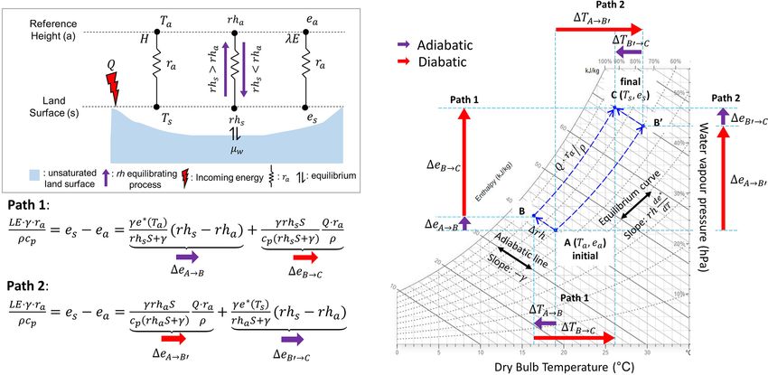
5178                 Y. Kim et al.: Relative humidity gradients as a key constraint on terrestrial water and energy fluxes

minimized over the course of the day, implying that the dif-       the adiabatic process is followed at temperature of TS (i.e.,
ference between RHs and RHa is reduced (Salvucci and Gen-          LE0G ). Path 2 is described by Eq. (5).
tine, 2013; Rigden and Salvucci, 2015). The diabatic LEQ              Therefore, one can interpret the two forms of PMRH in
(or LE0Q ) term can be understood as equilibrium LE for an         Eqs. (4) and (5) as two thermodynamic paths where the dia-
unsaturated surface, which we discuss later in Sect. 2.4.          batic and adiabatic processes occur simultaneously. It should
                                                                   be noted that the diabatic and adiabatic processes in PMRH
                                                                   are “path” functions and thus they vary by path. For instance,
2.3    Thermodynamic paths
                                                                   LEQ is slightly higher than LE0Q when RHs > RHa . Also,
                                                                   the absolute magnitude of LE0G is always bigger than that of
How can we interpret the two formulas of PMRH in Eqs. (4)          LEG when Q > 0 (i.e., vector B 0 → C is longer than vector
and (5)? To explain the two forms, the psychrometric rela-         A → B in Fig. 1).
tionship is applied to a parcel of air near an unsaturated land
surface that is under constant pressure and steadily receiving     2.4    Equilibrium LE for an unsaturated surface
radiation energy. The psychrometric diagram in Fig. 1 de-
scribes the magnitude of turbulent flux (where the length of       Another distinct characteristic of the PMRH model is the way
the arrow corresponds to the magnitude) from the view point        it defines equilibrium at the land–atmosphere interface. Un-
of a parcel of air located at a reference height (an approach      like many previous studies which focused on the steady state
based on work by Monteith, 1981). Since the parcel of air re-      of VPD (McNaughton and Jarvis, 1983; Priestley and Tay-
ceives heat and water vapour from the land surface, the final      lor, 1972; Raupach, 2001), land–atmosphere equilibrium is
state is represented by the surface condition, while the ini-      achieved in the PMRH model when the vertical RH gradient
tial state is represented by the atmospheric conditions at the     (i.e., the µw gradient) dissipates. That is, if RHs ≈ RHa , then
reference height. Therefore, the initial thermodynamic state       it follows that LEG (or LE0G ) is zero and thus LE becomes
of the air parcel can be represented by its temperature and
                                                                           RHa S
water vapour pressure such as point A in Fig. 1. The initial       LE ≈             Q.                                         (8)
state is changed by two processes as follows: (1) equilibrat-             RHa S + γ
ing between the land surface (RHs ) and the air parcel (RHa )      We note that Eq. (8) is identical to the SFE theory recently
and (2) increasing enthalpy forced by the incoming energy.         introduced by McColl et al. (2019). They hypothesized that
It should be noted that the changing process (i.e., thermody-      in many continental regions, the near-surface atmosphere is
namic path) from the initial to the final states in this discus-   in a state of equilibrium, where RH is steady with time in
sion should be understood as the magnitude of the turbulent        an idealized atmospheric boundary layer at longer than daily
heat fluxes.                                                       timescales. Equation (8) successfully predicted observed LE
   In the RH equilibrating process, the air parcel is adia-        at daily and monthly timescales for inland regions (McColl
batically cooled (or heated when RHs < RHa ) due to turbu-         and Rigden, 2020; Chen et al., 2021), which implies the
lent mixing, while the enthalpy of the parcel is not changed.      vertical RH gradient tends to evolve toward zero at longer
Therefore, the increase (decrease) in latent heat content in the   timescales than the sub-daily scale. This is logical in that
parcel is exactly balanced by a decrease (increase) in sensi-      LEG itself diminishes the vertical RH gradient over the
ble heat (A → B in Fig. 1: trajectory along constant enthalpy      course of a day.
line). This process is equivalent to the LEG term in Eq. (4).         From a different standpoint, if an observed LE is bigger or
Now, the air parcel is in thermodynamic equilibrium with           smaller than Eq. (8) at a longer timescale such as monthly,
the land surface (point B in Fig. 1). Then, the air parcel re-     it may indicate that the land surface conditions are not com-
ceives energy while the equilibrium is sustained (i.e., RHs is     pletely embedded in the near-surface atmospheric state due
steady), which increases both the temperature and absolute         to highly wet or dry land conditions. Therefore, LEG (or
water vapour content of the air parcel (B → C in Fig. 1). This     LE0G ) value and sign at monthly timescales could be a useful
process can be expressed as LEQ of Eq. (4). Consequently,          indicator reflecting land surface dryness relative to the atmo-
the thermodynamic state of the air parcel approaches point C       sphere.
in Fig. 1.                                                            When both land surface and atmosphere are saturated (i.e.,
   However, we should recognize that temperature and               RHs ≈ RHa ≈ 1), Eq. (8) becomes classical equilibrium LE
vapour pressure are “state” variables, meaning that they do                      S
                                                                   (i.e., LE ≈ S+γ  Q). This is consistent with one of the clas-
not depend on the thermodynamic path by which the system           sical definitions of equilibrium LE that defines equilibrium
arrived at its final state (Iribarne and Godson, 1981). In the     LE as evaporation from a saturated surface into saturated air
above example, we conceptually followed the adiabatic pro-         (Schmidt, 1915; Eichinger et al., 1996; Raupach, 2001; Mc-
cess first and then the diabatic process (Path 1 in Fig. 1), but   Coll, 2020). Therefore, we can regard Eq. (8) as a generalized
one can imagine the opposite order. If we choose Path 2 in         equilibrium LE for an unsaturated surface.
Fig. 1, the diabatic process comes first, and thus RHa instead
of RHs is preserved while enthalpy increases (i.e., LE0Q ), and

Hydrol. Earth Syst. Sci., 25, 5175–5191, 2021                                       https://doi.org/10.5194/hess-25-5175-2021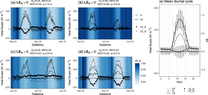
Y. Kim et al.: Relative humidity gradients as a key constraint on terrestrial water and energy fluxes                                   5179

Figure 1. Schematic conceptualization of the PMRH model and psychrometric relationship of PMRH . The example psychrometric chart is
                                                                 ρc                                               ρc
modified from Marsh (2018). Path 1 represents Eq. (4) divided by γ rpa while Path 2 represents Eq. (5) divided by γ rpa . Here, the enthalpy
change of the air parcel is defined as Q·ra       −1
                                        ρ (kJ kg ). It should be noted that the difference between the initial and the final states represents
the magnitude of the turbulent heat fluxes instead of changes in atmospheric state.

3     Materials and methods                                              sons via furrow irrigation events, except for 2016 when there
                                                                         was no irrigation due to crop replanting. Due to the ratoon-
In the following sections, we present a novel physical de-               ing practice (i.e., sugarcane cutting each year followed by
composition of LE from PMRH into LEQ and LEG compo-                      resprouting without replanting, detailed explanation in the
nents to aid in understanding the governing physics of LE.               Supplement), the sugarcane growing seasons varied by year,
Also, the proportion of net available energy consumed in                 which provided an opportunity to explore distinct and varied
evapotranspiration,
                   known as the evaporative fraction (EF)              combinations of land surface vs. atmospheric aridity condi-
                                 LE
  EF = Q is decomposed into QQ and LEQG . We conducted
        LE                                                               tions.
a detailed diagnostic analysis of the PMRH model using the                  The measured LE and sensible heat flux (H ) were qual-
multi-year record of an eddy covariance (EC) flux observa-               ity controlled following Morillas et al. (2019) (details in the
tion site located in a wet–dry tropical climate. We also ap-             Supplement). For the study period, the surface energy bal-
plied the PMRH model to the 212 EC sites represented in                  ance closure (i.e., LE+H
                                                                                               Rn −G ) of 30 min data was 86 %, which is
the FLUXNET2015 dataset (Pastorello et al., 2020) and to                 typical of high-quality eddy-covariance datasets (Wilson et
the FLUXCOM global LE product (Jung et al., 2019). We                    al., 2002). When canopy height was less than 1 m, the sur-
describe the local and global datasets and analysis methods              face energy balance was almost closed (97 %), whereas the
here before presenting the results.                                      closure was 83 % when canopy height was higher than 1 m. It
                                                                         is expected that unmeasured canopy and soil heat storages in
3.1    In situ EC flux observation                                       this site are significant because the sugarcane canopy grew up
                                                                         to 3.6 m tall with a dense canopy. For instance, Meyers and
In situ half-hourly EC observations used in this study were              Hollinger (2004) showed that storage term comprised 14 %
made from 2015 to 2018 on a ratoon sugarcane farm in                     of net radiation for a maize field with a 3 m canopy height and
the province of Guanacaste, Costa Rica (10◦ 250 07.6000 N,               8 % of net radiation for a soybean field with a 0.9 m canopy
85◦ 280 22.2200 W). The site has a wet–dry tropical climate              height, implying larger heat storage capacities for taller crop
with a dry season from December to March and a median                    canopies. Also, since our study site is located within a ho-
monthly air temperature ranging from 27 to 30 ◦ C. The study             mogenous landscape (Fig. S1 in the Supplement), horizontal
site experienced a significant drought in 2015 as the lowest             and vertical advective flux divergence and the influence of
precipitation rate in Fig. 2b (Hund et al., 2018; Morillas et            secondary circulations on the energy balance closure may be
al., 2019). The site was irrigated occasionally during dry sea-

https://doi.org/10.5194/hess-25-5175-2021                                               Hydrol. Earth Syst. Sci., 25, 5175–5191, 2021
5180 Y. Kim et al.: Relative humidity gradients as a key constraint on terrestrial water and energy fluxes
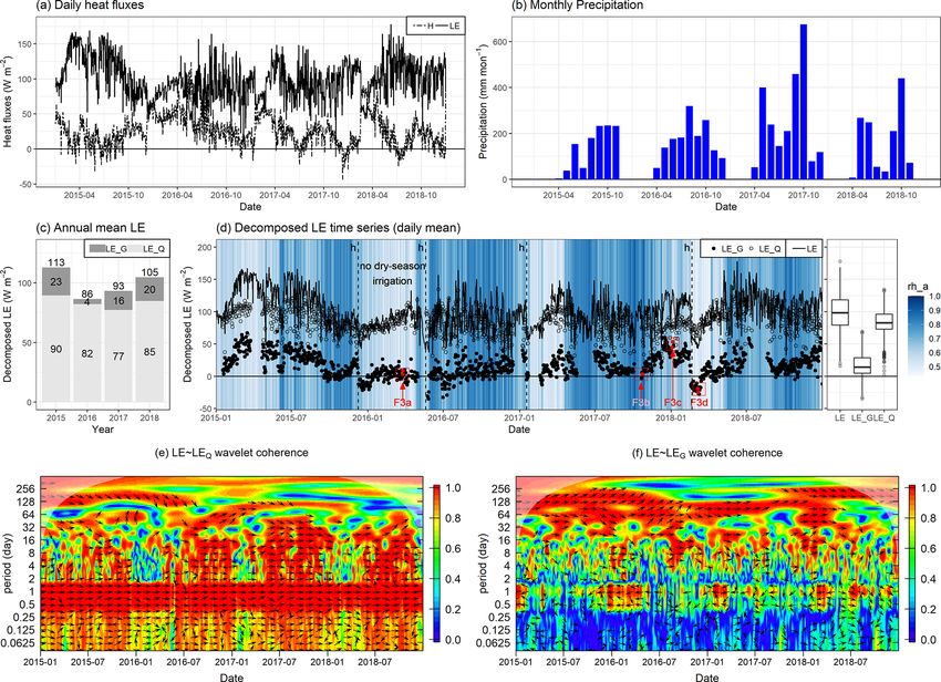
Figure 2. Time series for the sugarcane EC tower site in Costa Rica. Panel (a) is daily heat fluxes and panel (b) is monthly precipitation.
Panel (c) is mean annual LE and its two components, and (d) is time series of LE, LEQ , and LE with a background colour of RHa . Dashed
lines with “h” in panel (d) indicate sugarcane harvest. Panels (e) and (f) are wavelet coherence of LE with LEQ and LE with LEG . Red and
blue colours indicate high and low correlation, respectively. Arrows (pointing right: in-phase; left: antiphase) only appear when the coherence
is significant (p < 0.01).
marginal (Mauder et al., 2020; Leuning et al., 2012). There- The first term on the right-hand side of Eq. (9) is the aero-
fore, considering the homogenous landscape of the study site dynamic component, and the second term is the boundary
as well as a possible significant role of unmeasured canopy layer component. Here, u∗ is friction velocity, k is the von
and soil heat storages, we did not force the energy closure. Kármán constant (0.41), d is the zero-plane displacement
Consequently, we defined Q as the sum of LE and H instead height (d = 0.7zh ), z0 m is the roughness length for momen-
of Rn − G. In doing so, we in effect attribute the cause of the tum (z0 m = 0.1zh ), and ψh is the integrated form of the sta-
surface energy imbalance to unmeasured heat storage terms bility correction function. zh is canopy height based on man-
following Moon et al. (2020). ual measurements taken during regular maintenance visits.
In order to decompose LE into LEQ and LEG , we first ra was estimated using the bigleaf R package (Knauer et al.,
estimated half-hourly aerodynamic resistance (ra ) by consid- 2018a).
ering aerodynamic resistance to momentum transfer and the By rearranging Eq. (2), RHs can be calculated using
additional boundary layer resistance for heat and mass trans-
γ LEra /ρcp + ea
fer (or excess resistance) (Thom, 1972; Knauer et al., 2018a). RHs = . (10)
SH ra /ρcp + e∗ (Ta )
h i Negative H and inaccurate ra modelling sometimes yielded
zr −d
ln z0 m − ψh negative RHs or values greater than 1, especially at night-
ra = + 6.2u−0.67
∗ (9) time. In these cases, RHs was assigned the value of 1 follow-
ku∗
Hydrol. Earth Syst. Sci., 25, 5175–5191, 2021 https://doi.org/10.5194/hess-25-5175-2021Y. Kim et al.: Relative humidity gradients as a key constraint on terrestrial water and energy fluxes 5181
ing the approach described in the bigleaf R package (Knauer 3.3 FLUXCOM
et al., 2018a). We then estimated LEQ and LEG from Eq. (4).
In order to explore the timescale of the covariances for The FLUXCOM dataset (Jung et al., 2019) is a global-
LE ∼ LEQ and LE ∼ LEG in the frequency domain, we ap- scale machine learning ensemble product which upscales
plied wavelet coherence analysis using the WaveletComp R FLUXNET observations (Baldocchi et al., 2001) using Mod-
package (Roesch and Schmidbauer, 2014). The package is erate Resolution Imaging Spectroradiometer (MODIS) satel-
designed to apply the continuous wavelet transform using the lite data and reanalysis meteorological data. In this study we
Morlet wavelet, which is a popular approach to analyze hy- used the monthly LE FLUXCOM dataset (0.5◦ resolution)
drological and micrometeorological datasets (Hatala et al., modelled using MODIS and ECMWF ERA5 reanalysis data
2012; Johnson et al., 2013). A total time series of half-hourly (Hersbach et al., 2020).
decomposed LE for the 4-year measurement period was used We obtained Q and LE from the FLUXCOM output, and
to estimate localized coherence and phase angle. The wavelet air temperature and dew point temperature were retrieved
coherence can be interpreted as the local correlation between from ERA5 monthly averaged data (2 m height). RH, S, and
two variables in the frequency–time domain (where red in- γ were calculated from ERA5 data, and then LE0Q was cal-
dicates high correlation). A 0◦ phase angle (arrow pointing culated. LE0G was then estimated by subtracting LE0Q from
right) indicates periods of positive correlation, while a 180◦ LE.
phase angle (arrow pointing left) indicates periods of nega-
tive correlation.
4 Results
3.2 FLUXNET2015
4.1 Decomposition analysis of in situ EC flux
The daily-scale FLUXNET2015 dataset, which includes 212 observation
empirical eddy-covariance flux tower sites around the globe
(Pastorello et al., 2020), was used in this study. The turbulent Application results of the PMRH model to the observed LE
heat fluxes, net radiation, soil heat flux, air temperature, rel- at an irrigated sugarcane farm in Costa Rica are depicted in
ative humidity, wind speed, friction velocity, and barometric Fig. 2. The decomposition analysis of observed LE shows
pressure were obtained from the dataset. For this analysis, that while LEQ is the major component of LE, LEG variabil-
we only included daily data for periods for which the quality ity plays a non-negligible role in seasonal and interannual
control flag indicated more than 80 % half-hourly data were behaviour of LE. In terms of absolute magnitude, the LEQ
present (i.e., measured data in general, or good-quality gap- term can closely approximate LE, and LEG only represents
filled data in cases of partially missing data). 15 % of total evaporation (Fig. 2c). Also, positive coherence
In order to decompose daily LE into LEQ and LEG , we between LE and LEQ was strong over the entire period of ob-
estimated daily aerodynamic resistance (ra ) by Eq. (11) in- servation, particularly at diurnal to multiday timescales (0.5–
stead of Eq. (9) since canopy and measurement heights are 32 d), implying variability of LE is largely determined by
unknown (Thom, 1972; Knauer et al., 2018a). LEQ variability (i.e., red coloured regions in Fig. 2e).
Although absolute magnitude of LEG was much smaller
u2∗ than that of LEQ , the interannual variability of LEG was
ra = + 6.2u−0.67
∗ , (11)
u (zr ) larger than the interannual variability of LEQ (Fig. 2c). Fur-
thermore, LE and LEG also had a strong positive correlation
where u(zr ) is reference height wind speed. ra was estimated on longer timescales (32–365 d) (i.e., red coloured regions
using the bigleaf R package (Knauer et al., 2018a), and RHs in Fig. 2f). Unexpectedly, a negative correlation between LE
was calculated from Eq. (8). and LEG at the diurnal timescale was observed in the wavelet
LEQ and LE0Q were calculated using RHa and RHs follow- analysis only when the land surface was dry and there was
ing Eqs. (4) and (5), and then LEG and LE0G were calculated little vegetation (i.e., after harvest) or during a year in which
by subtracting LEQ and LE0Q from LE. To calculate LEQ there was no dry season irrigation applied. Also, we found
and LE0Q , we define Q as LE + H , but it should be noted that EF variability is mostly determined by LEG variability
that this approach can include systematic uncertainty since since the diurnal and seasonal signals of Q are removed from
the sum of LE and H measured by eddy covariance is typ- LE in EF. Interestingly, the annual mean LEG was the high-
ically lower than Rn − G (i.e., conditions referred to as the est in 2015, a drought year in which RHa and precipitation
energy balance closure problem; Wilson et al., 2002). To in- were generally lower than for the other years, while the an-
vestigate the effect of a lack of energy balance closure on nual mean LEG was close to zero in 2016 when there was no
resulting LE terms, we provide Fig. S2 that was generated application of dry season irrigation due to crop replanting.
by (1) defining Q as Rn − G and (2) correcting LE and H To explore the diurnal behaviour of decomposed LE, we
based on the assumption that the Bowen ratio (B = H /LE) selected different surficial and atmospheric conditions when
is correct (Pastorello et al., 2020). LEG was zero, positive, or negative in Fig. 3. In the 2016
https://doi.org/10.5194/hess-25-5175-2021 Hydrol. Earth Syst. Sci., 25, 5175–5191, 20215182 Y. Kim et al.: Relative humidity gradients as a key constraint on terrestrial water and energy fluxes
Figure 3. Half-hourly time series of heat fluxes and the two components indicated in Fig. 2d. The background colour represents RHs . Here,
RHa is mean atmospheric relative humidity, SM is volumetric soil water content, normalized difference vegetation index (NDVI) represents
vegetation status, and zh is canopy height. Panel (e) presents the long-term mean diurnal cycle of decomposed LE (dots) and EF (dashed
line).
dry season, LEG was close to zero as a daily average value, 4.2 Decomposition analysis of the FLUXNET2015
as a result of negative daytime and positive nighttime LEG dataset
values due to dry air and dry soil conditions (no irrigation)
and an undeveloped vegetation canopy (Fig. 3a). Daily LEG
was also close to zero during wet season conditions (e.g.,
Fig. 3b). In this case, LEG was near zero during both day- Decomposition analysis of the daily FLUXNET2015 dataset
time and nighttime periods due to near-saturated atmospheric is illustrated in Fig. 4. In terms of absolute magnitude of each
and land surface conditions. These two cases show that “dry term, the majority of LEG (and LE0G ) values ranged from
land–dry air” or “wet land–wet air” conditions can each lead −50 to 50 W m−2 , with some exceptional values approach-
to daily scale land–atmosphere equilibrium, although the di- ing ±100 W m−2 . On the other hand, LEQ (and LE0Q ) values
urnal pattern of LEG is starkly different for dry land–dry air ranged from 0 to 150 W m−2 .
vs. wet land–wet air conditions. One of the interesting findings from the decomposition
Meanwhile, when RHa was low and the canopy was well- analysis of the FLUXNET2015 dataset was that differences
developed, LEG was found to be positive during both day- between LEQ and LE0Q are marginal at a daily timescale (the
time and nighttime periods (Fig. 3c). On the other hand, dur- slope is close to 1 in Fig. 4a1). This result implies that al-
ing post-harvest conditions when vegetative canopy cover though the diabatic processes expressed by Eqs. (4) and (5)
was minimal and air and soil moisture levels were low, daily are different in magnitude due to the difference between RHs
LEG was found to be negative as a result of negative day- and RHa (see Sect. 2.3), these differences are practically neg-
time and positive nighttime LEG (Fig. 3d). Diurnal variation ligible. This is an important point since LE0Q can be deter-
in RHs was maximized when daily LEG was negative, im- mined simply and directly using reference height meteoro-
plying a large diurnal fluctuation in surface temperature un- logical measurements, while LEQ is required to know RHs .
der the drier land surface conditions. Regarding the overall As for the adiabatic terms, LE0G is roughly 1.1 times LEG
diurnal pattern, LEG generally declined during the morning at a daily timescale (Fig. 4a2), which is consistent with the
and increased in the afternoon, which is consistent with the theory regarding their respective thermodynamic paths. As
well-known diurnal pattern of EF (Gentine et al., 2011, 2007) we discussed in Sect. 2.3, the absolute magnitude of LE0G
(Fig. 3e). must be bigger than that of LEG when available energy is
positive. Therefore, the empirical relationship between LEG
and LE0G in Fig. 4a2 is a consequence of a physical principle,
and this result may provide the following empirical relation-
Hydrol. Earth Syst. Sci., 25, 5175–5191, 2021 https://doi.org/10.5194/hess-25-5175-2021Y. Kim et al.: Relative humidity gradients as a key constraint on terrestrial water and energy fluxes 5183
Figure 4. FLUXNET2015 daily-scale decomposed LE for 212 sites and 1532 site years. Panels (a1) and (a2) are linear regressions of LE0Q on
LEQ and LE0G on LEG . Panels (b1) and (b2) are linear regressions of LE on LEQ and LE on LEG . Panels (c1) and (c2) are linear regressions
of EF on LEQ /Q and EF on LEG /Q. In these panels, daily EF data within a range from −1 to 1.5 are only shown. Here, dashed lines are
one-to-one lines, blue lines are regression lines, and colour represents RHs − RHa . Panels (d1) and (d2) are histograms of decomposed LE
and EF with mean values (dotted lines). To correct for lack of energy balance closure, Q was set equal to LE + H in all calculations.
ship. stead of LEG (R 2 = 0.18) as depicted in Fig. 4b1 and b2.
Nevertheless, FLUXNET2015 data also suggest that LEG is
ρcp e∗ (Ta ) RHs − RHa ρcp e∗ (Ts ) RHs − RHa
1.1 · ≈ · the main driver of local-scale variability of EF at the daily
RHs S + γ ra RHa S + γ ra timescale (Fig. 4c1 and c2). Although the mean value of daily
e∗ (Ta ) e∗ (Ts ) LE
EF is close to the mean value of QQ , the variation in daily EF
1.1 ≈ (12)
RHs S + γ RHa S + γ
depends more on the variation in LEQG (Fig. 4d2). It should be
Equation (12) reveals an emergent daily timescale relation- noted that Figs. 4 and S2 are almost identical (Fig. S2 repeats
ship between temperature and relative humidity which has the presentation shown in Fig. 4 using the value computed
the potential to be used as a supplementary equation in fu- when forcing energy balance closure), implying that the lack
ture research. of surface energy balance closure for EC observations does
Another important finding of the decomposition analysis not significantly impact our analyses and interpretations.
is the global-scale land–atmosphere equilibrium. Our analy-
sis in Fig. 4d1 indicates that the mean value of daily LEG of 4.3 Decomposition analysis of FLUXCOM dataset
all FLUXNET2015 sites is close to zero, implying the global
mean RH gradient is near zero at a daily timescale. Impor- We then applied the PMRH model to the FLUXCOM dataset,
tantly, LE is primarily determined by LEQ (R 2 = 0.65) in- a benchmark global LE data product (Jung et al., 2019). As
https://doi.org/10.5194/hess-25-5175-2021 Hydrol. Earth Syst. Sci., 25, 5175–5191, 20215184 Y. Kim et al.: Relative humidity gradients as a key constraint on terrestrial water and energy fluxes
shown in Fig. 5a and c, the spatial patterns of the annual tion process of RH gradient at a sub-daily scale resulting in
mean LE and LE0Q were similar. For instance, both LE and a small gradient of RH on daily average.
LE0Q show the highest values around the Equator at an an- We found positive nighttime LEG values regardless of wet
nual timescale, which is mainly due to the energy available or dry conditions, except when the atmosphere was fully sat-
in this region. Also, spatial variability of LE is mostly de- urated (Fig. 3). This result is a natural consequence since the
termined by LE0Q (R 2 = 0.85 and slope = 1) rather than by land surface is close to saturation at night. This finding sug-
LE0G (R 2 = 0.18) (Fig. 5f1 and f2). This result is consistent gests that LEG is a dominant contributor to nighttime evapo-
with Eq. (8) and the SFE theory. In other words, the land ration since available energy is close to zero at night. It is im-
surface is generally under thermodynamic equilibrium with portant since nighttime evaporation is a non-negligible com-
the atmosphere at the global–annual scale (i.e., RHs ≈ RHa ). ponent of total ET (Padrón et al., 2020).
Furthermore, the monthly time series of global LE and its Unlike nighttime LEG values, the direction and the mag-
two components in Fig. 5e1 show that (i) LE0G is consistently nitude of the daytime LEG are highly dependent on the land
close to zero at the global scale and (ii) the seasonal variabil- surface dryness. For example, the U-shape diurnal cycles of
ity of global LE is primarily determined by LE0Q . LEG are apparent only when the land surface is dry, which
However, while mean annual LE0G was close to zero in is confirmed by the negative wavelet coherence between LE
broad areas (particularly in high-latitude regions) as exem- and LEG at the diurnal timescale in Fig. 2f. When the land
plified in Fig. 5e2, it was distinctly positive or negative at the surface is wetter than the atmosphere, LEG values were posi-
annual scale for many regions (Fig. 5d). In humid tropical re- tive even in the daytime, and thus the U-shape diurnal cycles
gions like the Amazon basin where moisture convergence is of LEG did not appear (Fig. 3c). The positive LEG during
large, LE0G was generally positive, whereas arid regions such daytime periods may be explained as a consequence of warm
as Australia were characterized by negative LE0G (Fig. 5e3 and dry air entrainment at the top of the atmospheric bound-
and e4). Here, positive LE0G (i.e., RHs > RHa ) indicates the ary layer and/or horizontal advection of sensible heat which
land surface is wetter than the near-surface atmosphere while may reduce atmospheric relative humidity (Baldocchi et al.,
negative LE0G (i.e., RHs < RHa ) implies a drier land surface 2016; de Bruin et al., 2016). Indeed, a strong entrainment
than the atmosphere. Therefore, the sign of LE0G in Fig. 5d effect and/or local advection of sensible heat are common
can be interpreted as representing land surface dryness rela- phenomena for irrigated agriculture (Baldocchi et al., 2016;
tive to the atmosphere at an annual timescale. de Bruin and Trigo, 2019), and the irrigated sugarcane site
The spatial pattern of LE0G is similar to the spatial pattern shows that the annual mean LEG was always positive except
of EF, but differs from the spatial pattern of LE0Q (Fig. 5b). for in 2016 when there was no application of dry season irri-
For example, EF was high in not only tropical regions but gation.
also temperate climates such as Mediterranean regions, and
this spatial pattern is well matched with the spatial pattern 5.2 LEG at daily to annual timescales
of LE0G but not LE0Q . The finding that the spatial variation in
EF is primarily controlled by LE0G instead of LE0Q was sup- As described in the theory section, land–atmosphere equi-
ported by correlation analyses in Fig. 5f3 and f4 (R 2 = 0.60 librium is achieved when LEG approaches zero and thus
LE0 LE0 LE reduces to Eq. (8) at a timescale longer than sub-
for EF ∼ QG and R 2 = 0.28 for EF ∼ QQ ). This is under- daily. The decomposed terms derived from both the empir-
standable in that EF is a reflection of the land surface dry- ical FLUXNET2015 and model-based FLUXCOM datasets
ness (Gentine et al., 2011), and LE0G reveals the land surface show that the global mean for LEG is near zero, implying
dryness relative to the atmosphere. global-scale land–atmosphere equilibrium (Figs. 4 and 5).
This result extends the SFE theory of McColl et al. (2019).
5 Discussion Although LEG is not always near zero for timescales longer
than sub-daily, moisture convergence and divergence at
5.1 LEG at sub-daily scale the global scale tend to balance each other out, result-
ing in global-scale land–atmosphere equilibrium on longer
Salvucci and Gentine (2013) found that the variance of the timescales (Fig. 5e1).
RH gradient tends to be minimized over the course of the From a different perspective, non-zero LEG value and its
day. Based on this empirical finding, they developed an ap- sign (+ vs. −) at the local scale can be understood as an
proach to predict LE only using standard meteorological indicator reflecting land surface dryness relative to the at-
measurements, and this approach accurately predicted actual mosphere. We found that LEG clearly distinguishes spatially
LE (Rigden and Salvucci, 2015, 2017). Our PMRH model wet and dry regions around the world (Fig. 5 d). We also
provides theoretical support for their approach in that LEG found that the spatiotemporal variability of EF was largely
acts to reduce the RH gradient. Indeed, the U-shape diurnal explained by LEG instead of LEQ (Figs. 4c2 and 5f4). These
cycles of LEG in Fig. 3 (positive nighttime and negative day- results demonstrate the usefulness of LEG to quantify land
time) show the direction and the magnitude of the equilibra- surface dryness. Some previous studies introduced evapora-
Hydrol. Earth Syst. Sci., 25, 5175–5191, 2021 https://doi.org/10.5194/hess-25-5175-2021Y. Kim et al.: Relative humidity gradients as a key constraint on terrestrial water and energy fluxes 5185
Figure 5. Mean annual LE, EF, LE0Q , and LE0G from 2001 to 2005 (panels a, b, c, and d, respectively). Panel (e1) is a time series of monthly
global average LE and the two components LE0G and LE0Q . Panels (e2), (e3), and (e4) are time series at specific locations highlighted in
panel (d). Panels (f1), (f2), (f3), and (f4) are spatial linear regressions of LE on LE0Q , LE on LE0G , EF on LE0Q /Q, and EF on LE0G /Q,
respectively.
tive stress index or evaporation deficit index based on the 5.3 Future applications
ratio (or difference) between potential evaporation and ac-
tual evaporation (Anderson et al., 2015; Kim and Rhee, 2016;
Fisher et al., 2020; Baldocchi et al., 2021), but these meth- In this study, we present the PMRH model and demonstrate
ods are highly dependent on the way one calculates potential its utility for exploratory and diagnostic purposes. However,
evaporation. Unlike potential evaporation (which is a theo- the model has potential applications for other purposes. One
retical value), LEG is a true physical quantity, and negative possible application is to use PMRH to predict actual ET.
LEG values directly reflect water-limited land surface con- Although the original PM equation is widely used to pre-
ditions. Therefore, we suggest applying our decomposition dict evapotranspiration (e.g., Leuning et al., 2008; Mu et
method to better quantify evaporative stress. al., 2011; Mallick et al., 2014), its accuracy often relies on
parameterized surface resistance models (Polhamus et al.,
2013). Since our PMRH formulation does not include surface
https://doi.org/10.5194/hess-25-5175-2021 Hydrol. Earth Syst. Sci., 25, 5175–5191, 20215186 Y. Kim et al.: Relative humidity gradients as a key constraint on terrestrial water and energy fluxes
resistance, it could represent a good alternative. As shown in could cause a systematic uncertainty in estimating rs when
the results section, LE0Q can be calculated using typical mete- using the PM equation (Knauer et al., 2018b; Wohlfahrt et
orological data without additional surface parameters. Also, al., 2009), and this issue may affect the diagnostic analyses
we found that LE0Q alone can be used effectively to approx- using the PMRH . In this study, we did not force the energy
imate LE. If the remotely sensed land surface conditions are balance closure and attributed the cause of observed sur-
known (e.g., soil moisture and/or land surface temperature), face energy imbalances to unmeasured heat storage terms
actual LE may be more accurately predicted by incorporat- for the Costa Rica EC site due to the possibly significant
ing the LEG term. To estimate the LEG term, RHs may be role of the heat storage term (details in the Sect. 3.1). Wehr
estimated based on soil moisture and/or land surface temper- and Saleska (2021) recently demonstrated that regardless of
ature data. For example, Eq. (12), which is well supported by whether the lack of energy balance closure of EC observa-
observations (Fig. 4a2) and on a physical basis, may be used tions is due to LE + H or is due to Rn − G, applying the
to calculate RHs . flux gradient equation to observed LE and H without energy
Another possible application is to study impacts of cli- balance correction is the best way to determine rs . This is be-
mate change and land use and land cover change on sur- cause applying the flux gradient equation to observed LE and
face energy partitioning and evaporation. Changes in the at- H can dispense with the unnecessary assumption of energy
mospheric state such as temperature and relative humidity, balance closure. They showed that bias introduced by under-
as well as changes in the land surface characteristics such estimated LE and H is smaller than the bias introduced by
as albedo and aerodynamic roughness, can alter evaporation the energy balance closure assumption. This finding may be
(Lee et al., 2011; Wang et al., 2018). However, how these applied to our analysis in calculating RHs instead of rs .
changes affect terrestrial energy partitioning and ET is still As for the FLUXNET2015 dataset, we provide an al-
unclear. Indeed, there is a large discrepancy in long-term LE ternate analysis using energy-balance-corrected LE and H
trends among current land surface models (Pan et al., 2020). (Bowen ratio preserving method in Pastorello et al., 2020)
Since PMRH makes it possible to physically decompose LE in the Supplement. We found that the results for corrected
into adiabatic and diabatic thermodynamic components, the and uncorrected versions were almost identical, which can
PMRH approach can be useful to understand how environ- be viewed as a natural consequence since in Eq. (10) LE and
mental changes affect surface energy partitioning. For in- H are included in the numerator and denominator respec-
stance, trend analysis for the decomposed LE using PMRH tively. Multiplying the same ratio to LE and H in Eq. (10) to
could contribute to improve our understanding of earth’s cli- correct LE and H based on the Bowen ratio method does not
mate system and water cycle. significantly change the resulting RHs . Therefore, the lack of
surface energy balance closure does not significantly impact
5.4 Potential caveats our analyses and interpretations unless the lack of energy bal-
ance is dominated by LE only or H only. If the lack of energy
Despite the insights it can offer, the PMRH model shares sev- balance is dominated by LE only or H only, our results and
eral limitations with the traditional PM model. First, PM- interpretation may include systematic bias.
style equations linearize the exponential relationship be- Finally, there are several ways to calculate aerodynamic
tween saturation vapour pressure and temperature (Clausius– resistance, and the chosen form for ra may affect the re-
Clapeyron relation), but the linearization can cause bias when sults. However, the influence of this choice is expected to be
the temperature difference between surface and atmosphere marginal compared to the energy balance problem. Knauer
is substantial (Paw U and Gao, 1988; McColl, 2020). Sec- et al. (2018b) showed that uncertainty caused by different ra
ond, the PMRH model assumes that aerodynamic resistance values on surface conductance is low compared to the energy
for heat and water vapour is identical, which implicitly relies balance closure problem. This finding can be applied to our
on the assumption that the ratio of the turbulent Schmidt to analysis. Specifically, in Eq. (10), ra is multiplied by both
Prandtl numbers is unity (Knauer et al., 2018a). This similar- denominator and numerator, and thus a small difference in ra
ity assumption cannot be held in some cases, especially when should not significantly affect the resulting RHs .
advective flux divergence is significant (Lee et al., 2004). The
third potential caveat is that we define the land surface as
an idealized single plane that is equivalent to the “bigleaf” 6 Conclusions
representation of the traditional PM equation, but this ap-
proach ignores profiles of temperature and humidity inside We have shown that our novel PMRH model provides a new
the canopy (Bonan et al., 2021). opportunity to understand the governing physics of the ter-
Another potential caveat concerns the surface energy bal- restrial energy budget. Specifically, the PMRH model helps
ance. The surface energy balance is a governing equation of to illustrate how the land surface conditions become encoded
the PM-style models, but it is not satisfied in typical EC ob- to the atmospheric state by partitioning LE into two ther-
servations, which is referred to as the “surface energy balance modynamic processes. “Dry land–dry air” or “wet land–wet
closure problem” (Wilson et al., 2002). This closure problem air” conditions can each lead to daily scale land–atmosphere
Hydrol. Earth Syst. Sci., 25, 5175–5191, 2021 https://doi.org/10.5194/hess-25-5175-2021Y. Kim et al.: Relative humidity gradients as a key constraint on terrestrial water and energy fluxes 5187
equilibrium, although the diurnal pattern of the equilibration Financial support. This research has been supported by the Joint
process (i.e., LEG ) is starkly different. Our findings sug- Programming Initiative Water challenges for a changing world
gest that while LEG is a primary component determining (Agricultural Water Innovations in the Tropics).
EF, spatiotemporal variability of LEQ alone can adequately
represent the variability of LE. We found global-scale land–
atmosphere equilibrium at daily to annual scales, which im- Review statement. This paper was edited by Anke Hildebrandt and
plies that global LE can be simply determined by the atmo- reviewed by two anonymous referees.
spheric state and radiative energy without any surface con-
straint required to represent spatial heterogeneity and physio-
logical influences. From a different perspective, the non-zero
LEG value at a local scale can be understood as an indicator References
revealing land surface dryness. Questions remain regarding
how LEQ and LEG will be influenced in relation to changing Ameriflux: CR-Fsc site (Filadelfia sugar cane cropland), available
climatic and land surface conditions and how these changes at: https://ameriflux.lbl.gov/, last access: 22 September 2021.
might affect the climate system at differing spatial and tem- Anderson, M. C., Zolin, C. A., Hain, C. R., Semmens, K., Tugrul
Yilmaz, M., and Gao, F.: Comparison of satellite-derived LAI
poral scales through positive or negative feedbacks.
and precipitation anomalies over Brazil with a thermal infrared-
based Evaporative Stress Index for 2003–2013, J. Hydrol., 526,
287–302, https://doi.org/10.1016/j.jhydrol.2015.01.005, 2015.
Data availability. The FLUXNET2015 dataset is available in https: Baldocchi, D., Falge, E., Gu, L., Olson, R., Hollinger, D.,
//fluxnet.org/data/download-data/ (FLUXET community, 2019). Running, S., Anthoni, P., Bernhofer, C., Davis, K., and
The highlighted sugarcane eddy covariance site dataset will be Evans, R.: FLUXNET: A new tool to study the tempo-
available in AmeriFlux (by December 2021, https://ameriflux.lbl. ral and spatial variability of ecosystem-scale carbon diox-
gov/, AmeriFlux, 2021). The FLUXCOM dataset is available in ide, water vapor, and energy flux densities, B. Am. Me-
http://www.fluxcom.org/EF-Download/ (FLUXCOM, 2021). teorol. Soc., 82, 2415–2434, https://doi.org/10.1175/1520-
0477(2001)0822.3.CO;2, 2001.
Baldocchi, D., Knox, S., Dronova, I., Verfaillie, J., Oikawa,
Supplement. The supplement related to this article is available on- P., Sturtevant, C., Matthes, J. H., and Detto, M.: The
line at: https://doi.org/10.5194/hess-25-5175-2021-supplement. impact of expanding flooded land area on the annual
evaporation of rice, Agr. Forest Meteorol., 223, 181–193,
https://doi.org/10.1016/j.agrformet.2016.04.001, 2016.
Author contributions. YK and MSJ designed research; UW pro- Baldocchi, D., Ma, S., and Verfaillie, J.: On the inter- and intra-
vided FLUXCOM data; YK, LM, and MSJ performed research; YK annual variability of ecosystem evapotranspiration and water use
analyzed data; YK, MG, TAB, LM, and MSJ wrote the paper. efficiency of an oak savanna and annual grassland subjected to
booms and busts in rainfall, Glob. Change Biol., 27, 359–375,
https://doi.org/10.1111/gcb.15414, 2021.
Competing interests. The authors declare that they have no conflict Bonan, G. B., Patton, E. G., Finnigan, J. J., Baldocchi, D. D., and
of interest. Harman, I. N.: Moving beyond the incorrect but useful paradigm:
reevaluating big-leaf and multilayer plant canopies to model
biosphere-atmosphere fluxes – a review, Agr. Forest Meteorol.,
Disclaimer. Publisher’s note: Copernicus Publications remains 306, 108435, https://doi.org/10.1016/j.agrformet.2021.108435,
neutral with regard to jurisdictional claims in published maps and 2021.
institutional affiliations. Bouchet, R. J.: Evapotranspiration réelle et potentielle, signification
climatique, IAHS Publ, 62, 134–142, 1963.
Byrne, M. P. and O’Gorman, P. A.: Understanding Decreases
in Land Relative Humidity with Global Warming: Concep-
Acknowledgements. We want to thank Iain Hawthorne, Pável
tual Model and GCM Simulations, J. Climate, 29, 9045–9061,
Bautista, Silja Hund, Cameron Webster, Gretel Rojas Hernandez,
https://doi.org/10.1175/jcli-d-16-0351.1, 2016.
Guillermo Duran Sanabria, Andrea Suarez Serrano, Ana Maria Du-
Byrne, M. P. and O’Gorman, P. A.: Trends in continen-
ran, Martin Martinez, and Fermín Subirós Ruiz for field and logis-
tal temperature and humidity directly linked to ocean
tical support. We also thank Martin Jung, the principal investigator
warming, P. Natl. Acad. Sci. USA, 115, 4863–4868,
of the FLUXCOM dataset. The authors would like to thank the EU
https://doi.org/10.1073/pnas.1722312115, 2018.
and NSERC for funding, in the frame of the collaborative inter-
Chen, S., McColl, K. A., Berg, A., and Huang, Y.: Surface flux equi-
national Consortium AgWIT financed under the ERA-NET Water-
librium estimates of evapotranspiration at large spatial scales, J.
Works2015 Cofunded Call. This ERA-NET is an integral part of
Hydrometeorol., 22, 765–779, https://doi.org/10.1175/jhm-d-20-
the 2016 Joint Activities developed by the Water Challenges for a
0204.1, 2021.
Changing World Joint Programme Initiative (Water JPI).
Cuxart, J. and Boone, A. A.: Evapotranspiration over Land from a
Bound.-Lay. Meteorol. Perspective, Bound.-Lay. Meteorol., 177,
427–459, https://doi.org/10.1007/s10546-020-00550-9, 2020.
https://doi.org/10.5194/hess-25-5175-2021 Hydrol. Earth Syst. Sci., 25, 5175–5191, 2021You can also read