The predator-prey power law: Biomass scaling across terrestrial and aquatic biomes
←
→
Page content transcription
If your browser does not render page correctly, please read the page content below
R ES E A RC H
◥ ically to show how pyramid shape depends on
RESEARCH ARTICLE SUMMARY flux rates into and out of predator-prey com-
munities. In order to link community-level pat-
terns to individual processes, we examined
MACROECOLOGY
community size structure and, particularly,
how the mean body mass of a community
The predator-prey power law: relates to its biomass.
RESULTS: Across ecosystems globally, pyramid
Biomass scaling across terrestrial structure becomes consistently more bottom-
heavy, and per capita production declines with
and aquatic biomes increasing biomass. These two ecosystem-level
◥
patterns both follow power
ON OUR WEB SITE
laws with near ¾ expo-
Ian A. Hatton,* Kevin S. McCann, John M. Fryxell, T. Jonathan Davies, nents and are shown to be
Read the full article
Matteo Smerlak, Anthony R. E. Sinclair, Michel Loreau robust to different methods
at http://dx.doi.
org/10.1126/ and assumptions. These
Downloaded from www.sciencemag.org on September 8, 2015
INTRODUCTION: A surprisingly general pat- ably similar to individual growth patterns and science.aac6284 structural and functional
..................................................
tern at very large scales casts light on the link may hint at a basic process that reemerges relations are linked theo-
between ecosystem structure and function. across levels of organization. retically, suggesting that a common community-
We show a robust scaling law that emerges growth pattern influences predator-prey
uniquely at the level of whole ecosystems and RATIONALE: We assembled a global data set interactions and underpins pyramid shape.
is conserved across terrestrial and aquatic bi- for community biomass and production across Several of these patterns are highly regular
omes worldwide. This pattern describes the 2260 large mammal, invertebrate, plant, and (R2 > 0.80) and yet are unexpected from
changing structure and productivity of the plankton communities. These data reveal two classic theories or from empirical relations at
predator-prey biomass pyramid, which repre- ecosystem-level power law scaling relations: the population or individual level. By exam-
sents the biomass of communities at different (i) predator biomass versus prey biomass, which ining community size structure, we show
levels of the food chain. Scaling exponents of indicates how the biomass pyramid changes these patterns emerge distinctly at the ecosystem
the relation between predator versus prey shape, and (ii) community production versus level and independently from individual near ¾
biomass and community production versus community biomass, which indicates how per body-mass allometries.
biomass are often near ¾, which indicates that capita productivity changes at a given level in
very different communities of species exhibit the pyramid. Both relations span a wide range CONCLUSION: Systematic changes in bio-
similar high-level structure and function. This of ecosystems along large-scale biomass gra- mass and production across trophic commu-
recurrent community growth pattern is remark- dients. These relations can be linked theoret- nities link fundamental aspects of ecosystem
structure and function. The strik-
ing similarities that are observed
across different kinds of systems
imply a process that does not
depend on system details. The
regularity of many of these re-
lations allows large-scale pre-
dictions and suggests high-level
organization. This community-
level growth pattern suggests
a systematic form of density-
dependent growth and is in-
triguing given the parallels it
exhibits to growth scaling at
the individual level, both of which
independently follow near ¾ ex-
ponents. Although we can make
ecosystem-level predictions from
individual-level data, we have yet
to fully understand this similar-
ity, which may offer insight into
growth processes in physiology
and ecology across the tree of
life.
▪
The list of author affiliations is available
in the full article online.
*Corresponding author. E-mail:
i.a.hatton@gmail.com
Cite this paper as I. A. Hatton et al.,
African large-mammal communities are highly structured. In lush savanna, there are three times more Science 349, aac6284 (2015).
prey per predator than in dry desert, a pattern that is unexpected and systematic. [Photo: Amaury Laporte] DOI: 10.1126/science.aac6284
1070 4 SEPTEMBER 2015 • VOL 349 ISSUE 6252 sciencemag.org SCIENCE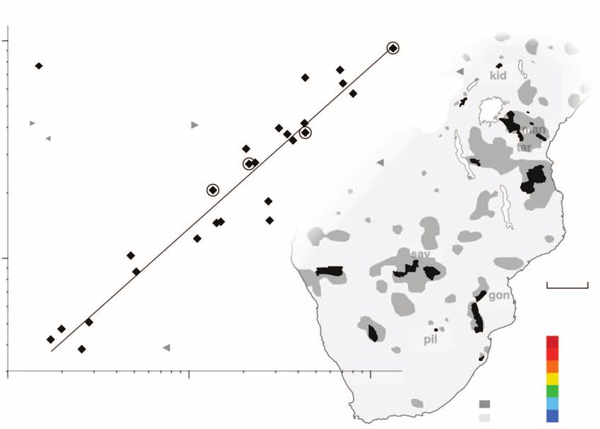
R ES E A RC H

                                                ◥                                                                            We began by considering the predator-prey
    RESEARCH ARTICLE                                                                                                     biomass power law in African savanna, shown
                                                                                                                         in Fig. 1, which serves to identify key properties
                                                                                                                         of this more general phenomenon. The pattern
MACROECOLOGY                                                                                                             describes relative changes in the shape of the
                                                                                                                         “Eltonian” pyramid of biomass, which represents

The predator-prey power law:                                                                                             how total biomass is distributed across com-
                                                                                                                         munities at different trophic levels in the food
                                                                                                                         chain (43–45). In any given environment, the
Biomass scaling across terrestrial                                                                                       pyramid often exhibits a consistent shape, called
                                                                                                                         the trophic structure, but in different environ-

and aquatic biomes                                                                                                       ments, the same communities of species may be
                                                                                                                         in quite different relative proportions (39–42).
                                                                                                                         That is, pyramid shape may change with size,
Ian A. Hatton,1* Kevin S. McCann,2 John M. Fryxell,2 T. Jonathan Davies,1                                                which can be described by the predator-prey
Matteo Smerlak,3 Anthony R. E. Sinclair,4,5 Michel Loreau6                                                               power law exponent k.
                                                                                                                            Power laws are simple functions of the form
Ecosystems exhibit surprising regularities in structure and function across terrestrial and                              y = cx k, where c is the coefficient (y value at x = 1)
aquatic biomes worldwide. We assembled a global data set for 2260 communities of                                         and k is the dimensionless scaling exponent (1, 2).
large mammals, invertebrates, plants, and plankton. We find that predator and prey                                       On logarithmic axes, power laws follow a straight
biomass follow a general scaling law with exponents consistently near ¾. This pervasive                                  line with slope k but on ordinary axes may curve
pattern implies that the structure of the biomass pyramid becomes increasingly                                           up (k > 1) or down (k < 1). The slope k of the
bottom-heavy at higher biomass. Similar exponents are obtained for community                                             relation of the log of predator biomass versus the
production-biomass relations, suggesting conserved links between ecosystem structure                                     log of prey biomass identifies the relative change
and function. These exponents are similar to many body mass allometries, and yet                                         in the shape of the pyramid (Fig. 2). An exponent
ecosystem scaling emerges independently from individual-level scaling, which is not                                      k > 1 means that the pyramid becomes relatively
fully understood. These patterns suggest a greater degree of ecosystem-level organization                                more top-heavy at higher biomass and is pre-
than previously recognized and a more predictive approach to ecological theory.                                          dicted by top-down control of predators on prey
                                                                                                                         (41, 42, 46–48) (appendix S1). An exponent k = 1

M
                                                                                                                         indicates that pyramid shape remains constant
         any large-scale patterns in nature follow            pattern occurs, because it is not predicted by             and is predicted by bottom-up control, whereby a
         simple mathematical functions, indicat-              current theoretical models and, as far as we can           constant fraction of biomass is produced and
         ing a basic process with the potential for           detect, is unexpected from lower-level structure.          transferred to each successively higher trophic
         deeper understanding (1). When the same              What is surprising is that the same pattern                level (8, 41, 42, 49) (appendix S1). Last, k < 1 in-
         pattern recurs in different kinds of sys-            recurs systematically in different places, includ-         dicates that the pyramid becomes relatively more
tems, it urges consideration of their shared prop-            ing grasslands, forests, lakes, and oceans. Our            bottom-heavy at higher biomass (Fig. 2).
erties and provides the opportunity for synthesis             analysis has its basis in empirical data drawn                We show that the shape of the predator-prey
across systems (2). Ecology has increasingly ob-              from more than 1000 published studies, many                biomass pyramid becomes systematically more
served patterns over very large scales and across             of which are cross-system meta-analyses (9–33)             bottom-heavy as pyramid size increases along a
levels of organization, from individuals and pop-             (materials and methods, section M1, A to C). In            biomass gradient. Similar changes are also ob-
ulations to communities and whole ecosystems                  total, we bring together biomass and production            served for per capita productivity with biomass,
(3–8). These patterns depict the boundaries in                measurements for tens of thousands of pop-                 suggesting a basic link between aspects of eco-
which life exists and are often highly conserved              ulations over 2260 ecosystems in 1512 distinct             logical structure and function. Our findings thus
across taxa and types of communities. This points             locations globally. Our approach is similar to a           reveal highly conserved patterns in pyramid size,
either to intrinsic characteristics of the individ-           number of other large-scale cross-system meta-             shape, and growth across different kinds of eco-
ual, such as shared ancestry or energetic con-                analyses (10, 19–21, 29–42), allowing compari-             systems. In particular, community production-
straints (5, 6), or else extrinsic factors, such as the       sons to previous work.                                     biomass scaling is commonly near k = ¾ across
way that many individuals are aggregated, grow,
and interact (1, 7). The challenge in ecology, as in
many fields, is to link large-scale patterns to               Fig. 1. African predator-prey
finer-grain processes (1, 4).                                 communities exhibit sys-
   Here, we present a pattern that follows a sim-             tematic changes in ecosys-
ple function and recurs across a variety of eco-              tem structure. Predators                                 y = 0.094x 0.73
                                                                                                           100

system types in different biomes worldwide. The               include lion, hyena, and other                           R2 = 0.92
pattern is only observed over large aggregations              large carnivores (20 to                                  n = 46
of individuals and appears to emerge uniquely at              140 kg), which compete for
the ecosystem level. We do not know why this                  large herbivore prey from        Predator
                                                                                               biomass
                                                              dik-dik to buffalo (5 to
                                                                                                           10

1
 Department of Biology, McGill University, Montréal, Québec   500 kg). Each point is a         (kg/km2)
H3A 1B1, Canada. 2Department of Integrative Biology,          protected area, across which
University of Guelph, Guelph, Ontario N1G 2W1, Canada.
3                                                             the biomass pyramid
  Perimeter Institute for Theoretical Physics, Waterloo,
Ontario N2L 2Y5, Canada. 4Biodiversity Research Centre,       becomes three times more
University of British Columbia, Vancouver, British Columbia   bottom-heavy at higher
V6T 1Z4, Canada. 5Tanzania Wildlife Research Institute,
                                                                                                           1

                                                              biomass. This near ¾ scaling
P.O. Box 661, Arusha, United Republic of Tanzania. 6Centre                                                       100                1000               104
                                                              law is found to recur across
for Biodiversity Theory and Modeling, Experimental Ecology
Station, CNRS, 09200 Moulis, France.                          ecosystems globally.                                         Prey biomass (kg/km2)
*Corresponding author. E-mail: i.a.hatton@gmail.com

SCIENCE sciencemag.org                                                                                            4 SEPTEMBER 2015 • VOL 349 ISSUE 6252          aac6284-1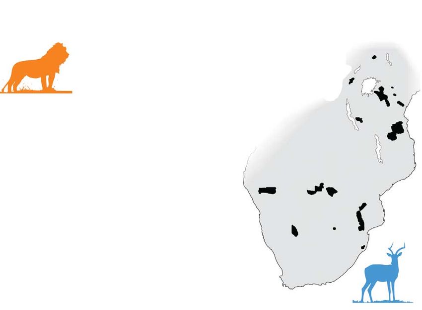
R ES E A RC H | R E S EA R C H A R T I C LE

different types of ecosystems and is thus curious-                                 0.92; Fig. 1). Data derive from 190 studies that                                            formed to the predator-prey biomass ratio, giving
ly similar to individual production-body mass                                      reported population density in 23 protected                                                 a null exponent k = 0. In contrast to the null hy-
allometry. This may suggest a similar process                                      areas at different points in time (section M2A).                                            pothesis, the observed predator-prey biomass
recurs across levels of organization.                                              These counts cover the dominant species of large                                            ratio exhibits highly significant declines (P value
                                                                                   carnivores (wild dog, cheetah, leopard, hyena,                                              < 10−9), a pattern that has been observed inde-
Why are there not more lions?                                                      and lion) and their characteristic herbivore                                                pendently in separate studies (9–12) and is ro-
Across African savanna ecosystems (Fig. 1), the                                    prey [5 to 500 kg; 27 species (50, 51)]. The pop-                                           bust to a variety of assumptions (section M2B).
total biomass of large carnivores follows a con-                                   ulation density (numbers of individuals per                                                 This pattern, however, cannot be predicted from
sistent relation to the total biomass of their                                     unit area) of these species vary over 3 to 4 orders                                         population or community structure (Fig. 3, A and
herbivore prey. The exponent is k = 0.73, which                                    of magnitude (Fig. 3A), but, when aggregated                                                B), and, as far as we are aware, there is no current
is sublinear (k < 1), and indicates that the trophic                               into trophic communities within their respec-                                               theoretical basis for expecting such changes in
pyramid becomes relatively more bottom-heavy                                       tive ecosystems, the variability collapses along                                            trophic structure (appendix S1). Large-mammal
at higher biomass. From the dry Kalahari desert                                    a highly regular power law (Fig. 1). The observed                                           time series over the past 50 years in several of
to the teeming Ngorongoro Crater, there are                                        change in pyramid shape is unexpected given                                                 these systems show that communities are near
threefold fewer predators per pound of prey,                                       that trophic communities maintain a near con-                                               steady state, even as component populations
which leads to the question: where prey are                                        stant size structure. The mean body mass, which                                             fluctuate and largely compensate with one an-
abundant, why are there not more lions?                                            is the total biomass divided by the total nu-                                               other, for a more regular central tendency at the
                                                                                   merical density (52), averages over all individ-                                            community level (section M2C). The predator-
Trophic structure in African savanna                                               uals and provides an indication of community                                                prey pattern thus appears to emerge uniquely at
The African predator-prey pattern is remark-                                       size structure. Both carnivore and herbivore                                                the ecosystem level by aggregating over large
ably systematic given how it is constituted (R2 =                                  mean body mass scale with biomass near ex-                                                  numbers of individuals.
                                                                                   ponents k = 0.03 (Fig. 3B), indicating that size
                                                              Top-heavy                                                                                                        Linking trophic structure and function
                                                                                   structure is nearly invariant and that both the
                                  Predator biomass
                                                                                   pyramids of biomass and the pyramid of num-                                                 If we cannot predict this pattern from lower-
                                  Prey biomass                   k>1
                                                                                   bers (numerical density) change in similar ways                                             level structure, what high-level function might
                                                                                   (section M2B) (43–45). Both the diversity and                                               be operating? What flux rates into or out of
                                                              Invariant            the frequency of different size classes are also                                            each trophic community may be shaping trophic
                                             Relative
                                                                                   nearly invariant, so that most species have sim-                                            structure? For systems near steady state, flux in
                                             change              k=1               ilar relative frequencies across the biomass                                                and out should balance, but flux rates may not
                                                                                   gradient (histograms in Fig. 3B). The carnivore-                                            be proportional to standing biomass. To inves-
                                                          Bottom-heavy             to-herbivore body mass ratio is thus constant                                               tigate the relation between pyramid shape and
                                                                                   even as their biomass ratio declines dramatically                                           trophic flux, we consider a simple predator-
                                                                 k
RE S E ARCH | R E S E A R C H A R T I C L E

        dC                               mC              to depend on the productivity of the prey com-           estimated with increasing error, alternative meth-
           = gQ mC                 C                     munity, which exhibits a systematic form of den-         ods (e.g., type II) tend to overestimate the exponent
        dt                               gQ              sity dependence, but also on the densities of other      (section M1D) and yet are also sublinear (k < 1)
                                                         predators, with which lions are compensatory. The        for all plots, except where data are highly dis-
         dB                               Q              regularity of this pattern suggests high-level organi-   persed [Fig. 5, F, G, and L; R2 < 0.5; k near 1;
            =P Q                   B                     zation and possibly complex regulatory pathways,         section M3; (65)]. Nonetheless, we cannot be
         dt                               P              which only more detailed study can elaborate.            certain of the exponent value, and even the best-
                                                         But how general are these structural and func-           studied ecosystem types do not extend much be-
Fig. 4. A predator-prey model (C, B) with two
                                                         tional patterns across other kinds of ecosystems?        yond a two order of magnitude biomass gradient,
functions (P, Q). Different models are specified
                                                                                                                  which may be insufficient to establish power
based on the functions for prey production P(B)          Biomass scaling globally                                 law behavior. Currently available data also do not
and prey consumption by predators, Q(B,C). Pred-
                                                         Predator-prey biomass scaling is not unique to           permit highly standardized community level mea-
ator production, gQ, depends on the growth ef-
                                                         the African savanna and is found to recur across         surements, so that different biomes may repre-
ficiency g in converting consumption into offspring.
                                                         a variety of other kinds of ecosystems. Our model        sent different levels of sampling and taxonomic
Predator loss is mC, where m is mortality rate.
                                                         suggests this pattern is underpinned by similar          resolution. Despite these limitations, however,
                                                         production-biomass scaling (Fig. 4). Although            declines in y/x versus x are highly significant for
we believe African large mammal communities              data are not available for the same ecosystems to        all variables in Fig. 5, A to O (all P values < 0.01).
to be near steady state (C*, B*), the predator-prey      test this connection directly, these two scaling         Similar scaling is also obtained for each of 25
power law can be expressed as                            relations exhibit similar exponents near k = ¾           published cross-system data sets (9–30, 66, 67);
                                                         across terrestrial and aquatic ecosystems. This          kavg = 0.72; ntot = 2950 ecosystems; section M3;
                      C* = cB*k                          suggests that a common community growth pat-             table S2), providing independent validation
                                                         tern may be shaping biomass pyramids across              of the pattern. Across terrestrial and aquatic
where c is the predator-prey coefficient (in Fig. 1,     distinct ecosystem types.                                ecosystems, therefore, the predator-prey ratio
c = 0.094 kg1 – k and k = 0.73). We thus seek P and                                                               and per capita production decline significant-
Q functions that give rise to this structural pattern.   Empirical findings                                       ly at higher biomass, both following similar
At equilibrium, both equations in Fig. 4 can be set      Predator and prey biomass follow a power law             scaling.
to zero, and we can substitute the prey equation         with a sublinear exponent (k < 1) across several
(Q* = P*) into the predator equation (C* = gQ*/m)        terrestrial and aquatic biomass gradients. Tiger         Theoretical implications
(where g is the predator growth efficiency and m is      and wolf biomass over their respective conti-            Several cross-system meta-analyses, using simi-
the predator mortality rate), giving C* = gP*/m. To      nents both scale to prey biomass with exponents          lar methods to our own, have shown that herbi-
obtain C* = cB*k above, prey production may scale        near k = ¾ (Fig. 5, C and D) (13–17). These car-         vore consumption scales near linear (k = 1) to
in the same way with prey biomass, which can be          nivores represent a dominant part of the large           primary production (34–37) (section M3Q and
expressed as                                             predator community, comparable to lion and               table S5). This implies that flux rates into and
                                                         hyena populations (Fig. 5, A and B). Similarly,          out of basal communities are roughly propor-
                       P = rBk                           zooplankton and phytoplankton biomass follow             tional across productivity gradients, which may
                                                         near ¾ scaling patterns across lakes and oceans          be expected for systems near steady state. To-
Here r is the prey production coefficient (units         and through time (Fig. 5, E to H) (18–22). A num-        gether with these earlier studies (34–37), our
kg1 – k/time), and k is assumed to be 0.73. The          ber of studies have reported the same qualitative        empirical findings have implications for eco-
predator-prey coefficient is thus                        declines in predator-prey ratios across diverse en-      logical theory.
                                                         vironments (14, 17, 19–22, 38, 40–42, 58–64) (sec-          1) Predator-prey scaling is sublinear (Fig. 5,
                      c = rg/m                           tion M3), suggesting a widespread phenomenon.            A to H), which indicates that trophic structure
                                                            Similar scaling is also observed for commu-           is more bottom-heavy at higher biomass. At
   Regardless of how consumption Q is speci-             nity production-biomass relations in grasslands          steady state, this can be expressed as C* = cB*k,
fied, trophic structure should depend on lower           (23–25), broadleaf and coniferous forests (26–28),       where c is the predator-prey coefficient and k < 1.
trophic productivity, P, according to a simple           seagrass beds (29), and algal (18) and inver-            This equilibrium solution is at odds with com-
relation of flux rates. On the left of the equality      tebrate communities (30) (Fig. 5, I to O; sec-           mon models that assume that prey production
is the predator-prey coefficient c, which influ-         tion M3, I to O; and table S1). Exceptions to            P follows logistic density dependence. These
ences pyramid shape, whereas on the right are            this pattern exist where multiple trophic groups         models are often classed as top-down or bottom-
parameters for flux rates into and out of each           are combined. Fish (Fig. 5P), for example, com-          up control according to how Q is specified and
trophic community. Clearly, the dynamic inter-           bine benthivores and planktivores, as well as            predict more top-heavy (k > 1) or invariant (k = 1)
actions of five carnivore species and many more          piscivores, at a higher trophic level (31, 32). Al-      pyramid structures with increasing biomass
species of prey across vast areas of the conti-          though data are few, when these trophic groups           (8, 41, 42, 46–49) (appendix S1). Classic models
nent cannot be captured by two differential equa-        are considered separately, lower-trophic groups          can be reconciled with data by introducing the
tions. This coarse-grained description, however,         scale sublinearly [k ranges from 0.74 to 0.81            production function described below (2).
focuses on a few key flux rates and brings dy-           (33)], whereas piscivores exhibit near-linear scal-         2) Production-biomass scaling is sublinear
namical perspective to the question of what is           ing (k = 1.1; section M3P). It is possible that          (Fig. 5, I to O) and indicates that per capita
shaping trophic structure. We have tested this           piscivores are dominating the pattern in Fig. 5P,        growth declines at higher biomass. For prey,
theoretical prediction (c = rg/m) for African large      although data among higher trophic levels are            this can be expressed as P = rBk, where r is the
mammals, estimating their community rate pa-             generally limited.                                       production coefficient and k < 1. This production
rameters (r, g, and m) independently from the               This pattern is largely robust to regression          function theoretically yields observed predator-
fitted coefficient in Fig. 1, and find close corre-      methods and is validated by independent data             prey scaling (Fig. 4) and implies that, in the
spondence (appendix S2). This suggests a link            sources. Previous cross-system studies have re-          absence of predators, prey increase if food is
between trophic structure and the production             ported exponents fit by ordinary least squares           available, but with an ever-diminishing tenden-
function. Specifically, where prey are abundant,         (10, 19–21, 29–42). As far as we can determine,          cy. This is a weaker form of density dependence
they appear to reproduce at consistently lower           this is the least biased regression method for           than logistic, but systematic and possibly scale-
rates, which in turn influences the biomass of           the data that we report (section M1D). Although          free. Model stability is thus found to be exten-
predators. Lion abundance, for example, appears          least squares exponents are increasingly under-          sive in parameter space for different Q functions

SCIENCE sciencemag.org                                                                                       4 SEPTEMBER 2015 • VOL 349 ISSUE 6252       aac6284-3
R ES E A RC H | R E S EA R C H A R T I C LE
Lion, tiger & wolf
combined range:
Present
Historic
Predator-prey scaling A Lion-prey B Hyena-prey C Tiger-prey D Wolf-prey
0.1
k = 0.77 k = 0.74 k = 0.74 k = 0.72
Predator (g/m2)
0.01
3
10
Top-carnivore biomass vs
total herbivore prey biomass
4
10
k = 0.74 (0.68, 0.81), n = 184 0.1 1 10 0.1 1 10 1 0.01 0.1 1
E Freshwater F English Channel G Atlantic Ocean H Indian Ocean
100
k = 0.66 k = 0.73 k = 0.73 k = 0.70
Predator (g/m3)
1
0.01
Zooplankton biomass vs total
algal community biomass
4
10
k = 0.71 (0.65, 0.76), n = 667 0.1 1 10 100 0.1 1 10 0.1 1 10 3
0.01 0.1 1
Prey biomass (A-D: g/m2 , E-H: g/m3)
Production-biomass scaling I Grassland, total J Grass above-ground K Broadleaf forest L Coniferous forest
Production (g/m2/yr)
4
10
k = 0.71 k = 0.67 k = 0.66 k = 0.67
3
10
100
Plant community production
vs total foliage biomass
k = 0.67 (0.64, 0.71), n = 1153 100 103 104 100 103 100 103 103
M Seagrass N Algae, lakes O Zooplankton, lakes P Fish, lakes & rivers
Production (g/m2/yr)
k = 0.64 k = 0.70 k = 0.74 k = 1.09
4
10
100
Aquatic trophic community
1
production vs total biomass
0.01
k = 0.76 (0.68, 0.83), n = 256 1 10 100 103 1 10 100 0.01 1 100 1 10 100
Community biomass (I-P: g/m2)
Fig. 5. Similar scaling links trophic structure and production. Each point is an ecosystem at a period in time (n = 2260 total from 1512 locations)
along a biomass gradient. (A to P) An exponent k in bold (with 95% CI) is the least squares slope fit to all points n in each row of plots. Further details are
in section M3 and table S1.
aac6284-4 4 SEPTEMBER 2015 • VOL 349 ISSUE 6252 sciencemag.org SCIENCERE S E ARCH | R E S E A R C H A R T I C L E
(see supplementary text), suggesting that this munities, especially among algae (Fig. 8, D to F) biomass gradient are largely due to increases
growth pattern may help to balance trophic in- (22, 31, 32, 52). For biomass scaling to be the in population density. Increases in biomass
teractions across large-scale gradients. direct result of body mass allometry, we expect may also be due to increases in diversity but
3) The similarity of predator-prey (item 1) mean body mass to scale with biomass near k = 1. are never solely due to changes in body size.
and production-biomass (item 2) scaling im- Changes in plankton size structure, therefore, are 3) Per capita declines in community produc-
plies a broadly conserved link between these not sufficient to account for changes in trophic tion are largely due to density-dependent de-
structural and functional variables. Although structure or per capita productivity. We can thus clines in individual productivity from their
our model (Fig. 4) is only a phenomenological deduce the following (which only partly holds for maximum potential, shown in Fig. 6.
description of trophic dynamics, it may pro- plankton communities). Size structure thus suggests that the scaling
vide a first approximation for the link between 1) Ecosystem and individual near ¾ expo- of individual maximum production is indepen-
these two power law coefficients (c = rg/m), nents appear to arise independent of changes dent from that of community production. Instead,
allowing variables in Fig. 5 to be reformulated in size structure. Mean body mass is poorly cor- individual production appears to systematically
in terms of one another for more extensive pre- related to community biomass, indicating that decline from its maximum (Fig. 6), with increases
dictions (e.g., appendix S2). Theory and data thus their mass exponents are not directly related. in the density of the community in which it re-
point to a general community growth pattern 2) Increases in community biomass along a sides. We therefore expect to observe maximum
that shapes trophic structure in terrestrial and individual production only at very low densi-
aquatic systems. ties, where we can make predictions for com-
But where does this growth pattern originate? munity production from individual data. At
Although we cannot be certain of the exponent 108 y = 3.5x 0.75 higher densities, however, community produc-
Maximum production (g/yr)
value, ecosystem-level scaling is often near k = ¾ R2 = 0.98 tion will likely be overestimated unless density
104
and evokes a link to individual-level body mass n = 1635 dependent declines in individual production are
allometry. Many vital characteristics of an indi- accounted for. Assuming a biomass exponent
vidual scale with body mass near k = ¾ (68),
1
including metabolism (5, 6), production (69–72),
and consumption (9, 52, 57). This means that, as Ecosystem Individual
4
k
10
a body enlarges within a species or across taxa, 1
Mammal
these rates decline on a per mass basis. Near ¾ Protist Mammal
8
10
body mass exponents appear to be physiologi- Plant Protist
0.75
cally linked and are widely thought to be ener- Ectotherm Plant
12
getically constrained (5–7, 71–76). Here, however, Ectotherm
10
we are considering aggregations of many in- 10 12
10 8
10 4
1 104 108 All 0.5 n = 2156 n = 1635
dividuals across separate ecosystems, and so Individual body mass (g) Fig. 7. Ecosystem and individual growth patterns
it is not clear how the same energetic constraints
Fig. 6. Individual production to body mass ex- are similar. Least squares exponents k (and 95%
would apply. Unlike the similarity between predator-
hibits near ¾ scaling across taxa. Maximum in- CI) for production-mass across ecosystems (from
prey and production-biomass scaling, which has
dividual production includes somatic growth and Fig. 5) and individuals (from Fig. 6) are often near
some theoretical basis (implication 3, above),
offspring production. Each point is an individual, k = ¾. Each exponent estimate is for n > 100
the similarity between ecosystem and individual
representing 1098 species over 127 taxonomic or- data points. Seagrass data (n = 104; Fig. 5M) were
scaling does not.
ders. Further details are in section M4 and table S3. excluded. Further details are in section M4.
Links to lower levels
Community production and biomass repre-
sents the total individual production and total Mammal carnivores Mammal herbivores Forest trees
body mass summed over all individuals within k = -0.02 (N.S) k = 0.25 (N.S)
k = -0.04 (N.S)
106
the community, and so we consider the indi-
107
105
vidual production allometry. From microscopic
algae up to elephant, maximum individual pro-
105
105
duction exhibits highly robust near ¾ scaling with
50 kg
Mean body mass (g)
body mass (Fig. 6 and section M4) (5, 6, 68–76).
Individual and community production scaling
104
103
are thus notably similar, and although there are 0.01 0.1 0.1 1 10 100 103
important exceptions, such as for individual pro-
tists (77), this parallel tends to hold across major Freshwater fish Lake zooplankton Marine algae
taxa (Fig. 7) (tables S1 to S3). But maximum in-
k = -0.27 (N.S) k = 0.29 k = 0.56
1 kg
dividual growth is not the actual individual growth
4
9
10
within a community, and so this apparent simi-
10
larity may be misleading.
5
10
10
10
10
Deductions from size structure
11
To connect ecosystem- to individual-level pro-
6
0.1
10
10
cesses, we examine community size structure
1 10 0.1 1 10 0.1 1 10
(Fig. 8) and specifically mean body mass versus
total biomass (52) (section M5). As in African Community biomass (A-D: g/m2 ; E-F: g/m3)
ecosystems (Fig. 3B), we find that size structure Fig. 8. Mean body mass is poorly correlated to community biomass except in plankton. Points are
shows few systematic changes across large mam- mostly the same as those in Fig. 5. Mean body mass averages over all individuals in a community. The
mal and forest biomass gradients (Fig. 8, A to C) slopes k in (A) to (D) are not significant (N.S; all R2 < 0.05), but plankton size structure varies positively
(13–16, 26, 27). In contrast, at higher aquatic with biomass (E and F). Mammal systems (A and B) include data from Fig. 3B. Further details are in
biomass, mean size increases in plankton com- section M5 and table S4.
SCIENCE sciencemag.org 4 SEPTEMBER 2015 • VOL 349 ISSUE 6252 aac6284-5R ES E A RC H | R E S EA R C H A R T I C LE
near k =¾ allows community-level predictions Community growth scaling emerges over large Biomass density was converted to kg/km2
from individual-level data across a biomass gra- numbers of individuals and size structure is often for Figs. 1 and 3 and to g/m2 or g/m3 for Figs. 5
dient (appendix S2). near constant, indicating that similar growth and 8. Changing units for all data in a plot in a
dynamics at the community and individual levels consistent way has no effect on the scaling ex-
Outlook arise independently (Fig. 8). This may point to ponent but will alter the coefficient. However,
Size-structure suggests unique emergence of basic processes that reemerge across systems the use of different conversion factors for dif-
growth scaling at the community and individual and levels of organization. ferent meta-analyses combined in the same plot
levels, and, although we can make high-level pre- can affect both the exponent and the coefficient.
dictions from lower-level function, we do not Materials and methods For example, each of Fig. 5, E, I, and J, combines
know why growth patterns at different levels A description of our empirical approach and data multiple meta-analyses, some of which are re-
are so markedly similar. Models for individual (Figs. 1 to 5) is outlined below (sections M1 to ported in fresh mass, whereas others are in dry
growth scaling going back to the well-known M5). Materials and methods are supplemented mass. We used conversion factors reported in
Bertalanffy model assume a dependence on with regression tables S1 to S5 and appendices S1 the original studies to normalize data to a con-
metabolic scaling (73–76). Although our model and S2 (supplementary materials file), as well as sistent set of units. Where conversion factors
for prey community growth (Fig. 4) resembles raw data and original sources in the data file were not reported, we converted all dry mass or
these ontogenetic growth models, we cannot (database S1), and are available at Science Online. mass of carbon to fresh mass by multiplying by
assume the same metabolic rationale. Commu- a factor of 10 (68). In these instances, we tested
nity growth scaling arises over large aggrega- M1. Empirical approach whether each meta-analysis yielded similar ex-
tions of individuals that often change little in A. Criteria for inclusion in the database ponents in isolation; all of them were found to
their size structure, which leads us to wonder This study focuses on how ecological structure be within 0.1 of exponents from combined meta-
not only what underpins this pattern in differ- and dynamics change across ecosystems made of analyses. Exponents reported in Fig. 5 are thus
ent ecosystems, but how might it recur across similar species assemblages. This requires data representative of the individual studies they
levels of organization. gathered consistently by different studies across comprise (table S2).
Density-dependent growth has been observed large-scale biomass gradients. We focused on rel-
over thousands of populations in diverse taxa atively distinct trophic communities, rather than C. Methods for estimating biomass
(78, 79) and is qualitatively consistent with this ecosystems with more complex feeding relation- and production
growth pattern. Population density is known to ships. This restricted the kinds of ecosystems Community biomass is the total mass density
influence physiology, community composition, that could be considered to currently available summed over all individuals in a given trophic
and competition for space. Density-dependent data on large mammals, plants, and basal aquatic level community (e.g., g/m2). Production is the
factors can alter reproductive behavior, life history, communities. total increase in biomass per unit time (e.g., g/m2
and metabolism (80, 81); promote self-shading All data were sourced from peer-reviewed per year), in the absence of consumption, which
and self-thinning (82, 83); cause changes in size publications and met the following criteria: has the same units. Methods for estimating com-
structure and nutritional quality (36–41, 84–86); (i) Ecosystems were relatively free of human in- munity biomass and production are not equiv-
and trigger interference and territorial aggres- fluence or disturbance and were thus repre- alent across ecosystem types, nor are they always
sion (87, 88). What is not known is whether these sentative of natural conditions. (ii) Ecosystems equivalent across biomass gradients of similar
factors can account for observed scaling expo- were surveyed over a much larger area than the species (Fig. 5). The same is true for body mass
nents, and whether these different factors may largest animal home range, so that density es- and individual production across the size spec-
have similar effects when aggregated across whole timates were not biased because of local aggre- trum (Fig. 6). Details of methods can be found in
communities. The generality of community-level gation. (iii) Communities comprised the majority the original studies and summarized in the rele-
scaling suggests a process that operates in regular of dominant species and were thus representa- vant places cited in database S1. A summary of
ways and independently of system details. A the- tive of whole trophic communities. Noted excep- methods for biomass and production measure-
ory for growth-mass scaling encompassing both tions include predator communities in Southeast ments at the ecosystem level can be found in
individual and ecosystem levels would efficiently Asia and North America, represented by a single Cebrian and Lartigue (37) and at the individual
unite basic aspects of physiology and ecology. top-predator population (Fig. 5, C and D, tiger level in Ernest et al. (71).
and wolf), and zooplankton communities in the Despite attempts of different studies to es-
Conclusion Atlantic and the Indian Ocean, represented only timate the same variables in standardized con-
Ecosystems exhibit emergent regularities in by micro-zooplankton (Fig. 5, G and H). These vertible units, combining data obtained through
trophic structure and production dynamics across predators are reported to be the dominant con- very different methods can cause inaccuracies in
terrestrial and aquatic biomes of the world sumers of prey biomass in their respective eco- the scaling exponent. This is particularly true if
(Fig. 5). The predator-prey ratio and per capita systems (14, 17, 22). there are any systematic biases across a bio-
community production both significantly decline mass gradient. Many inaccuracies will likely be
at higher biomass. Both of these relations follow B. Conversion of raw data into relatively small compared with the near two
similar power law scaling, which suggests a con- standard units orders of magnitude over which many relations
served link between ecosystem structure and Many of the meta-analyses that were combined extend. Nonetheless, this was an important con-
function across diverse systems. Often these for this study reported data in different units. sideration for treating ecosystem types sepa-
patterns are highly regular (e.g., Fig. 1), implying Conversion into standard units required par- rately, where the most substantial divergences
a greater degree of ecosystem-level organization ticular care, especially among aquatic systems, in methodology exist.
than previously recognized and raising ques- where mass variables may be reported in fresh
tions about the processes that regulate abundance or dry mass (picograms to tons) and density D. Regression method
in ecological communities. We show how sub- may be reported in areal or volumetric units. Ordinary least squares (OLS) was used for all
linear growth scaling tends to stabilize predator- We avoided changing density dimensions (e.g., fits to log-transformed data, consistent with
prey interactions (supplementary text), but further area to volume) in all but one case (one of four a number of other published cross-ecosystem
work is needed to understand how specific fac- meta-analyses used in Fig. 5E), where the au- meta-analyses (10, 19–21, 29–42). However,
tors operate in different systems. thors made clear how the data were estimated there is ongoing debate about which regression
Perhaps the most intriguing aspect of these and provided mean lake depth, allowing con- methods are least biased depending on the dis-
findings is that community and individual growth version of mass per unit area into mass per tribution of error between x- and y-axis varia-
patterns both follow near ¾ scaling laws (Fig. 7). unit volume (18). bles (65, 89–96). OLS (type I) is the standard
aac6284-6 4 SEPTEMBER 2015 • VOL 349 ISSUE 6252 sciencemag.org SCIENCERE S E ARCH | R E S E A R C H A R T I C L E
approach in fitting bivariate power laws in ues obtained by using RMA and MA are discussed highest prey biomass. The four herbivore size
biology (68, 95), but it assumes all error is in further in section M3. classes are 5 to 20, 20 to 50, 50 to 200, and 200
the y variable and thus tends to underestimate The relations shown here are bivariate, so to 500 kg. The three carnivore size classes are
k as error in x increases. Type II regression that much of the statistical literature on power the three smallest carnivores combined (wild dog,
methods, such as reduced major axis (RMA) law fitting of univariate rank-frequency distri- leopard, and cheetah; 20 to 40 kg), hyena (50 kg),
and major axis (MA), partition error to both butions may be less relevant (107, 108). Each and lion (125 kg). The slight change in some her-
axes but can overestimate k as the error in y axis variable was gathered independent of the bivore size classes is small relative to the changes
increases relative to x (65, 91, 93–96). other, often using different methodologies, and in trophic structure shown in Figs. 1 and 3C.
We assumed OLS to be the least biased slope so there is no possibility that the strength of The predator-prey biomass scaling pattern
estimator for the specific data that we report, these patterns is due to indirectly regressing a shown in Fig. 1 and their ratio in Fig. 3C includes
given the greater fraction of error associated variable against some proxy of itself (109). the five dominant African carnivores (lion, spotted
with y-axis variables compared with x-axis var- hyena, leopard, cheetah, and wild dog), which
iables. Mammal predators, such as lion, hyena, M2. African savanna data (Figs. 1 and 3) compete for prey ranging from 5 to 500 kg (50, 51).
tiger and wolf (y axis, Fig. 5, A to D), are con- The African savanna data set includes complete In the Savuti region of Chobe NP, mega-herbivores
siderably more difficult to census than their prey large mammal abundance estimates assembled (>750 kg) are frequently preyed upon by lions in
(x axis) because of their often nocturnal habits across whole ecosystems. Most systems were the dry season (116) and were included as prey
and relatively low densities, which cause greater censused over the entire extent of the protected in this ecosystem (Fig. 9). We excluded the mi-
potential for estimation error (14, 60, 97, 98). Top area, which were only included in the database grant population biomass of wildebeest, zebra,
carnivores were also enumerated as single pop- if all dominant large mammals (>5 kg) were and gazelle in regions such as the Serengeti eco-
ulations that are likely compensatory with other counted. Data were checked against other pub- system and Masai Mara GR, which are known to
dominant guild members. The African savanna lished estimates, particularly for carnivore counts, largely escape predators, but nonetheless provide
data shown in Fig. 1 are an exception because where errors can most influence the fit (section important prey subsidies to carnivores (117). Ex-
they estimate the entire community of large pred- M1D). On average, 22 species from a pool of 40 cluding migrant biomass, Serengeti and Masai
ators. Here, the exponent remains nearly un- were estimated in each system, for a total of 1000 Mara become the largest outliers above the best
changed from OLS (k = 0.73) to MA (k = 0.75) large mammal abundance estimates drawn from fit line (Fig. 9), possibly because of the exclusion
and RMA (k = 0.76), but for individual lion and 190 published sources (Fig. 3A). of these subsidies. The largest outlier below the line
hyena to prey (Fig. 5, A and B), type II methods is in Katavi NP (Fig. 9), where previous research
give exponents near k = 0.88. Similarly, zoo- A. African ecosystem attributes has also reported relatively few predators (118).
plankton community biomass (y axis, Fig. 5, E The distribution of African protected areas span
to H) tends to be less well estimated than that the savanna rainfall gradient, from Kalahari des- B. Robustness of the African
of phytoplankton (x axis), because zooplankton ert to Ngorongoro Crater (Fig. 9). The relation- predator-prey pattern
aggregate and migrate in the water column (99). ship of log rainfall to log herbivore biomass has The African predator-prey pattern appears to
Estimating their biomass requires separate tech- been shown to yield significant slopes between be robust to the following: (i) how ecosystems
niques for different components of the com- k = 1.5 and 2.0 (10, 110, 111). Our data include a are replicated at different time periods, (ii) what
munity [e.g., crustacean, rotifer, and protozoan large proportion of ecosystems where other species are included in predator and prey com-
(22, 100)], whereas phytoplankton measurements sources of water dominate, which obscures the munities, (iii) variations in species body mass,
tend to converge on similar values (99, 101, 102). rainfall-to-herbivore relationship [Lake Manyara (iv) possible systematic bias in sampling, and
For the Atlantic and Indian Ocean (Fig. 5, G and National Park (NP), Tarangire NP, the Okavango (v) alternative regression approaches. These con-
H), macrozooplankton data were not available, Delta, Amboseli NP, and the area around Sabie siderations are elaborated further below.
and so the y-axis variable is also a partially in- River in Kruger]. The 23 analyzed regions range 1) Predator and prey biomass were fit to 23
complete community measure. in area from 100 to 40,000 km2, totaling more protected areas, some of which were sampled
Error is thus likely greater in the y axis for than 150,000 km2, over which census counts in different decades for a total of n = 46 eco-
predator-prey relations (Fig. 5, A to H), and the were made. Protected area map boundaries are system time periods. Replicate time periods are
same is true for production-biomass relations from (112), and lion range from (113). averaged in Fig. 9 (and Fig. 10A) to give equal
(Fig. 5, I to P). As a dynamic variable, produc- The relation of mammal abundance to body weighting to each area. Tarangire NP is the only
tion has the additional dimension of time over mass is highly variable across and within Af- system not averaged given large biomass fluc-
standing stock biomass and should control or rican protected areas (Fig. 3A). Mammal pop- tuations between wet and dry seasons in 1962 and
account for consumption and decomposition ulation density has previously been shown to 2000. The resultant fit is very similar to Fig. 1 (k =
between time intervals (44). Moreover, produc- scale with body mass by a negative exponent 0.75; n = 25 protected ecosystems R2 = 0.93), sug-
tion measurements often use a variety of tech- between k = –1 to –½ [also known as Damuth’s gesting there are no biases from possible pseudo-
niques that can give significantly diverging values law, or size-density scaling (5, 56, 68, 114)]. This replication.
[grasslands (103), forests (104, 105), aquatic in- size-density scaling relation extends over six 2) The pattern holds under alternative as-
vertebrates (106)]. For data in Fig. 5, the majority orders of magnitude in body mass and also sumptions about the breadth of the prey com-
of measurement error is in the y-axis variable, reveals that individuals of all size classes typ- munity. We excluded mega-herbivores from the
and therefore exponents derived from OLS are ically range in density over about three orders prey community, although carnivores will con-
expected to provide the most robust predictions of magnitude. This high residual variation re- sume juveniles and carcasses of mega-herbivores,
of the three regression approaches. sults in insignificant size-density correlations over such as giraffe and elephant. Including mega-
The precise distribution of error among axes a limited range in body size, as in Fig. 3A, even herbivores as prey in all ecosystems slightly reduces
remains difficult to ascertain. Reported k values compensating for possible undercounting smaller the exponent and goodness of fit but is otherwise
likely underestimate the exponent, and all the animals [e.g., a factor of 10; page 91 of (115)]. quite similar (k = 0.66; R2 = 0.65; Fig. 10C).
more so as error increases. An RMA exponent Populations in Fig. 3A were aggregated into 3) The pattern is robust to variations in species
can be estimated by dividing the OLS k value by their respective ecosystems to study the size body mass. Given that community composition
the square
pffiffiffiffiffiffi root of the coefficient of determina- structure of each trophic community across dif- is largely invariant across the prey biomass gradient
tion ( R2 ) (65, 91). These statistics are listed in ferent ecosystems. Mean body mass is described (Fig. 3B), the sublinear scaling evident between
tables S1 to S5. The vast majority of analyzed further below, in section M5. The histograms in total predator and prey biomass is also evident for
data sets exhibit sublinear biomass scaling ex- Fig. 3B show the frequency of different size classes, numerical density (Fig. 10B; k = 0.63; R2 = 0.86)
ponents under all three methods. Exponent val- averaged for the six systems with lowest and and implies that the pattern is largely robust to
SCIENCE sciencemag.org 4 SEPTEMBER 2015 • VOL 349 ISSUE 6252 aac6284-7R ES E A RC H | R E S EA R C H A R T I C LE
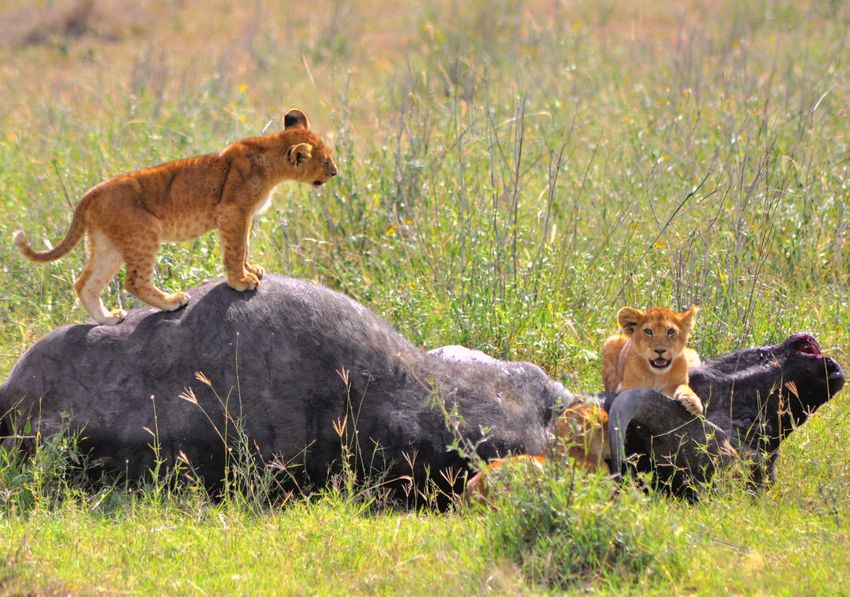
Fig. 9. African savanna
ecosystem characteris- African savanna ecosystems 04 78
100
tics. These data are shown 88 ngo
in Fig. 1, but here abun- 65
Ecosystem average
dance in different time 03 mas sab masMig kid
73 Replicate year (1973) 92 70 97
periods are averaged to give amb
W Wet season census
equal weight to each man
Total predator biomass (kg/km2)
D Dry season census 76 92 mas
sav que ser nai
protected area (k = 0.75 ; amb
95% CI = 0.66, 0.83;
Elx Elephants excluded savElx nai 6682
D W
man
Mig Migrants included nwa 00 ngo
n = 23). We excluded sel tar00Dhlu
03 93 tar mko
02
migrant biomass in Serengeti ser pil serMig
86 kat
and Masai Mara, which y = 0.08x 0.75 970975 77 sel
include the largest three R2 = 0.93 kru 84 71
outliers above the line (ser 64
que
and mas). Mega-herbivores
n = 25 oka
kid kat
were excluded as prey in all
but the Savuti region of tar62D
gon sav
10
96 eto oka
Chobe NP (sav), where hwa
lions prey on elephants 73 hwa 500 km
(116). When excluded from gon
Savuti, the point becomes W kru Rainfall
eto 98 kal nwa
a notable outlier (savElx). 26 D mko sab
(mm/yr)
The largest outlier below pil 250 -
tar62W kal kalMig
the line is Katavi NP (kat), hlu 350 -
where previous research 550 -
600 -
has reported relatively few 100 1000 104 Lion range 700 -
predators (118). Tarangire Present 800 -
Total prey biomass (kg/km2)
(tar) is not averaged due to Historic 1000 -
large biomass fluctuations.
Black circles are the
amb Amboseli NP kat Katavi NP que Queen Elizabeth NP
ecosystems in which time
eto Etosha NP kid Kidepo Valley NP nai Nairobi NP sab Sabie River
series data are shown
gon Gonarezhou NP kru Kruger NP ngo Ngorongoro Crater sav Savuti area of Chobe
in Fig. 10D.
hlu Hluhluwe-iMfolozi man Lake Manyara NP nwa Nwaswitshaka River sel Selous GR
hwa Hwange NP mas Masai Mara NR oka Okavango Delta ser Serengeti Ecosystem
kal Kalahari NP mko Mkomazi GR pil Pilanesburg NP tar Tarangire NP
assumptions about species body mass. Systematic yield exponents well within the confidence in- prey pattern exhibits greater dispersion, so that
changes in average species body mass exhibited by terval (CI) of the least squares fit (95% CI = 0.66 even dominant populations, such as lion versus
some mammals across ecosystems are never more to 0.79; major axis k = 0.75 and reduced major zebra or hyena versus impala, exhibit little or no
than a factor of two and thus not sufficient to axis k = 0.76; see section M1D). pattern (all R2 < 0.4 for population-level predator-
account for these sublinear scaling patterns. prey relations). Prey also exhibit compensation
4) Although it is possible that there are sys- C. Population compensation in space within any given ecosystem in time. Population
tematic biases of sampling one or both trophic and time biomass time series for lion and the six most
groups at high or low densities, this seems un- African mammal populations appear to be dominant African prey species were assembled
likely. The linear prediction of Carbone and compensatory in space and time, which allows across four large protected areas (Kruger NP,
Gittleman (53) is shown by the dotted line in greater regularity to emerge among whole com- Hluhluwe-iMfolozi NP, Serengeti ecosystem, and
Fig. 1 and Fig. 3C, which predicts that 111 kg of munities than among individual populations. Ngorongoro Crater; Fig. 10D). In nearly all cases
prey are needed for every 1 kg of predator. The For example, the community-level predator-prey the coefficient of variation (standard deviation
ecosystems that most distinguish the predator- pattern shown in Fig. 1 is not evident because divided by mean) is lower, indicating less fluc-
prey scaling relation from this prediction lie at fewer species are aggregated into the commu- tuation, for total prey community biomass than
the far left of the regression. Among these, five nity. Although the relations of lion and hyena to it is for the populations it comprises. This implies
whole-ecosystem censuses of all predators and total prey biomass give robust scaling patterns, that populations are compensatory in time (Fig.
prey were estimated by the same authors: Hwange they exhibit greater dispersion (Fig. 5A, R2 = 0.77, 10D), which is consistent with the emergence of
(119), Mkomazi wet and dry season (120), Tarangire and Fig. 5B, R2 = 0.69) than the whole predator the predator-prey pattern at the ecosystem-level.
wet season (121), and Kalahari (122). This suggests community pattern (Fig. 1, R2=0.92). In ecosys-
that similar censusing methods were applied to tems where lion are above the line, hyena tend to M3. Global community data (Fig. 5)
both predators and prey communities and that be below, and vice versa (Fig. 5, A and B). Given Community-level data aggregate many thousands
the deviation from a linear prediction is unlikely this compensation among predator populations, of population counts across 2260 ecosystems glob-
a result of bias. More generally, at least four in- higher R2 is obtained when lion and hyena are ally and are drawn from over 850 published sources,
dependent meta-analyses of a similar nature summed together and highest by further aggre- some of which include meta-analyses of addi-
have been conducted across African ecosystems, gating the large carnivore biomass of leopard, tional studies. Units were converted to g/m2 for
all of which yield similar sublinear patterns cheetah, and wild dog populations, all of which all terrestrial biomass data (Fig. 5, A to D and I
(9–12) (k ranges 0.67 to 0.80; Fig. 11A and compete for similar prey (50, 51). to L). Aquatic predator-prey data (Fig. 5, E to H)
table S2.1-4). Prey populations are also compensatory rela- were originally reported in various volumetric
5) Last, the scaling pattern is robust to alter- tive to predators. When fewer populations are units and converted to g/m3. All production-
native regression methods such as type II, which included in the prey community, the predator- biomass data, including aquatic studies (Fig. 5, I
aac6284-8 4 SEPTEMBER 2015 • VOL 349 ISSUE 6252 sciencemag.org SCIENCERE S E ARCH | R E S E A R C H A R T I C L E
Fig. 10. African mammal A Predator-prey biomass B Numerical density C Including megaherbivores
biomass, numerical
100
100
density relations, and y = 0.09x 0.75 y = 0.07x 0.63 y = 0.09x 0.66
Predator (kg/km2)
Predator (kg/km2)
Predator (N /km2)
1
population time series. R2 = 0.93 R2 = 0.86 R2 = 0.65
(A) This relation duplicates n = 24 n = 24 n = 24
Fig. 9 (colored according
to rainfall) to allow com-
10
10
parisons to the pyramid of
0.1
numbers (B) and prey
biomass including mega-
herbivores (C). Note that
Savuti is excluded and
100 1000 104 1 10 100 100 1000 104
Tarangire is not averaged 2 2
Prey biomass (kg/km ) Prey density (N /km ) Herbivore biomass (kg/km2)
for reasons outlined in
Fig. 9. (B) Predator-prey
total numerical density
shows a similar pattern Total prey biomass Buffalo Eland / kudu
because of the near D Population biomass timeseries (50 years) Lion biomass z Zebra Impala / gazelle
Elephant biomass w Wildebeest Various
invariance of mean body
mass with community kru hlu ser ngo
biomass (Fig. 3B). The
Pop. biomass (kg/km2)
4
lower exponent is driven w
wwwwwwwwww
w
10
w
ww w w ww
wwwwww w w ww
largely by two areas of z
zz
z zz zz
zz zz z
z
z zz z wzww wz z w
z z z
w
zz
z z z z zz z
z z
Kruger NP (sab and nwa;
1000
w
z
orange triangles) with high z w
z w z zz w zw
z zz
z z
ww w
w
zz zz zz zzz z z z z z z zzz ww
zz z
densities of impala. The zzz w w w ww
w
ww
z z
zz zzz zzz z zw www
z wwwww
ww w zzz
wwwww
wwwww ww w
z w
z z w z z
z z z ww z
ww
100
w w www w
exponent for all ecosystem w
ww w w
wwww
w
wwwwwwww
w
w www ww
ww
w
www wwww
w
time periods, omitting sab w
w
and nwa, is k = 0.70
10
(n = 42; R2 = 0.90).
64 75 84 97 09 82 00 71 77 86 93 03 65 78 88 97 04
(C) Predator to total her-
bivore biomass, including 1960 1980 2000 1960 1980 2000 1960 1980 2000 1960 1980 2000
all the prey in (A) plus all Year
mega-herbivores (giraffe to
elephant). The exponent for all ecosystem-time periods is k = 0.70 (n = 44; R2 = 0.67). (D) Population biomass time series for dominant species in each of four
protected areas with complete ecosystem censuses. Replicate years used in Fig. 1 are labeled in color and chosen on the basis of available census data for all
species. Total prey biomass has a consistently lower coefficient of variation (standard deviation divided by mean; CV) than the population biomass it comprises
for all but two populations in Serengeti (ser), where data are sparse. The CV for total prey biomass is as follows (with min. and max. CV for the six dominant
herbivore populations): kru—0.196 (0.20, 0.40); hlu—0.29 (0.32, 0.69); ser—0.30 (0.20, 0.53); ngo—0.16 (0.19, 0.73).
to P), were originally reported in areal units and (12): k ranges 0.66 to 0.80; Fig. 11A and table metric units on the basis of reported mean lake
converted to g/m2 (section M1B). The principal S2.1-4] depth); McCauley and Kalff (19) (averages of 207
meta-analyses contributing to the data in Fig. 5 plankton community estimates); del Giorgio and
are summarized in Fig. 11 and tables S1 and S2. C. Tiger to prey Gasol (20); and del Giorgio et al. (21). All studies
We used OLS for all fits to data, which are Data are from averages of 829 large mammal pop- reveal sublinear scaling in isolation (k ranges
believed to provide the least biased predictions ulation censuses in India from Project Tiger com- 0.64 to 0.72; Fig. 11, D and E, and table S2.10-14).
of available methods (see section M1D). We bined with 22 other studies undertaken throughout
considered two alternative regression methods Southeast Asia. Three of these studies are large- F to H. Marine zooplankton to algae
to fit the data in Fig. 5, using the ‘smatr’ library scale meta-analyses that each reveals sublinear Data are from Irigoien et al. (22). English Chan-
package in R (123): RMA and MA. Excluding scaling in isolation [Project Tiger (13), Karanth et al. nel (F) data include multiple stations at various
fish (Fig. 5P) for the reasons stated in section (14), and Kawanishi and Sunquist (15): k ranges time periods, which estimate total zooplankton
M3P, type II regression approaches (RMA and 0.62 to 0.79; Fig. 11B and table S2.5-7]. and phytoplankton community biomass. Atlan-
MA) yield sublinear exponents for all plots in tic (G) and Indian (H) ocean data include only
Fig. 5, except where data are highly dispersed D. Wolf to prey microzooplankton, which the authors claim are
(R2 < 0.5, k near 1; Fig. 5, F, G and L). The same Data are from two meta-analyses: Fuller (16) the main consumers of algae in oceans. One
is also true for published cross-system meta- and Messier (17). Messier lists only moose as extreme Atlantic point is removed (k = 0.67 with
analyses summarized in Fig. 11 and table S2. prey, claiming they represent at least 75% of all point included). When all microzooplankton to
prey in the ecosystems studied. Six sites with algae are combined across Atlantic, Indian, and a
Predator-prey scaling (Fig. 5 A to H) reported heavy wolf exploitation were removed. number of other marine areas (n = 547), the
A and B. Lion and hyena to prey Both studies alone each reveal sublinear scaling exponent k equals 0.54 (Fig. 11F and table S2.15).
Data are shown aggregated with other preda- (k ranges 0.72 to 0.87; Fig. 11C; table S2.8-9).
tors in Figs. 1 and 3 (see also Fig. 9). These data Production-biomass scaling (Fig. 5, I to P)
derive from 190 publications and are described E. Freshwater zooplankton to algae I. and J. Grassland P-B
further in section M2. Four meta-analyses re- Data are from four meta-analyses: Cyr and Peters Data are from six meta-analyses from the Inter-
veal sublinear scaling in isolation [Farlow (9), (18) (average estimates from the International national Biological Program, notably Coupland
East (10), Hemson (11), and Grange and Duncan Biological Program, converted from areal to volu- (23), Sims et al. (24), and Sims and Singh (25).
SCIENCE sciencemag.org 4 SEPTEMBER 2015 • VOL 349 ISSUE 6252 aac6284-9You can also read