Power flow tool for active distribution grids and flexibility analysis
←
→
Page content transcription
If your browser does not render page correctly, please read the page content below
Master Thesis
                Master in Energy Engineering (MUEE)

        Power flow tool for active
  distribution grids and flexibility
                          analysis

Autor: Marçal Ferran Aymamí
Directors: Íngrid Munné Collado i Mònica Aragüés Peñalba
Call: 04/2021

                       Escola Tècnica Superior
                 d’Enginyeria Industrial de Barcelona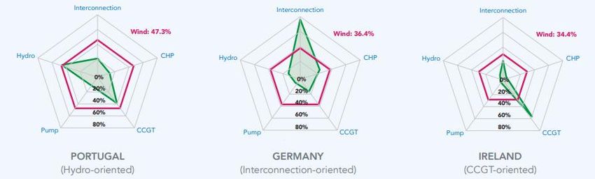
Power flow tool for active distribution grids and flexibility analysis

       Abstract

The effects of the energy transition are leading towards energy models in which
decentralized generation is a reality and a source of debate at the time of planning,
assessing the risks and optimizing its performance. One of the implications of this trend is the
need to test multiple scenarios and configurations in the environment in which the
decentralized generation is being deployed: the distribution network.

This thesis is aimed at dealing with such need by proposing a tool based on the pandapower
library (python) to offer more automation, customization and graphic capabilities during the
process of creating networks, testing different scenarios using power flow analysis and
obtaining a clear visual output via graphs and heatmaps.

It has been sought to use open source code, as python and its libraries are, not tied to any
commercial restrictions and making the tool as generic as possible. However, a comparison
against Matpower package (Matlab), endorsed with decades of use, is carried along the
thesis to provide more robustness to the output.

The tool will be able to read separate network elements’ data in a standard format (.csv) and
assembling them internally as a network, making the tool independent in terms of size. In the
same direction, it will include different menus to allow fast addition of elements or flexibility
measures providing easiness of use and saving time for the user. Finally, it will account with
heatmaps and schematic representations of the network that will help to identify common
flexibility issues such as overloaded lines or voltage deviations.

3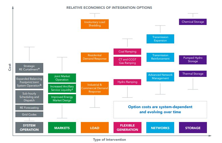
Power flow tool for active distribution grids and flexibility analysis

5
Table of contents

MASTER IN ENERGY ENGINEERING (MUEE) ........................................................................................ 1
ABSTRACT .................................................................................................................................................... 3
TABLE OF CONTENTS ................................................................................................................................ 6
1.      INTRODUCTION ................................................................................................................................. 11
     1.1.       OBJECTIVES..........................................................................................................................................12
     1.2.       SCOPE ..................................................................................................................................................12
     1.3.       STATE OF THE ART ...............................................................................................................................12
2.      COMMON ELECTRICITY POWER SYSTEM DESCRIPTION ........................................................ 15
     2.1.       BRIEFING ON ELEMENTS AND SCHEME .................................................................................................15
     2.1.1.       GENERATION ........................................................................................................................................16
     2.1.2.       DEMAND AND CONSUMPTION..................................................................................................................18
     2.1.3.       TRANSMISSION AND DISTRIBUTION ...........................................................................................................19
3.      ELECTRIC POWER SYSTEM FLEXIBILITY.................................................................................... 22
     3.1.       STORAGE ..............................................................................................................................................23
     3.2.       DEMAND-SIDE MANAGEMENT ..............................................................................................................25
     3.3.       ADDITIONAL RESERVE CAPACITY ........................................................................................................26
     3.4.       RETROFITTING OF EXISTING FACILITIES ...............................................................................................26
     3.5.       ANCILLARY SERVICES ...........................................................................................................................27
     3.6.       FLEXIBILITY IN DISTRIBUTION NETWORKS ............................................................................................28
     3.6.1.       DISTRIBUTED ENERGY RESOURCES PENETRATION IN THE MV LAYER...........................................29
4.      POWER FLOW ANALYSIS ................................................................................................................ 32
5.      SELECTED APPROACH AND ANALYSIS TOOLS ........................................................................ 37
     5.1.   PANDAPOWER ......................................................................................................................................37
     5.1.1.   ELEMENTS MODELS’ AND DESCRIPTION...........................................................................................40
     5.2.   BRIEFING ON OTHER ANALYSIS TOOLS .................................................................................................45
     5.3.   CASE COMPARISON ..............................................................................................................................47
6. TOOL PROPOSAL FOR AUTOMATION AND CUSTOMIZATION OF BASIC SCENARIO
TESTING ...................................................................................................................................................... 58
BUDGET ....................................................................................................................................................... 83
ENVIRONMENTAL IMPACT ...................................................................................................................... 84
CONCLUSIONS ........................................................................................................................................... 85
ACKNOWLEDGEMENTS ........................................................................................................................... 86
BIBLIOGRAPHY .......................................................................................................................................... 87
Power flow tool for active distribution grids and flexibility analysis
List of figures
Fig. 1: EPS overall scheme [2]. ............................................................................................................. 15
Fig. 2: a) Conventional thermal plant shceme. [10] b) General wind turbin system and control scheme.
[11] ......................................................................................................................................................... 17
Fig. 3 a,b,c: double-circuit towers of 110-150, 220-275, 400-500 kV respectively. d,e,f: single-circuit
towers in triangular, delta and horizontal formation respectiely [12]. .................................................... 19
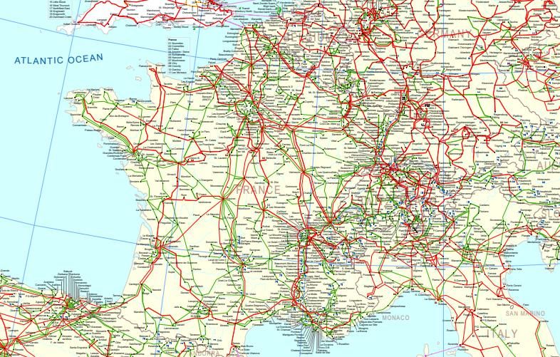
Fig. 5: European transmision system. ENTSO-E. ................................................................................. 20
Fig. 4: Example of a meshed configuration. [17] ................................................................................... 20
Fig. 6: Example of a radial configuration. [17]. ...................................................................................... 21
Fig. 7: Inherent primary (potential) source of flexibility by country with the maximum share of wind
power (red). Source: [29] Citing Yasuda, Y. 2013. “Flexibility Chart: Evaluation on Diversity of
Flexibility in Various Areas.” .................................................................................................................. 22
Fig. 8: Storage technologies by discharge capacity and discharge time. Source: [21] ......................... 23
Fig. 10: Sources of flexibility by type and cost. Source: [20]. ................................................................ 28
Fig. 10 Example network composed by 5 buses (numbers 1 to 5) with 2 generators (buses 1 and 5)
and 4 loads (buses 2, 3, 4 and 5).[11] ................................................................................................... 32
Fig. 11 Power flow initial variables briefing. Source: [20] ...................................................................... 33
Fig. 13: Addmitance mattrix shape ........................................................................................................ 35
Fig. 14: Line parameters stored in a table type structure. ..................................................................... 38
Fig. 15: Schematic example of the pandapower network stored data tables. Source: [16]. ................ 39
Fig. 16: Net dictionary containing result data from a PF. ...................................................................... 39
Fig. 17: Bus equivalent circuit Source: [17]. .......................................................................................... 40
Fig. 18: Minimal defining parameters for bus creation in pandapower. Source: [17] ............................ 41
Fig. 19: From left to right and downwards; ‘T’ model transformer, ‘Pi’ model transformer and three 2-
winding transformers in ‘wye’ connection. Source: [17] ........................................................................ 42
Fig. 20: Load as PQ bus scheme represented in pandapower. ............................................................ 43
Fig. 21: Generator as PV bus scheme. Note the phasor is pointing inversely as the injection sign is
negative. Source: [17]............................................................................................................................ 44
Fig. 22: Summary table of key features about pandapower and other tools. Source: [15]. .................. 45
Fig. 23: Matpower casefiles power flow speed comparison .................................................................. 46
Fig. 24: Case4gs briefing and bus data. ................................................................................................ 47
Fig. 25: Plot of the case4gs net using Plotly library. ............................................................................ 47
Fig. 26: Loading an included case with Pandapower. ........................................................................... 48
Fig. 27: Definition of the elements and parameters to replicate case4gs. ............................................ 48
Fig. 28: Bus and external grid results after pf........................................................................................ 49
Fig. 29: Generation and load results after pf. ........................................................................................ 49
Fig. 30: Line results after pf. .................................................................................................................. 50
Fig. 31: Expanded view of the line results dataframe. .......................................................................... 50
Fig. 32: Bus and external grid results for the inbuilt Case4gs after pf. ................................................. 52
Fig. 33: Generation and load results for the inbuilt Case4gs after pf. ................................................... 52
Fig. 34: Line results for the inbuilt Case4gs after pf. ............................................................................. 52
Fig. 35: Matpower case structure of case4gs() showing bus data. ....................................................... 55
Fig. 36: Matpower bus results data structure. ....................................................................................... 55
Fig. 37: Change of resolution to carry deviation analysis. ..................................................................... 55
Fig. 38: Matpower bus results after pf with 9 decimal positions. ........................................................... 56
Fig. 39: Matpower branch results after pf with 9 decimal positions. .................................................... 56
Fig. 40: Structure of the element creation automation. ......................................................................... 59
Fig. 41: CSV example where ‘X’ contains the parameters of the element and ‘Y’ contains each
different element of the same type. ....................................................................................................... 60
Fig. 42: Use of the net reader tool to replicate save the structure of the c4gs net. The time is recorded
at the bottom of the figure...................................................................................................................... 60
7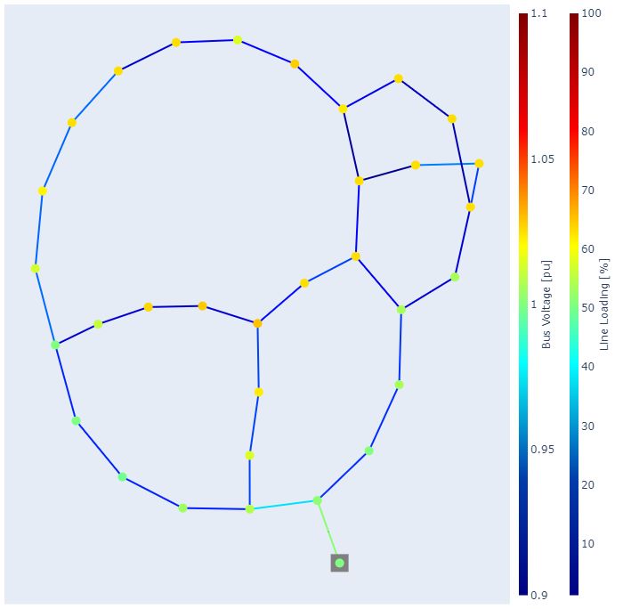
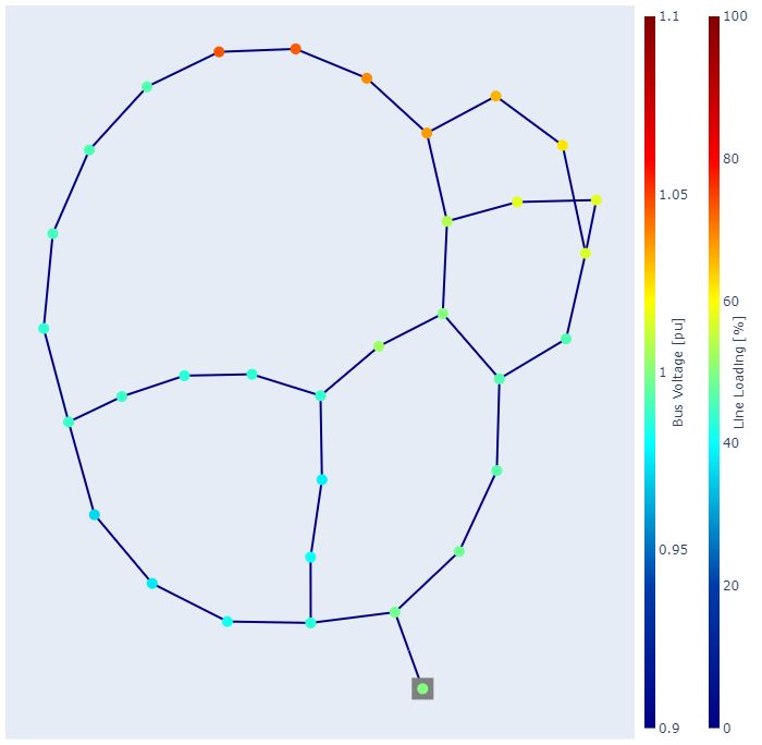
Fig. 43: Heatmap with legend showing the line loading, the losses and the power injected in evey line.
............................................................................................................................................................... 62
Fig. 44: Isolated heatmap showing the line loading (%) avoiding scale interference with other different
magnitudes. ........................................................................................................................................... 62
Fig. 45: Case 4gs network plotted with and without geocoordinates (left and right respectively). ........ 63
Fig. 46: Case IEEE 24-bus rts network plotted with and without geocoordinates (left and right
respectively). ......................................................................................................................................... 63
Fig. 47: Power flow results plotted over network scheme. .................................................................... 64
Fig. 48: Example of the menu implemented. ......................................................................................... 65
Fig. 49: IEEE-33 Network data. ............................................................................................................. 66
Fig. 50: IEEE-33 Network scheme. ....................................................................................................... 66
Fig. 51: IEEE-33 bus results power flow. .............................................................................................. 67
Fig. 52: IEEE-33 Branch/line results . ................................................................................................... 68
Fig. 53: Heatmap showing line loading percent, losses and power through line. ................................. 68
Fig. 54: Active and reactive losses of the system under nominal conditions. ....................................... 69
Fig. 55: Heatmap of bus voltage (pu) over bus index ........................................................................... 70
Fig. 56: Power flow bus results with increased scattered loads and voltage violated buses (5%
threshold). .............................................................................................................................................. 71
Fig. 57: Line results with increased scattered loads scenario. .............................................................. 72
Fig. 58: Power flow results over network scheme. ................................................................................ 72
Fig. 59: System losses (scattered increased loads scenario). .............................................................. 73
Fig. 60: Heatmap of active losses (MW) per line index. ........................................................................ 73
Fig. 61: Menu to enhance the speed at testing with shunt capacitors. ................................................. 74
Fig. 62: Power flow before applying shunt capacitors (left) and power flow after shunt capacitors have
been deployed (right) ............................................................................................................................. 75
Fig. 63: Power flow bus results after DER penetration scenario. .......................................................... 76
Fig. 64: Power flow bus results after DER penetration scenario. .......................................................... 77
Fig. 65: Heatmap showing line loading percent, losses and power through line. ................................. 78
Fig. 66: Heatmap showing line loading percent at scale. ...................................................................... 78
Fig. 67: Heatmap showing active power losses at scale. ...................................................................... 78
Fig. 68: Power flow results over topological shceme showing the overloading in line 0. ...................... 79
Fig. 69: Menu implemented for automatic allocation of storage systems. ........................................... 80
Fig. 70: Heatmap showing net status after placing 5 MW storage systems. ........................................ 80
Fig. 71: Power flow results over topological shceme showing restored lines overload after storage
deployment. ........................................................................................................................................... 81
Fig. 72: Line losses with adapted scale. ................................................................................................ 81
Power flow tool for active distribution grids and flexibility analysis

          List of tables

Table 1: : Briefing with some of the storage technologies’ characteristics. Source: [21] ...................... 24
Table 2: Average execution time of the case4gs from scratch. ............................................................ 51
Table 3: Average execution time of the inbuilt case4gs. ....................................................................... 53
Table 4: Bus results deviation. .............................................................................................................. 53
Table 5: Ext. grid results deviation. ....................................................................................................... 54
Table 6: Line results deviation. .............................................................................................................. 54
Table 7: Results’ relative deviation. ....................................................................................................... 54
Table 8: Average execution time of the inbuilt case4gs. ....................................................................... 56
Table 9: Bus and generation results deviation (Matpower vs Pandapower). ........................................ 57
Table 10: Branch results defiavion (Matpower vs Pandapower). .......................................................... 57
Table 11: Time records (avg.) as nº of buses increase and efficiency.................................................. 61
Table 12: Distributed loads data. ........................................................................................................... 70
Table 13: Distributed generation data. .................................................................................................. 75
Table 14: Project associated costs. ....................................................................................................... 83

9
Power flow tool for active distribution grids and flexibility analysis

            1. Introduction

In the recent years, concerns about environmental crises, energy safety and notorious
enhancements in Information and Communication Technologies (ICT), among other reasons,
have leaded to a shift in energy policies, power systems (PS) around, as well as people’s
behavior towards markets and the way energy is being consumed [2].

While electricity represents the 20% of the total final energy consumption today, the share is
raising and, specifically, the weight of renewable energy sources (RES) generation, which in
2019 reached 9,26%1. But an even more significant fact is that, in a global scale, the RES
accounts for the 50% of the electricity generation growth [6], suggesting a deeper penetration
of that sources along the following years. That growth is also being reflected in a local scene,
where the liberalization of the energy market together with incentive policies are causing the
appearance of new actors (prosumers2) taking active roles in the power systems and thus,
implying a trend of change towards the decentralization of the actual PS [3]. The translation
of such trend can be observed in the growing presence of distributed energy resources
(DER), ranging from households with PV panels to entire fleets of electric vehicles (EV) as
well as self consumption for commercial activities (3 kW to 50 MW) injecting power in lower
layers of the power system (medium voltage). The implications of the deployment of DER are
positive, the on-site generation is more efficient and less expensive than purchasing it from
the electric utility, permits the use of multiple local storage strategies to enhance the load
profiles and contributes with environmental health due to the fact that the great majority of
the DER are composed by RES [7]. However, it carries challenges regarding flexibility in PS
to accommodate this growing input of variable renewable energy sources (VRES). Building
the assets to bring the needed adequacy and flexibility in the PS will require an update to the
market layout [3] as well as enhanced planning, network status and probabilistic analysis.

1
  Excluding hydro-power [4].
2
  A prosumer, in the energy sector, is a consumer which also embraces the role of producing, selling trading or
storing energy [5].

11
1.1. Objectives Normally, testing a system with a strong penetration of DER require sets of data that can either be provided by institutions, distribution/transmission system operators (DSO/TSOs) or data banks. This can imply large amounts of time preparing the environment and, in the event of testing multiple scenarios, limiting the number and variability of them. It seems appropriate then, to use available resources in order to provide a tool for easiness and automation in obtaining information from network status in different scenarios, assessing the impact of the implemented measures and using graphic resources available to shed light to the results. Thus, the objectives of this thesis are the use of open source code (availability) to concoct a tool that must be able to automatically read and process data to build a network testing environment (automation in setting up). In addition, it has to be able to easily modify the current network to generate different scenarios with ease (customization and automation in testing) and perform power flow analysis as an output. Finally, it should include graphic support to allow a better visualization of the results of the power flows aimed to draw basic conclusions about flexibility issues that the different scenarios might bring. To summarize, the tool must be a basic instrument that helps shortcutting, in terms of time and work the path from ‘obtaining data from a network’ to ‘providing basic results about status and flexibility of current scenarios’. 1.2. Scope The scope of the project is centered in providing an easy-to-use ground that can be scalable and customizable beyond this thesis to provide the desired output by the user. It is out of the scope everything related with the implementation of advanced analysis algorithms or topology/planning optimization, which still can be implemented afterwards as a next steps recommendation outside this thesis. 1.3. State of the art There’s a vast amount of sources about the introductory topics discussed in this thesis: energy transition, role of DER, flexibility and resilience [5], [6], [7], [9], [16] among others. All of them coincide in the idoneity of the new models regarding enhanced efficiency, cleaner sources of energy and the decentralization of the energy systems in many spheres (market,
Power flow tool for active distribution grids and flexibility analysis

competition, and scattered generation).

Also, they put special emphasis in the impact of the new trends towards the energy price and
the redesign of the power systems to accommodate the growing numbers of VRES (smart
grids, FACTS, storage).

There are other sources that treat specific parts of the introductory topics, such as the
optimal operation of networks with strong penetration of DER, control architecture of the
future power systems or optimal planning for the distributed resources [10], [15], [17], [19],
[26]. Those sources develop either algorithms to allocate the specific amount of supply at the
required buses to achieve optimal grid performance or also analyze possible control solutions
for incoming challenges in power flexibility. They coincide in suggesting that there are areas
in which real implementations of control strategies and experimentation are being made, as
would be the case of California, Denmark and northern Europe to cite some, but there will
still be needed a strong investment in ICTs in order to deploy such strategies (investments
already in process in many EU countries regarding digital meters for end-users and sensors
along the power lines).

The main part of the sources working on simulations use the inbuilt test feeder cases from
IEEE (e.g. 14-bus system, 30-bus system) on their respective software to perform their
analysis and tests but just few talk about ways to read further input data from different
networks or how to accommodate multiple tests with ease without a linear relation between
size and time.

13
Power flow tool for active distribution grids and flexibility analysis

           2. Common electricity power system description

To provide such a commodity as it is the electric energy to the end user requires of a set of
conditions and physical aspects that ensure a reliable, uninterrupted and safe supply. Those
determining factors are specific enough not to leave much leeway far from the standards in
terms of structure and configuration. This section intends to be a briefing about the
mentioned standards and a general depiction of the elements conforming the structure of the
electric power system as they are seen nowadays and worldwide.

     2.1. Briefing on elements and scheme

Generally, the current Electric Power Systems (EPS) are considered centralized, which mean
they rely on large production plants to supply the customers through the transmission and
distribution systems connections along the territory [1]. Therefore the structure of the power
system lays, in broad terms, upon a generation, transportation and consumption layers,
being them all interconnected and synchronized in real time.

                                    Fig. 1: EPS overall scheme [2].

15
As seen in Fig. 1, the generation plants produce an output which will be raised in voltage as
soon as it leaves the facility to be transmitted with the least possible losses. However, some
consumers will be fed directly in such High Voltage (HV) layer due to the energy intensity of
their own activities (metallurgic foundry, construction material facilities, etc) which require a
high power demand. The same happens to the Medium Voltage (MV) consumers, which are
fed at their own interest between 1 and 45 kV or, even some specific generation technologies
such as Photo Voltaic (PV) plants, wind farms or Combined Heat and Power (CHP), which
can inject their distributed power generation directly in the MV layer due to its proximity and
size [8].
The power lines of both layers (HV and MV), despite carrying the same task have different
configurations as their approach is slightly different. In one hand the HV layer’s primary task
is to transmit high amounts of power to long distances with reliability, thus meshed
configurations are chosen to reach that goal rather than radial, which are used in MV layers
to spread along the territory to reach the maximum number of users as its voltage and power
steps down across the different transformation spots. These configurations will be briefly
commented on the section “Transmission and distribution”.
2.1.1. Generation
The electricity production relies on different kind of centers that include classic (conventional)
power plants which transform primary sources such as coal, gas, nuclear fuel or residues into
electric energy via thermodynamic cycles involving steam or/and gas turbines. Along with the
classic or traditional technologies we found a range of renewable or cleaner stations, in
growing pressence in the power systems around, which rely on renewable sources such as
sunbeams, wind, geothermic energy or tidal energy among others to provide the electricity
supply. Both of them, conventional and renewable power stations must provide its electric
output in a very specific magnitudes of waveform (sinusoidal), three-phase signal with
standarized frequency and amplitude (which have to be controllable) [8].
Generally, the conventional power plants which produce a large thermal inertia on their
boilers, reactors or turbine exhausts have longer times of readiness and cannot be
disconnected and reconnected with ease for demand matching purposes [16]. They rely on
primary, secondary and tertiary control blocks which allow different time responses to
demand variations, nonetheless with scale limitations (e.g. a combined cycle power plant
with 3 turbines of 100 MW each will not be able to produce 112 MW sustained, but 40 to 102Power flow tool for active distribution grids and flexibility analysis
MW x 3 approximately).
The layout of a conventional thermal plant (the common part Fig. 2) is generally formed by a
boiler or heat source, the piping network, the pumping system, the steam or/and gas cycle
(containing the turbine stage and the condenser) and, finally, the generator.
Fig. 2: a) Conventional thermal plant shceme. [10] b) General wind turbin system and control scheme. [11]
The main differences will rely on the heat source, be it coal, nuclear energy, gas-fired or even
solar concentration technologies, which accounts for renewable sources but, in essence,
share the same thermodynamic cycle and elements. On the other hand, the hydro
technologies are classified also as conventional but rely on water turbines which take
advantage of the head3 of rivers and dams to transform the energy of the water flow into
mechanical energy and electrical output at the generator terminals [8].
In the renewable technologies side, the layouts can vary notably due to the fact that there are
plants using thermal cycles, others relying on photochemical processes, potential energy and
so on. Mainly, from wind farms to photovoltaic installations, all of them usually count with a
3
Water pressure under the column of fluid. Expressed in length units.
17strong presence of converters, filters and power electronics in general, aimed to
accommodate either the variable nature of the sources they use or the electric output in DC
which would be the case of photovoltaic stations. The range of power scalability in renewable
sources is higher due to both, the composition of the systems itself in smaller generators
(e.g. wind farm composed by fifty 3 MW wind turbines, photovoltaic station with 400 panels of
300 W each) and the multiple strategies that allow to regulate power output (apart from the
integrated power electronics) such as tilt angle modification of wind turbines, 2-axis tracking
in the case of solar PV or solar thermal and flow regulation in geothermal facilities [10].
2.1.2. Demand and consumption
The ultimate aim of the power system is supplying the end-user with, as mentioned before, a
reliable, uninterrupted and quality service. In contrast to generation, the demand is
distributed along the territory and the users can be of multiple kinds and requirements. As
shown in fig. 1, there are consumers ‘pinned’ in different subsectors of the transmission layer
according to their needs. For instance, an intensive metallurgic factory will need of a greater
demand of power to feed their arc furnaces than a common household, therefore, the factory
transformers will be directly connected to a substation from the distribution or even
transmission layer (e.g. 132 kV busbar) [8].
Loads such as the above commented metallurgic factory produce serious disturbances to the
power quality and demand variation like flickers4, which are hard to be controlled for being
attributable to the side of the consumer. Despite this, in general terms the demand curves
are able to be solidly forecasted due to the fact that the main parts of the curves take fixed
patterns over time. Normally, showing an offset minimum value during low demand periods
which raises in value and variability around the peaks when the consumption is higher and
there are more services active and thus, more uncertainty (statistically).
The power quality requirement has also to be continuously addressed as many widely used
appliances like computery, televisions or any other utilities which need for a certain power
stability to work correctly. Aside from flickers, other power quality issues that are dealt with
(more emphatically in the developed countries) are supply outages which are interruptions in
the power supply, overvoltages which are surges that can damage and even burn
equipments and can be caused by lightnings, voltage drops that can be caused by faults or
4
Fluctuations in the voltage amplitude.Power flow tool for active distribution grids and flexibility analysis
peak load startups (specially rotating machines demanding an overconsumption when
starting), voltage harmonics which are deviations from the fundamental frequency of the
voltage wave, and so on.
2.1.3. Transmission and distribution
To interconnect the production power stations with the consumption clusters there are two
main layers, one devoted to long the distance transportation (transmission), which can be
identified by the higher voltage levels, as well as the wire sizes and configuration; and
another layer aimed to spread around the territory, normally in radial configurations to reach
and feed the end users.
a) b) c)
d) e) f)
Fig. 1 a,b,c: double-circuit towers of 110-150, 220-275, 400-500 kV respectively. d,e,f:
single-circuit towers in triangular, delta and horizontal formation respectiely [12].
As commented above, the voltage levels of the transmission system are higher to cross
greater distances with fewer losses, such voltage levels would be in a range within 800 kV to
132 kV, being 220, 400 and 500 kV common standards for transmission voltages. The HV
lines are usually configured in meshed layouts to provide more than one path to the energy
flow in case of service interruption or other maintenance issues. The dominant type of
transport medium in such lines is overhead wires attached to towers with different
19configurations (fig. 3). Typical line parameters such as inductance strongly depend on these
relative geometric positions of the three phases on the tower. Even though underground lines
in HV voltages can be found nearby some city areas they are scarce, as the price of the
insulation needed due to its proximity to the ground is very high in comparison to overhead
configurations [6].
Fig. 2: Example of a meshed configuration. [17]
The transmission lines are commissioned to reach the distribution or subtransmission
substations, which will decrease its voltage in the transformation nodes to feed the
distribution networks. Alongside transformation tasks, the substations carry out
measurements, protection and interruptions of the line, all of them necessary to synchronize
different activities like isolation of an area due to blackout, maintenance tasks, disconnection
operations among others.
Fig. 5: European transmision system. ENTSO-E.Power flow tool for active distribution grids and flexibility analysis
The distribution grids are, as mentioned above, devoted to ‘spread’ the power transmitted by
the HV lines over the different consumers around. There’s normally a ‘frontier’ layer between
distribution and transmission (still accounted as the lower part of transmission grid) which still
operates in quite high voltages, from 45 to 132 kV (depending on the country) and its mission
is to step down the voltage to the nominal MV distribution values, which are for instance 20,
15 or 6.6 kV[8]. Such ‘frontier’ still operates partially in a meshed structure or with an open
loop configuration. When it reaches the mentioned reduction substations (MV and LV levels)
the structure and operation becomes, in broad terms, radial (Fig. 6).
Fig. 3: Example of a radial configuration. [17].
The voltage reduction reasons are the safety for the end-users as well as the reduction of the
insulation requirements in the electric appliances [16]. Such voltages are standardized by the
IEC600385, which states that the MV for three-phase systems are 3.3, 6.6, 11, 22, 33 kV,
within the 1-35 kV margin.
The radial networks structure commonly used in distribution grids have simple and cheap
topologies with easy implementations of voltage compensation techniques. The distribution
system operator (DSO) must ensure the security and reliable operation requirements. a with
the drawback of disconnection of all lines in case a upstream line or node fails.
5
International Electrotechnical Comission.
213. Electric Power System flexibility In order to tackle with the instabilities and uncertainties entailed with Variable Renovable Energy Resources (VREs), there is a range of options which enhances the flexibility of the systems and subsystems involved. Such strategies can be classified according to the layers in which they are operating or the economic suitability according to technical and market variables. In this work, the assessment will be focused in technical reasons and of feasibility. In the actual power systems worldwide there is an inherent level of flexibility composed by the already existing control techniques to adjust an already uncertain demand of supply; which can consist of short dispatch time power plants, spinning inertial blocks among others. Fig. 4: Inherent primary (potential) source of flexibility by country with the maximum share of wind power (red). Source: [28] Citing Yasuda, Y. 2013. “Flexibility Chart: Evaluation on Diversity of Flexibility in Various Areas.” An example of such variability across systems can be seen in Fig. 7, where the red pentagon depicts the maximum share of wind power in an hour of relative demand (data prior to 2013) and the area highlighted in green shows the installed capacity of potential flexibility sources. However, as there still are external factors that can impact on these sources such as market variables, in the case of interconnection-oriented systems, or capacity issues regarding hydro-pumped, as well as issues in the gas supply in the case of CCG; there’s not a direct translation into the reality and that’s why they are still ‘potential’ sources in this kind of diagrams. Following this chapter, ways of flexibility enhancing in power systems will be listed and briefly discussed.
Power flow tool for active distribution grids and flexibility analysis

     3.1. Storage

One of the most well known, stable and deployed source of flexibility. Storage systems
provide a wide range of discharge rates, capacities and times of response which allow them
to adapt quickly and durably to unpredicted load changes (when mixed and deployed
efficiently). In the event of excess renewable generation and/or during low-demand periods,
energy can be stored through pumped hydro, compressed air (CAES) or in electrochemical
batteries to cite a few of them. In the same way, in the event of low share of
cheap/renewable sources they can dump in the grid their stored energy to provide a cost-
effective and environmentally friendly solution [21].

             Fig. 8: Storage technologies by discharge capacity and discharge time. Source: [21]

Although some of the listed technologies are mature, there are still many of them in early
stages of development (superconducting technologies, advanced chemical storage) and
some others carry with expensive variables which brake an efficient and wide deployment. In
the same direction, pumped hydro or CAES present difficulties at choosing suitable locations
to be deployed as well as issues regarding the environment, due to its harsh impact on a
wide area.

23
In the recent times, research on an efficient combination (and layering) of storage
technologies has been made to reduce costs and apply optimal time-capacity response in
the distribution and transmission networks. Deploying large scale technologies in the HV
layers and distributed smaller facilities with faster response in the MV side has proven to
increase the system flexibility.
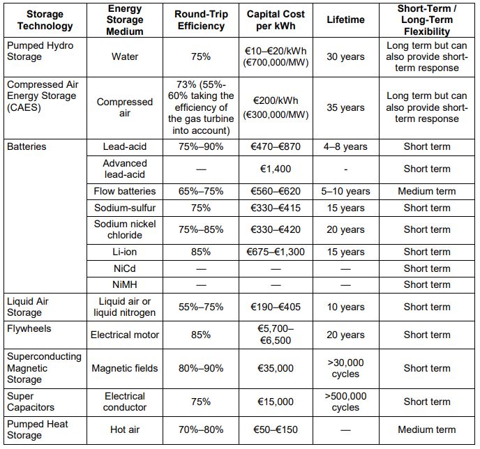
Sizing the appropriate storage system output and capacity ends up with the assessment
within a set of different technologies and allocated costs (€/kW, €/kWh). In the next Table 1,
basic technical and associated cost characteristics are attached.
Table 1: : Briefing with some of the storage technologies’ characteristics. Source: [21]
The usually high capital cost of storage facilities makes it challenging to deploy certain
amounts of it without the appropriate policies. Furthermore, some of the benefits provided by
the energy storage systems can also be reached by other measures such as Demand-Side
Management (DSM) or additional reserve capacity, making it necessary to compare it withPower flow tool for active distribution grids and flexibility analysis
other options before its implementation.
3.2. Demand-Side Management
The range of mechanisms devoted to intervene and partially change the magnitude of the
end-user electricity consumption profiles as a mean of enhancing network flexibility is
baptized as Demand Side Management (DSM) [23]. Mainly, it can be splitted into three
different categories depending on whether they are reducing, increasing or rescheduling the
energy demand.
The primary source of flexibility among the three types, should be the rescheduling (load
shifting) preferably, which in contrast with the others don’t necessarily compromise any final
product/service nor its continuity due to lack or excess of energy (switchable loads with less
than 100% utilization rate). Otherwise, DSM with load shifting may need indirect ways of
storing energy, using for example building heating/cooling inertias, rotating machines such as
milling machines or washing lines which can swap timetables, and so on.
DSM proves to be useful in the timescale of the VREs variability disturbances (1-12h) as well
as playing an important role in the deployment of energy efficiency through the
implementation of control and measurement equipments in households and secondary
sector levels [23]. This paves the way to a more active role in the market by the consumers
and can help reducing the use of power in peak periods as well as reducing the average spot
price of energy.
Many field studies and surveys have reported positive results about the potential of DSM
measures, either implemented via policies and market mechanisms or via load control
(requiring a still incipient ICT deployment). Such studies shown, as an example, a 13-16% of
peak-hours consumption reduction in Finland during a dynamic pricing test (4:1 peak-to-
normal price ratio) or 25-28% using a 12:1 ratio [33]. On average, according to P.D. Lund et
al., studies on VRE-DSM joint strategies report a 20% cost reduction and a increase of 10-
20% VREs consumption.
253.3. Additional Reserve Capacity Any EPS relies on a certain amount of extra capacity (contracted by the system operators) which contributes on system stability by switching those reserve generators when needed. The sizing problem hadn’t been a major issue since is quite simple to determine a nearly optimal amount of reserve by establishing boundaries of probability that state improvable or very rare a cascade of events in which such reserve is surpassed. But since then, the penetration of VREs has been increasing over time and the need to expand the additional reserve capacity has been widely discussed. According to NREL 2011, as the EPS around the world consist of different resources available and characteristics for instance the frequency response or the transmission network, every TSO/DSO may operate with the risk in a different way, providing schemes adapted to their reality and thus, with different definitions for categories and capacity required. This will translate into in a mix of additional reserves capable of response in any timescale and in accordance with the environment. However it is interesting to point the conclusions drawn from NREL 2011 comprehensive review on VREs impact on operating reserves in the US and Europe, cited by [21]. To summarize, the study concludes that no additional contingency reserves were required, in the timescale of instantaneous response, because the unpredictability of the VREs acts in a distinct time frame of such reserves. On the contrary, the needs as the penetration of VREs increases in the systems of the study were focused on the regulating, following and ramping reserves dominion (but never reaching a 1:1 ratio). Concretely, the average increase in the ‘mix’ of reserves (load following, ramping, etc) never exceeded the 15% of the newly installed VRE capacity (of wind power in that case). 3.4. Retrofitting of existing facilities Other options explored in studies regarding US coal sector provide examples of successfully retrofitting existing CPP to expand their performance limits and regulations which ends up translating into an enhanced flexibility of facilities initially devoted as a base generation (or inflexible). The results speak by themselves, showing a reduction of the minimum power output into less than 20% of the nameplate capacity (in that case, due to the big inertia of the thermal cycles they are suitable to be operable in load-following mode).
Power flow tool for active distribution grids and flexibility analysis

In the same way of flexible generation but in a smaller scale, the use of distributed combined
heat and power facilities are proven to be a source of flexibility by adapting their output
between heat and electric energy on benefit for demand matching needs. Apart from that, the
isolated efficiency of those systems increase with both the heat recycling usage and the way
the indirect thermal energy storage can be used to favor the flexibility as commented in
section 3.1.

     3.5. Ancillary services

The ancillary services are rather a category that comprises previous mentioned flexibility
sources than a specific measure applied to a specific time frame. Despite that, this chapter
will mainly emphasize the ‘fast response’ ancillary services such as voltage support,
frequency response, balancing services, inertial response and so on.

In the timescale from milliseconds to minutes, the power quality standards require the use of
voltage control (reactive power) and frequency (active power) to adjust the fluctuations
caused by a range of causes (wind, solar outputs deviations among others). In that time
frame, also de DSM can enter in action in the frequency stability efforts, specially the rotating
loads which provide inertia in the same way as a conventional generator. Together with that,
fast response storage technologies with small capacities but high discharge ratios such as
supercapacitors, superconducting magnets, and flywheels also play an important role over
fast-ramping power disturbances[23].

In a slightly extended timescale (from minutes to one hour), we can find the online spinning
and contingency reserves, that consist on the generator capacity connected at any time with
capacity to both ramp up in short timescales as well as mid-term functioning (typically
between 30 to 60 minutes) before the reserve generators and facilities can start normal
operation after a major failure have occurred. In the same way, the DSM again can play a
significant role by using shiftable loads for short times before the other systems can start
ramping up.

27
Among the mentioned ancillary services, there is also the load leveling mode which displaces
the load from valley to peak hours and the algorithms that intervene directly in switches and
load tap changers (LTCs) 0. The load leveling can be achieved through Compressed Air
Energy Storage (CAES) or pumped-hydro which can decrease the need of peaking power
plants operating during high demand periods.
Fig. 10: Sources of flexibility by type and cost. Source: [20].
To summarize, in Fig. 10 there is a briefing with the different flexibility areas of intervention
and their cost in relative terms.
3.6. Flexibility in distribution networks
The MV layer or distribution layer is the subsystem where the trend of renewable and
Distributed Energy Resources (DER) injection is increasingly taking place during the last
decade, due to a wide range of reasons regarding incentive policies, climate concerns and
market opportunities. This fact makes interesting the creation of a tool which can make it
easier to perform the basic analysis of multiple distribution network configurations and
scenarios involving renewable power injection without the need of continuously redesigningPower flow tool for active distribution grids and flexibility analysis
from scratch the whole network or test.
The reasons why such injection of DER will take place in MV levels are tied to the size itself
of the generation, which can vary from medium or small sized plants powering entire areas to
prosumers or selfconsumers at a household level, which will inject from the lowest layer of
the network. Apart from that, other advantages like the losses reduction in transmission (due
to smaller distances) as well as generation make it worthy to inject at such levels. That’s why
the treated environment in the project will be the MV layer and thus it will be slightly more
detailed in the next section.
3.6.1. Distributed Energy Resources penetration in the MV layer
The normal trend of the actual traditional energy system is to become more decentralized
mainly in terms of generation. This fact cause, among other issues, a higher probability to
find mismatches and congestions between demand and supply due to the hosting of an
increased presence of VREs, forcing the DSOs to cope with such instabilities.
Those challenges (of hosting DER/VREs in greater ratios) can be listed as follows:
- Thermal ratings
- Voltage regulation
- Reverse power flows
- Rapid voltage change
- Islanding
- Protection
- Power quality
Thermal ratings
As DER can change the current flows, it can affect the maximum amount of electrical current
that is permitted in a line (thermal rating), overheating it or violating the safety requirements.
Possible (and oversimplified) solutions: Enhance storage capacity, addition of supercaps, EV
fleet with bidirectional connection to smooth the peak generation vs low load demand.
29Voltage regulation Fault level The need for devices to adjust the line voltage (OLTC) increases the more decentralized and bidirectional the power flows are, with its consequent increase in investment and OPEX. That’s why expanding the capability of the voltage regulation in the MV network can substantially increase the overall costs. Fault level The interconnection of the DER are contributors to the fault current magnitude and thus, the designed short circuit capacity of the MV grid can be exceeded if the initial design hadn’t taken into account the addition of DER at some point. Reverse power flows Related with the voltage regulation point, a reverse power flow applied on the mentioned OTLCs can cause problems on their normal operation. Islanding One of the capabilities of a distribution grid with high presence of DER is the ability to work in islanded mode, which means that is able to supply its own loads with its own generators without relying temporary (can vary) on the main grid. The issue here is to implement protocols to effectively and quickly detect when this is happening or about to happen and be able to readapt its energy output not to energize that specific area. Protection More expenditure in protections for line to ground faults in order to prevent he over voltages when the breaker trips in such scenario. In the same direction, when power exceeds demand in the distribution layer, in backfires to the transmission system. Thus, in case of ungrounded transmission system it will be needed a zero sequence relay to protect the substation transformer.
Power flow tool for active distribution grids and flexibility analysis

Power quality

Due to the already mentioned VREs uncertain nature, among other drawbacks, there’s a
range of issues related to the power quality caused. Voltage fluctuations, flicker, harmonics
among others. Not tackling with them would be translated in the possible damaging of
appliances as well as malfunctioning of electronic equipment.

31
4. Power flow analysis

When projecting or planning the performance of a determined electric network as well as
assessing expansions of the grid, there are analysis methods that allow obtaining useful
information such as losses, lines loading, reactive power flows among others, that be the
case of the power flow analysis.

                    Fig. 10 Example network composed by 5 buses (numbers 1 to 5) with 2
                         generators (buses 1 and 5) and 4 loads (buses 2, 3, 4 and 5).[11]

Given an electric network, the power flow analysis target is to determine the power to be
transmitted from every generation unit to every charge or demand point given some defined
constrictions. In addition, it also provides the resulting voltage in every network node, the
active power in every element of the network, the reactive power in every element of the
network, the aforementioned generation to be produced in each unit, the performance of the
network and overcharges or contingencies produced.

This information is necessary for studies of security, planning or stability. As a result, some
assumptions related to the real environment where the network operates have to be taken
into account:

  I.    Every network element has boundaries and limits to the power they can generate or
        transmit.
  II.   The voltage in the network nodes have to be kept in a certain ranges, to grant safe
        and reliable operation.
 III.   Any power demand can be satisfied by any combination of generation points, giving
        an infinite number of possible combinations.
Power flow tool for active distribution grids and flexibility analysis
After considering those assumptions, the full analysis can be divided into 3 main parts: The
mathematical model formulation, describing the relation between voltages and power in the
grid; the resolution of the node voltages involving numeric calculations; finally the power flow
and the load share between generator units.
The working variables can be classified as follows in Fig. 12, and the differences between
PV,PQ and Slack buses will be detailed as well as the variables coupled with every kind of
bus.
The buses can be classified as PV, PQ or Slack depending on whether there’s generation of
power or not in a bus itself. In the PV buses there is generation and thus, the active power is
known. In this kind of buses it is common to control the voltage using reactive power
regulation for that reason both power and voltage are known and reactive power to generate
is the unknown value.
The PQ buses or load buses are buses without power generation. As the active and reactive
power demand are known variables for every bus but and, in this case, the tension and the
angle are missing or unknown, they are called PQ buses.
Finally the Slack bus is used as a reference to set the phase angle magnitudes of the rest of
the buses, as the angle in each bus is found by difference. Consequently in the Slack bus
δ=0 and also as a reference bus it is useful to set it in a node where the tension will be
controllable, so the module and arguments of the voltage are known being the active and
reactive power the only unknowns left [13].
Bus Voltage Real power Reactive power
type
Magnitude Angle Gen. Load Net (Pi) Gen. Load Net (Pi)
Slack Known Known Unk. Known Unk. Unk. Known Unk.
PV Known Unk. Known Known Known Unk. Known Unk.
PQ Unk. Unk. Known Known Known Known Known Known
Fig. 11 Power flow initial variables briefing. Source: [20]
33You can also read