STATIC CODE FEATURES FOR A MACHINE LEARNING BASED INSPECTION - AN APPROACH FOR C HANNES TRIBUS - DIVA PORTAL
←
→
Page content transcription
If your browser does not render page correctly, please read the page content below
Master Thesis
 Software Engineering
 Thesis no: MSE-2010-16
 05 2010

   Static Code Features for a
Machine Learning based Inspection
                            An approach for C

                                   Hannes Tribus

School of Engineering
Blekinge Institute of Technology
Box 520
SE - 372 25 Ronneby
Sweden
This thesis is submitted to the School of Engineering at Blekinge Institute of Technology
in partial fulfillment of the requirements for the degree of Master of Science in Software
Engineering. The thesis is equivalent to 20 weeks of full time studies.

Contact Information:
Author(s):
Hannes Tribus 820919-P496
E-mail: hatr09@student.bth.se

University advisor(s):
Dr. Stefan Axelsson
School of Engineering

School of Engineering
Blekinge Institute of Technology               Internet : www.bth.se/tek
Box 520                                        Phone    : +46 457 38 50 00
SE - 372 25 Ronneby                            Fax      : +46 457 271 25
Sweden

Abstract

Delivering fault free code is the clear goal of each devel-
oper, however the best method to achieve this aim is still
an open question. Despite that several approaches have
been proposed in literature there exists no overall best way.
One possible solution proposed recently is to combine static
source code analysis with the discipline of machine learn-
ing. An approach in this direction has been defined within
this work, implemented as a prototype and validated subse-
quently. It shows a possible translation of a piece of source
code into a machine learning algorithm’s input and further-
more its suitability for the task of fault detection. In the
context of the present work two prototypes have been de-
veloped to show the feasibility of the presented idea. The
output they generated on open source projects has been
collected and used to train and rank various machine learn-
ing classifiers in terms of accuracy, false positive and false
negative rates. The best among them have subsequently
been validated again on an open source project. Out of the
first study at least 6 classifiers including “MultiLayerPer-
ceptron”, “Ibk” and “ADABoost” on a “BFTree” could
convince. All except the latter, which failed completely,
could be validated in the second study. Despite that the it
is only a prototype, it shows the suitability of some machine
learning algorithms for static source code analysis.

Keywords: static source code analysis, machine learning,
feature selection, fault detection
List of Figures

3.1   Weka Explorer     . . . . . . . . . . . . . . . . . . . . . . . . . . . .                                    9

5.1   CMore: Abstract Execution Flow . . . . . . . . . . . . . . . . . .                                          16
5.2   Holmes: Abstract Execution Flow . . . . . . . . . . . . . . . . . .                                         19
5.3   Method . . . . . . . . . . . . . . . . . . . . . . . . . . . . . . . .                                      20

6.1   Accuracy (Full) . . . . . . . . . . . .     .   .   .   .   .   .   .   .   .   .   .   .   .   .   .   .   25
6.2   Accuracy (Reduced) . . . . . . . . .        .   .   .   .   .   .   .   .   .   .   .   .   .   .   .   .   25
6.3   Average Accuracy per Category . . .         .   .   .   .   .   .   .   .   .   .   .   .   .   .   .   .   26
6.4   False Positive (Full) . . . . . . . . . .   .   .   .   .   .   .   .   .   .   .   .   .   .   .   .   .   27
6.5   False Positive (Reduced) . . . . . . .      .   .   .   .   .   .   .   .   .   .   .   .   .   .   .   .   27
6.6   Average False Positive per Category .       .   .   .   .   .   .   .   .   .   .   .   .   .   .   .   .   27
6.7   False Negative (Full) . . . . . . . . .     .   .   .   .   .   .   .   .   .   .   .   .   .   .   .   .   28
6.8   False Negative (Reduced) . . . . . . .      .   .   .   .   .   .   .   .   .   .   .   .   .   .   .   .   28
6.9   Average False Negative per Category         .   .   .   .   .   .   .   .   .   .   .   .   .   .   .   .   28

                                       ii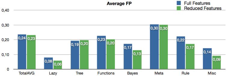
List of Tables

3.1   Data Type Range . . . . . . . . . . . . . . . . . . . . . . . . . . .    8

6.1   Paired T-Test on “Accuracy” . . . . . . . . . . . . . . . . . . . .     29
6.2   Results from WEKA for the test experiment . . . . . . . . . . . .       30

A.1 Results from WEKA for all tested machine learners . . . . . . . .         39

B.1 Results of Most Suitable Machine Learners . . . . . . . . . . . . .       40
B.2 Performance of the Classifiers on the Test Set . . . . . . . . . . .      41

                                     iii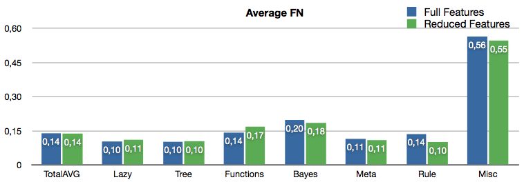
Contents

Abstract                                                                                                                     i

1 Introduction                                                                                                               1

2 Related Works                                                                                                             3
  2.1 Fault Prediction . . . . . . . . . . . . . . . . . . . . . . . . . . . .                                              3
  2.2 Fault Detection . . . . . . . . . . . . . . . . . . . . . . . . . . . .                                               4

3 Background                                                                                                                 5
  3.1 Static Source Code Analysis . . . . . . . . . . .                             .   .   .   .   .   .   .   .   .   .    5
  3.2 Types of Faults . . . . . . . . . . . . . . . . . .                           .   .   .   .   .   .   .   .   .   .    6
      3.2.1 Buffer Overflows . . . . . . . . . . . . .                               .   .   .   .   .   .   .   .   .   .    6
      3.2.2 Memory Handling . . . . . . . . . . . . .                               .   .   .   .   .   .   .   .   .   .    6
      3.2.3 De-referencing a Nullpointer . . . . . . .                              .   .   .   .   .   .   .   .   .   .    7
      3.2.4 Control Flow . . . . . . . . . . . . . . .                              .   .   .   .   .   .   .   .   .   .    7
      3.2.5 Signed to Unsigned Conversion . . . . .                                 .   .   .   .   .   .   .   .   .   .    8
  3.3 WEKA - Machine Learning . . . . . . . . . . .                                 .   .   .   .   .   .   .   .   .   .    8
      3.3.1 Machine Learning Algorithms . . . . . .                                 .   .   .   .   .   .   .   .   .   .   10
      3.3.2 Attribute Relation File Format (ARFF)                                   .   .   .   .   .   .   .   .   .   .   12

4 Problem Description                                                                                                       13

5 Proposed Solution                                                                                                         15
  5.1 CMore . . . . . . . . . . . .    .    .   .   .   .   .   .   .   .   .   .   .   .   .   .   .   .   .   .   .   .   15
  5.2 Holmes . . . . . . . . . . . .   .    .   .   .   .   .   .   .   .   .   .   .   .   .   .   .   .   .   .   .   .   18
  5.3 Methodology . . . . . . . .      .    .   .   .   .   .   .   .   .   .   .   .   .   .   .   .   .   .   .   .   .   20
      5.3.1 Experimental Design        .    .   .   .   .   .   .   .   .   .   .   .   .   .   .   .   .   .   .   .   .   21

6 Results and Analysis                                                                                                      23
  6.1 Open Source Projects . . . .     .    .   .   .   .   .   .   .   .   .   .   .   .   .   .   .   .   .   .   .   .   23
  6.2 Suitability Analysis Results     .    .   .   .   .   .   .   .   .   .   .   .   .   .   .   .   .   .   .   .   .   24
      6.2.1 Accuracy . . . . . .       .    .   .   .   .   .   .   .   .   .   .   .   .   .   .   .   .   .   .   .   .   25
      6.2.2 False Positive Rate .      .    .   .   .   .   .   .   .   .   .   .   .   .   .   .   .   .   .   .   .   .   26
      6.2.3 False Negative Rate .      .    .   .   .   .   .   .   .   .   .   .   .   .   .   .   .   .   .   .   .   .   27

                                           iv
6.2.4 Statistical Significance . . . . . . . . . . . . . . . . . . . . 29
6.3 Project Evaluation Results . . . . . . . . . . . . . . . . . . . . . . 29
7 Limitations and Validity 32
7.1 Limitations . . . . . . . . . . . . . . . . . . . . . . . . . . . . . . 32
7.2 Threats to Internal Validity . . . . . . . . . . . . . . . . . . . . . 33
7.3 Threats to External Validity . . . . . . . . . . . . . . . . . . . . . 33
8 Future Works 34
9 Conclusion 36
A Experiment Results 38
B Comparison Results 40
B.1 Complementary Results . . . . . . . . . . . . . . . . . . . . . . . 40
B.2 Conclusions . . . . . . . . . . . . . . . . . . . . . . . . . . . . . . 41
C Systematic Literature Review 43
References 51
Glossary 54
vChapter 1
Introduction
“It has been just so in all my inventions. The first step is an intuition and comes
with a burst, then difficulties arise. This thing that gives out and then that
’Bugs’ as such little faults and difficulties are called show themselves and months
of anxious watching, study and labor are requisite before commercial success - or
failure - is certainly reached.”[29] (Thomas Alva Edison in a letter to Theodore
Puskas (18 Nov. 1878))
Despite that Edison’s citation is related to his invention of a storage battery, it
reflects pretty well the situation faced nowadays by a developer or a development
team when it comes to the lengthily and often annoying process of discovering
faulty statements within a piece of software. Computer scientists mostly agree
that it will never be possible to deliver bug-free software [15], nevertheless it is
important that developers aim for reaching that state, or as it is not reachable at
all, come as close as possible by removing most of the faulty statements.
During the history of the development of software several different approaches
have been proposed with more or less acceptable results. The range of them start
from simple coding rules which focus on not introducing faults, over manual
inspection or testing up to more sophisticated ways like tool supported error
prediction or detection. Nowadays the latter gain more and more importance
as they have the possibility of simplifying the work of the developer by pointing
them to the places in the source code where the actual fault is supposed to be.
Depending on how well these tools have been developed, they are able to find
more or less complicated faults.
The quality gain achieved by using such tools can be the crucial factor for
buying one software solution instead of a competing one, and of course the sales
figures are the main driving factor for every company. Despite that the driver
seems to be clear, the question about the best possible method to find faults in
source code has no unique answer yet. Recently scientists start to think about
having some sort of intelligent, teachable system, that is not only able to detect
faults but to learn from the errors made in previous reasoning to improve its
precision in future ones.
The algorithms that can perform such a task can be summarized as machine
learning algorithms and exist already implemented and ready to use in some open
1Chapter 1. Introduction 2
source and commercial products. The difficulty in here, and the crucial problem
when it comes to combine source code analysis with machine learning is that those
algorithms are not intended to work on source code, but on instances. Therefore
the problem is how a piece of code can be translated into one or more instances
which can then be fed into such a learning algorithm.
The goals of this project are the development of a feature selection model for
a representative procedural language (it will be the C programming language for
this work) and the implementation of an appropriate parser as preprocessing step
for a machine learning based fault detection system. For the latter there will be
an evaluation of the possible machine learning algorithms, which are compared
and evaluated in terms of accuracy and false positive/negative rates. In order to
perform this evaluation the parser will be used to create a data set of instances
from various open-source projects.
To reach the goals stated above there is a need of answering at least to the
following research questions:
• What are the relevant source code features to classify an instance into faulty
or not?
• How can those features be transformed and represented in the machine
learners input file format?
• How accurate is the resulting application depending on the machine learning
algorithm used?
– Whats its false positive rate?
– Whats its false negative rate?
The following chapters will try to describe in detail the approach found during
the research performed in this area. After this short introduction there will be a
chapter containing some of the most important works related to this one. Before
giving a more detail insight into the gap that this work tries to fill stated in the
chapter “Problem Description” there will be a background chapter containing
an overview of the most important affected topics. The chapters “Proposed So-
lution” and “Results” probably being the most interesting one contain detailed
descriptions of the developed tools as well as the experimental design and the
results of the experiments. Finally there will be “Conclusion” chapter that states
the impact of the findings followed by some possible future works. The work
is concluded with a list of references and an appendix containing detailed data
obtained from the experiments.Chapter 2
Related Works
Despite that the fields involved in this work, static code analysis and machine
learning, are discussed in literature quite often, papers on the combination of
these two fields are rare and therefore difficult to find. During the investigation
performed to create the knowledge base needed for this work it became apparent
that the works related to this one could be divided into two areas which are defect
prediction and defect detection [33]1 .
2.1 Fault Prediction
Most of the work done so far in this area deals with the prediction of faults
in source code. The basic idea here is to extract properties or attributes from
the code which allows to draw conclusions about the presence of one or more
faults. Properties in this case could metrics like lines-of-code (LOC) or cyclomatic
complexity (CC) or in the case of object orientation even number-of-children
(NOC), depth of inheritance tree (DIT) and so on, known as “CK-Metrics” [11].
A study performed by Fenton et al. [10] in 1999 criticized the models presented
so far, called “single-issue models” and suggested instead the use of machine
learning techniques (to be more precise a holistic model, using Bayesian Belief
Networks) in order to get more generic models for predicting faults in software.
This was confirmed by the studies of Turhan and Kutlubay [34] and Lounis and
Ait-Mehedine [22] who achieved an improvement in the precision of their models
by adding a learner to it.
Some of the case studies found try to identify the best possible learning algo-
rithm for this kind of application. So done for example by Ganesan and Khosh-
goftaar in [12] and Khoshgoftaar and Seliya in [19] and [20] without coming to a
unique result for every case. The most important thing in the latter study is that
they introduce the notion of “Expected Cost of Misclassification (ECM)” which
is crucial in every prediction (and also detection) system.
Despite that most of the works in the prediction area deal with the code
metrics stated above, there exist some different approaches too. Challagulla in [5]
1
The paper can be found as appendix C
3Chapter 2. Related Works 4
showed that similar results to the one using code metrics can be obtained by using
design or change metrics. These metrics could be the number of times a file has
been changed in its life, the expertise of the changer and so on. This is supported
by Heckman and Williams in [14] and Moser et al. in [24]. Another interesting
work in this area is the one performed by Jiang et al. [17] who compared the
performance of design and code metrics in fault prediction models. They came to
the conclusion that models using a combination of these metric sets outperform
models that use either code or design metrics.
2.2 Fault Detection
Despite that the approaches mentioned above obtain more or less good results,
they all try to conclude about the presence of errors by considering some kind of
meta-values instead of taking the real source code and detect the faults present
within. There exist just a few papers about the idea of having a fault detection
method using static source code analysis in combination with machine learning
and even less about a working tool, however the results obtained by them promise
a very good precision and a low false positive/negative rates. The impact of the
latter in a real world scenario has been investigated by Baca in [3].
The closest approach to the one performed within this work is the one from
Sidlauskas et al. [2] where they successfully combined a machine learner with an
interactive visualisation tool developed for that purpose. They showed that it
is possible to train a learner with pattern extracted from source code in a way
that it is able to adapt it to slightly different situations using the closest training
instance in terms of normalized comprehension distance (NCD) computed by
the framework they used. Incrementally trained, the tool was able at the end to
generalize from a faulty “strcpy” to an incorrect “strcat” (The prototype language
was C). Similarly Song et al. in [30] used the “association rule mining (ARM)”
machine learner to find patterns that are similar or related to previously found
errors.
Burn et al. showed in their case study [4] that support vector machines
(SVM) and decision trees (DT), previously trained on faulty code and its corrected
version, can be used to identify errors during program execution. Despite that
their approach uses dynamic analysis instead of static, it shows that machine
learning can benefit to fault detection. A similar approach has been published in
[21] where the author describes the development of a tool that is able to detect
design flaws during execution time. Finally in [16] the authors successfully applied
neural networks with back propagation to detect pattern of faulty code.Chapter 3
Background
As already mentioned above the task of this work is to find an approach to
automatically detect faults within a piece of source code. In order to perform
this task it is needed to have a look on how it is possible to achieve such an
automation. On the other hand it is important to define what kind of faults or
groups of faults it will focus on.
These and some other question will be answered within this section before
focusing on the real problem in the section 4.
3.1 Static Source Code Analysis
Static code analysis is one possible procedure to ensure a certain level of quality
within a piece of software. During this procedure the code has to pass a lot of
formal tests in order to be considered “bug-free”. In reality this is not the case
because each static analysis procedure can only be able to determine the presence
of a fault and not ensuring the absence of bugs in source code.
Static code analysis can be performed very early in the development process,
even before any module or unit tests can be launched. Therefore it can be used
on libraries without the need of executing them. It can be done manually which
is usually very time consuming or with tool support which comes in very handy
when the source becomes very long and complex
The appearance of static analysis can be very different. Probably the simplest
form are pattern matching algorithms where the analyzer (tool or person) tries
to identify possibly faulty code fragments based on a pattern “database”. Lexical
analyzers improve the performance of simple pattern matcher by transforming the
code into a series of tokens which can then be checked against a corresponding
lexical pattern “database”. In this chain the next link would be parsing and
abstract syntax tree (AST) analysis. The most important work to mention in this
category is “lint” [18], a static analysis tool built in 1979. As a last possibility
data flow analysis is mentioned in this section. Some types of faults such as buffer
overflows and array indexing problems can only be found using a precise analysis
of the data flow which is not always possible.
5Chapter 3. Background 6
3.2 Types of Faults
This works aim is the creation of a method to detect faults within source code,
however first there is a need to define what a fault is in this context. Despite
that there exist also other kinds of faults only the ones described below will be
considered in this work. The selection of the groups has been done according to
their importance which means according to the harm they will cause and their
possibility of being detectable by a computerized tool. Most of these groups have
been adopted from the book [6].
3.2.1 Buffer Overflows
A buffer overflow or buffer overrun is one of the most serious faults in source code.
It happens when a process stores data outside the location the programmer has set
apart for it or so to say the amount of data to store into the buffer is bigger than
the size of the buffer. The result of this operation is that the process overwrites
some of its data or even the data of some other process, which could lead to the
crash of the whole system.
In C/C++ a really common way to introduce this kind of fault is the standard
string library with its potentially unsafe functions strcpy and strcat or using the
functions to read or write, from or to a file (local or remote via sockets). These
are only a few examples where and how buffer overflows can be caused. In fact
this kind of fault is one of the most exploited vulnerabilities to overcome modern
operating system security.
One example taken from the book is shown in listing 3.1
void t r o u b l e ( ) {
i n t a = 3 2 ; /∗ i n t e g e r ∗/
char l i n e [ 1 2 8 ] ; /∗ c h a r a c t e r a r r a y ∗/
g e t s ( l i n e ) ; /∗ r e a d a l i n e from s t d i n ∗/
}
Listing 3.1: Buffer Overflow
3.2.2 Memory Handling
This second kind of error refers to the way how memory is treated within the pro-
gram, referring to the dynamic memory allocation and deallocation. In C/C++
the statements causing this operations are malloc(or calloc) and free.
The two main errors in this group are the use of the memory after it has
been freed (null-pointer) and the freeing of memory that has already been freed
before (double-free). Both of them can be used to exploit the system by a buffer
overflow attack. A third problem, which is usually not that serious, but a waste
of memory is whenever memory is allocated but not used subsequently.
A simple example found in the code is shown in Listing 3.2Chapter 3. Background 7
char∗ p t r = ( char ∗ ) m a l l o c ( SIZE ) ;
...
i f ( t r y O p e r a t i o n ( ) == OPERATION FAILED) {
f r e e ( ptr ) ;
e r r o r s ++;
}
...
f r e e ( ptr ) ;
Listing 3.2: Double Free
3.2.3 De-referencing a Nullpointer
A very common but easy to discover fault is the de-referenciation of a null pointer.
This fault occurs whenever a pointer to NULL is used like a pointer to a valid
memory address, meaning that a pointer variable is used within the program
before it has been assigned to a memory address or the location has been freed
before as seen in 3.2.2. De-referencing such a pointer will cause a crash of the
program.
3.2.4 Control Flow
This group contains mainly two types of errors. One is the failing of the return
value check and the other is the failing of resource release.
Whenever a function returns its status, but it is not checked, the participant
variables could be let in an undefined status. A consequence of this could be a
de-referenciation of a null pointer (seen in 3.2.3) in the following statements.
The problem in failing to release a resource is shown in listing 3.3. If this
sample method will exit with one of the two “return NULL” statements, the space
allocated for “buf” will not be accessible anymore in the code and is therefore
lost. To be more precise this space is reserved but unusable by the process and
not released until the termination of the process. Despite that this is not a real
error in a normal program, it can be a serious problem for a process that runs
during the whole up-time of the host machine.
char∗ g e t B l o c k ( i n t f d ) {
char∗ b u f = ( char ∗ ) m a l l o c (BLOCK SIZE) ;
i f ( ! buf ) {
return NULL;
}
i f ( r e a d ( fd , buf , BLOCK SIZE) != BLOCK SIZE) {
return NULL;
}
return b u f ;
}
Listing 3.3: Resource ReleaseChapter 3. Background 8 3.2.5 Signed to Unsigned Conversion This kind of error can be very difficult for a programmer to detect because it can occur in an apparently checked situation as for example the one shown in listing 3.4. char s r c [ 1 0 ] , d s t [ 1 0 ] ; int s i z e = r e a d i n t ( ) ; i f ( s i z e
Chapter 3. Background 9
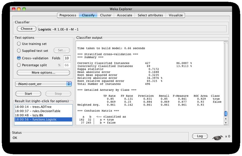
Figure 3.1: Weka Explorer
accessible through its built in graphical user interface shown in figure 3.1 or di-
rectly from any java program that includes its library. Therefore it is perfectly
well suited even for more sophisticated tasks in real world problems.
Being open source the actual versions of the source code as well as the compiled
versions of it for the most common platforms, including Windows, Mac OS X and
Linux2 , can be downloaded from its web page[25].
The rich set of functionality provided by the WEKA system includes [35]:
• Data preprocessing and visualization
• Attribute selection
• Classification algorithms (OneR, Decision trees, Covering rules)
• Prediction algorithms (Naı̈ve Bayes, Nearest neighbor, Linear models)
• Clustering (K-means, EM, Cobweb)
• Association rules
• Evaluation techniques
Despite that it offers so many different possibilities, the most important points
of the above list for this project are the attribute selection and various classifica-
tion and prediction algorithms. The later are used to analyze and classify/predict
2
The version used within this project is weka-3-6-2 for Mac OS XChapter 3. Background 10
on the input data, while the selection algorithms show which of the numerous fea-
tures contained in the input vector are involved in the decision making process
and which not.
Even though these points are the most important for the operational part of
the work, there is a need of the preprocessing step to prepare the data for the
classifiers as well as some evaluation techniques which allows to draw conclusions
on the quality of the result. These two functionalities are not directly related
to the machine learner itself, but they are needed for this work to justify the
obtained results.
One of the most important advantage of WEKA over most of the other tools
available is that the whole functionality of the system is available either over an
intuitive graphical user interface or via an API which allows to be called by a
normal (java)program. A second very important advantage that is used within
this project is the input data format used by WEKA which is ARFF. Having one
standardized file format for all the machine learning algorithms and all the other
tasks that can be performed with WEKA it is possible to have one single input
data set to try out all the possibilities offered. In this way it is possible within this
project to figure out the best suited machine learner for the underlying problem
of static source code analysis.
3.3.1 Machine Learning Algorithms
The WEKA framework categorizes its machine learning algorithms into 7 different
categories, which are “Bayes”, “Trees”, “Rules”, “Functions”, “Lazy”, “Misc”
and “Meta”. This section will not explain each algorithm present in the various
categories, but it gives an overview based on these groups and mentions their most
important algorithms. Detailed information on the algorithms can be obtained
from the book [35].
Bayes
This category contains mainly the bayesian network and various types of naı̈ve
bayes networks. Basically a bayesian network is a directed acyclic graph whose
nodes are variables, or in this case attributes, and the edges represent the condi-
tional probability associated with them. The naı̈ve versions of them are similar,
but based on a strong independence assumption. This means that they assume
that each feature in the set is independent from any other feature.
Trees
The most important trees implemented in WEKA are the “ADTree”, “Decision-
Stump”, “LMT”, “RandomForest” and “J48”. The latter is the java implemen-
tation of the “C4.5” which is well known in literature [27]. Logistic model treesChapter 3. Background 11 (LMT) are trees that apply logistic regression on their leave level, whereas a decision stump is a tree with just one level. Finally the ADTrees are alternat- ing decision trees, which alternate between decision levels (known values) and prediction levels (probabilities). Rules The algorithms present in this category include the “Decision Table”, which bases its decision on simple rule tables and “JRib” which implements the RIPPER [8] algorithm in Java. Furthermore it contains “NNge” which is a rule based implementation of the nearest neighbor algorithm. Functions This category contains mainly various algorithms based on a regression function like the linear or the logistic (These are called “Logistic”, “LinearRegression”). Both functions exist as “simple” versions (“SimpleLogistic” and “SimpleLinear- Regression”). Beside these group of learners it contains also the neural network “MultiLayerPerceptron” which is based on back propagation. Lazy In WEKA “lazy” is basically another word for nearest neighbor. Therefore this category contains the nearest neighbor algorithms “KStar”, “Ib1” and “Ibk” where the latter two differ only in the number of neighbors taken into consid- eration, while the former is based on a generalized distance function. Misc This category contains only two classifiers which are “Hyperpipes” and “VFI”(Voting Feature Intervals). These methods try to group the attributes of the training in- stances into intervals or ranges. These groups are then used in a nearest neighbour like fashion to determine the results. Meta The classifiers present in this category are not completely new but they use one (or more) of the classifiers present in the categories above and try to enhance its performance by using techniques like bagging, boosting or simply by combining classifiers. The most important ones in here are “Bagging” and “AdaBoostM1”. The latter is a boosting algorithm, that can dramatically increase the performance of a classifier, but may lead to overfitting [28].
Chapter 3. Background                                                                                                                12

3.3.2              Attribute Relation File Format (ARFF)
The attribute relation file format is a standardized format to represent data to-
gether with its name and type. As this format is used to feed every learner present
in the WEKA system it decouples data from the learner and creates in that way
the possibility of testing multiple learners as well as selection algorithms on a
single data file to determine the best suited method for the actual problem.
    Each ARFF file contains two distinct sections, that are called header and
data. The former contains the name of the relation and a list of attributes with
their associated types, whereas the latter consists of the real data vectors stated
in a CSV(Comma Separated Values) style. A short sample of such a file structure
taken from the book[35] is shown in listing 3.5
@RELATION i r i s

@ATTRIBUTE           sepallength              NUMERIC
@ATTRIBUTE           sepalwidth               NUMERIC
@ATTRIBUTE           petallength              NUMERIC
@ATTRIBUTE           petalwidth               NUMERIC
@ATTRIBUTE           class                    { I r i s −s e t o s a , I r i s −v e r s i c o l o r , I r i s −v i r g i n i c a }

@DATA
5 . 1 , 3 . 5 , 1 . 4 , 0 . 2 , I r i s −s e t o s a
4 . 9 , 3 . 0 , 1 . 4 , 0 . 2 , I r i s −s e t o s a
4 . 7 , 3 . 2 , 1 . 3 , 0 . 2 , I r i s −s e t o s a
...

                                                       Listing 3.5: ARFF Sample

    The header file in this case defines that the first four attributes are of type
“NUMERIC” meaning that the values in the data-part of the file can only consist
of numbers (or “?”, which in any case signals an unknown value) either floating
points or integers. The last attribute is of type “nominal”, which means that its
values can only consist of one of these stated in the attribute set.
    There exist some other possible types such as “STRING” for example where
every possible string can be its value. The selection of the types of the attributes
determines the set of possible machine learners that can work with it. The type
“STRING” for example is not possible for most of the learners simply because
they cannot handle it. Other learners instead can not deal with missing values
or have problems when they have to deal with “nominal” ones that either have
too few or too much different possible values.
Chapter 4
Problem Description
The topics of the above sections are mainly the different types of faults, a machine
learning framework (WEKA) and the analysis of static source code. Having this
knowledge in mind it is time to define what the real problem, focused within this
work, is.
Despite that, from the basic theory of computing we know that it is not possi-
ble to find and remove all bugs present in a reasonably large piece of software[15],
each developer tries to reduce their presence to an acceptable minimum. The
problem to face when searching for faults in source code is how this can be per-
formed in the most efficient way.
Static source code analysis is one possible solution to this problem with all its
pros and cons stated above. The most important advantage of this technique and
therefore probably the reason why it has been chosen so often in literature and
for this work too, is that it can be applied very early in the development process,
namely as soon as there is some code accepted by the corresponding programming
language compiler.
Even though it seems to be the best solution to reduce the number of bugs
in source code, it is a very annoying and time consuming activity when it has to
be performed manually. However when it can be done with the support of a well
suited tool it can be done in a more efficient way and so contribute to the overall
quality of the resulting software.
Nowadays the most widely used tools on the market are based on pattern
matching, which means that they are scanning the source code trying to iden-
tify faulty patterns by comparing them to the ones present in their database.
The problem with this approach is its inability to learn and adapt its behaviour
whenever a classification fails. This behaviour can lead to high number of false
positives which can highly devalue the usefulness of the tool (The impact of a
relatively high false positive rate has been investigated by Baca in [3]).
That is actually one of the points for having support of a machine learning
framework, which should be able to learn from previous classifications and there-
fore reduce the number of false positives while obtaining a high rate of true posi-
tives. The literature has shown in some papers that machine learning algorithms
can contribute to the quality of the results of static source code analysis tools.
13Chapter 4. Problem Description 14
The systematic literature review [33] performed prior to this work has shown that
most of the work performed so far deals with the prediction of faults in source
code using some kind of metrics (described in more detail in chapter 2 “related
works”), while there exist just a few papers about fault detection. The latter is
the area where this work is placed and the gap it tries to fill up is the absence of
a well suited method or approach to integrate a machine learning classifier into
the static analysis of source code.
The outcome of this work should be one possible solution of transforming a
standard C-language source code file into a format usable within the machine
learning framework. As stated already above this work will make use of the
WEKA framework, so the output of this step will be in form of an ARFF-file.
Having this conversion from source code to ARFF it should be possible to define
what kind of attributes or features are needed to identify the target faults within
the source and what kind of machine learning algorithms are really suitable for
this kind of operation.
These two questions are really crucial for the present work, being the main
drivers for the underlying investigation. In order to find the minimal or at least
one minimal set of features needed to identify faults in source code the experi-
ment has to be executed more than once. Starting with a large feature vector
extracted from the source code. Using the outputs provided by WEKA it should
be possible to understand which are the features that either are not used at all
by the classifiers or the ones that are used but could lead to misclassification.
Both of them will be removed in the subsequent iterations, which will hopefully
increase the precision of the suitable learners.
To answer to the second question it is needed to evaluate the possibility of
achieving a high fault detection rate with a small number of errors. This means
that the evaluation has to take care of the precision and the false positive/negative
rate of the resulting classifier to define its quality.Chapter 5
Proposed Solution
As seen in the chapter above the problem to face is to propose a solution for
feeding a machine learner with the data obtained by static source code to create
an intelligent fault detection method. This problem can be split into three sub
problems which are:
1. How to transform source code into a suitable format for the machine learning
classifier?
2. How to train that classifier? Which data has to be used to train it?
3. What are the features needed by the machine learner and which learner fits
best to the problem?
These are the main problems faced during this work and the solutions found
will be described in detail within this chapter. First it will present the prototypes
developed for the final solution then the method in which they are utilized to
produce the expected results.
Before coming to these sections there is one decision that had to be taken and
needs to be justified before starting to talk about the real solution itself. The
choice of the machine learning framework decides already about the file format of
its input files and needs to be defined therefore in advance. As already expectable
from the background chapter 3.3 the favorite choice was the WEKA data mining
framework. The main reason why it has been chosen beside its great popularity
in recent papers and its open source license was that it offers a wide variety of
different learners. Furthermore all the learners can be used with the same kind of
input file and using the same GUI which is already provided with the download
of the framework.
5.1 CMore
The first and probably the most complex prototype developed for this solution
is “CMore”. This program is able to decompose a program written in C into a
set of basic functions and procedures. The basic idea behind its functionality is
15Chapter 5. Proposed Solution 16
Figure 5.1: CMore: Abstract Execution Flow
that it should be able to follow the execution flow of a program and capture the
state of all the variables involved. Having all the states it is possible to detect
several kind of possible memory access faults which are null-pointer-references
and misuse of memory (see 3.2 for details)
The state diagram shown in figure 5.1 sketches the basic steps performed by
“CMore” to achieve this behaviour.
It mainly works in two steps, starting with a clean and divide preprocessing
step followed by the real state tracking step. The former activity is performed by
a set of classes of which the main one is called “FileWalker”. This class reads a
whole file as a string of bytes into its memory, which is needed to remove every
unused stuff from the file such as comments and macros1 . Afterwards the input
is subdivided into the various functions and procedures and stored into a central
depository (called “Brain”) for further use in the next steps.
Despite that its main functionality is to keep track of all the possible functions
and procedures, the repository contains a list of all known types, structures, con-
stants and global variables within the analyzed file. Furthermore there exists the
possibility of including other files into the execution flow, which in C is done like
this: #include "something.h". Whenever the “FileWalker” encounters such a
statement it launches a new instance of itself which is then responsible to decom-
pose the included file.
At the end of this step the central repository is aware of all the possible
function names together with their parameter list and all the possible types,
constants and globals.
Immediately after the preprocessing step the flow following step starts. In the
context of “CMore” the main classes involved are the “FormalExecuter” and the
1
As this is still a prototype the expansion and analysis of macros was left over as a future
workChapter 5. Proposed Solution 17
“ExpressionMelter”. The latter is responsible to evaluate possible mathemati-
cal expressions and replace variable names with their according values whenever
possible. The former class follows the execution flow and determines the nature
of each statement, which could be in this case an assignment, a declaration, a
function call or something else. This class has to be aware of the information
gained and invoke the protocolling of the state of the line when needed.
Protocolling in this context means to invoke the writing to a file in the format
the machine learning framework expects it. As seen in the background section 3.3
and shortly justified above the framework is WEKA and therefore the file format
has to be an ARFF-file.
@RELATION cmore
@ATTRIBUTE o p e r a t i o n { F u n c t i o n c a l l , Assignment , Usage}
@ATTRIBUTE l e f t t y p e {FILE , Function , header , char , i n t , Reference , Simple , void , . . . }
@ATTRIBUTE l e f t name {open , a l l o c , c l o s e , f r e e , gets , p r i n t f , seek , strdup , strcpy , strncpy ,
strcat}
@ATTRIBUTE l e f t i s R e f {true , false}
@ATTRIBUTE l e f t i s N u l l {true , false}
@ATTRIBUTE l e f t i s A s s {true , false}
@ATTRIBUTE l e f t i s U s e {true , false}
@ATTRIBUTE l e f t i s C h k {true , false}
@ATTRIBUTE r i g h t t y p e {FILE , Function , header , char , i n t , Reference , Simple , void , . . }
@ATTRIBUTE r i g h t name {open , a l l o c , c l o s e , f r e e , gets , p r i n t f , seek , strdup , strcpy , strncpy ,
strcat}
@ATTRIBUTE r i g h t i s R e f {true , false}
@ATTRIBUTE r i g h t i s N u l l { t r u e , false}
@ATTRIBUTE r i g h t i s A s s {true , false}
@ATTRIBUTE r i g h t i s U s e {true , false}
@ATTRIBUTE r i g h t i s C h k {true , false}
@ATTRIBUTE p a r 1 type {FILE , Function , header , char , i n t , Reference , Simple , void , . . . }
@ATTRIBUTE p a r 1 name {open , a l l o c , c l o s e , f r e e , gets , p r i n t f , seek , strdup , strcpy , strncpy ,
strcat}
@ATTRIBUTE p a r 1 isRef {true , false}
@ATTRIBUTE p a r 1 isNull {true , false}
@ATTRIBUTE p a r 1 isAss {true , false}
@ATTRIBUTE p a r 1 isUse {true , false}
@ATTRIBUTE p a r 1 isChk {true , false}
[..]
@ATTRIBUTE o r i g stmt STRING
@ATTRIBUTE e r r f r e e {true , f a l s e }
@DATA
Assignment , i n t , ? , t r u e , t r u e , f a l s e , f a l s e , f a l s e , R e f e r e n c e , ? , t r u e , f a l s e , f a l s e , t r u e , f a l s e
, ? , ? , ? , ? , ? , ? , ? , ? , ? , ? , ? , ? , ? , ? , ? , ? , ? , ? , ? , ? , ? , ? , ? , ? , ? , ? , ? , ? , ” c o = &cp ” , f a l s e
Assignment , i n t , ? , t r u e , t r u e , f a l s e , f a l s e , f a l s e , R e f e r e n c e , ? , t r u e , f a l s e , f a l s e , t r u e , f a l s e
, ? , ? , ? , ? , ? , ? , ? , ? , ? , ? , ? , ? , ? , ? , ? , ? , ? , ? , ? , ? , ? , ? , ? , ? , ? , ? , ? , ? , ”com = &p t r 1 ” , f a l s e
...
Listing 5.1: Snapshot of the final ARFF
Listing 5.1 shows a snapshot of the final ARFF file used to get the results for
the experiment described below. Its structure is quite simple and simulates the
typical structure of a possible statement. The first attribute states the kind of
operation the statement under investigation adheres to, which could be either an
“Assignment” a “Usage” or a “FunctionCall”. Depending on this attribute and
the real statement, one or more of the groups stated below it (“left”, “right”,
“par1”-“parX”) are filled. A group in such an ARFF file contains 7 attributes
and is separated by a blank line in listing 5.1 to make them identifiable more
easily. The last two attributes contain the real statement needed to identify the
faulty line in the code and the “error-free” flag.Chapter 5. Proposed Solution 18
The following examples should clarify the behaviour of the single groups and
why they are filled according to the statement:
a = b; −− > In this case “a” is used to fill the “left” and “b” to fill the “right”
group
aProcedure(a); −− > In this case “aProcedure” is the “right” and “a” is used
to fill “par1”
a = aFunction(b,c); −− > In this case “a” is “left”; “aFunction” is “right”
and “b”, “c” are the two parameters
The standardized structure of the ARFF file makes it easy later on to recon-
struct a statement using the instances present in the file. However one statement
can produce multiple instances in the result. The first case stated above would for
example produce one “Usage” instance for variable “b” and then an “Assignment”
instance for the assignment containing variables “a” and “b”.
One group of attributes in this file contains the following properties:
Type it contains the real type of a variable, if that type is known.
Name it is used to hold the name of the function in the case of a function call,
or in some cases the name of the actual variable
isRef Flag that tells if the variable is a pointer or a simple type
isNull If the variable is a reference it tells if it points to NULL
isAss Tells if the variable has been assigned to some value or address
isUse Tells if the variable has been used in any statement before
isChk Tells if the variables value has been checked before
5.2 Holmes
This program is not so complex and also not so important for the method itself,
but it gains some importance when it comes to the task of training the classifier.
“CMore”, the program described above, is not able to understand what an error
is, but it is able to keep track of the execution flow and provides later steps with
data. These steps now get only a list of instances and do not see the real source
code anymore, but they have to identify some instances as faulty whereas others
as fault-free. As the result of a conversion of a piece of source code into ARFF
can easily lead to several thousands of instances this could be a very annoying
process.Chapter 5. Proposed Solution 19
Figure 5.2: Holmes: Abstract Execution Flow
“Holmes” has been developed to simplify this process. It is able to perform
a line wise comparison of two ARFF files and separate matching lines from the
rest for any two ARFF files coming from “CMore”. The real purpose of having
a program performing this task will be explained later in this chapter when the
methodology is explained (see 5.3).
The basic execution steps of “Holmes” are shown in figure 5.2. At the be-
ginning it reads two versions of an ARFF file into its memory and sorts them
separately according to a predefined attribute consisting of the filename and the
statement which lead to the creation of the line.
Having these two files arranged in that way it is possible for “Holmes” to
determine if an instance (a line in the file) is present in either one of the two files
or in both. The latter case then needs to be analyzed further to determine if they
differ in some attributes or if the content of the line is exactly the same. The
latter is actually the only case in which the instances can be considered to be
the same, therefore “Holmes” will output them into a separate file. All the real
differences get an attribute appended which determines their origin (the input
file they are coming from).
As already mentioned above, the real purpose will be clearer after section 5.3,
however the idea behind is to create the needed instances to train a machine
learning classifier. Whenever this learning task should be performed there is a
need of having faulty instances together with its corrected versions, which can
be obtained from “CMore” described above in section 5.1. Despite that this
seems to be enough at first sight, “CMore” is not searching for faults and will
therefore output all the data it is expected to output for both, the faulty and the
corrected version. These two output files will of course contain many duplicateChapter 5. Proposed Solution 20
Figure 5.3: Method
lines, as the correction of a fault does usually not cause the whole program to
change. “Holmes” in this scenario simplifies the detection of the instances that
are relevant for the training step.
5.3 Methodology
Now that the most important programs used during the work are introduced it
comes to the experiments where they are used in conjunction to gain the results.
The general structure of the process applied in order to get them is shown in
figure 5.3 and described more in detail below.
Starting from the basic idea of combining modern machine learning algorithms
with the field of static source code analysis the first step was to investigate what
has already been analyzed and published and where there could be a possible gap
to fill. In order to get this information a deep study of all the possible (and freely
available) papers published in this area has been performed and summarized in
a systematic literature review [33].
Despite that this review has been written prior to this thesis it can be seen
as the first step and the source of the gap that this work tries to fill (The most
important findings of the review have been stated in the related works chapter
2). From the results of this review the main objectives and its correlated research
questions have been drawn (These are stated in the introduction chapter 1 and
described more in detail in chapter 4 “problem description”).
At this point the problem has been clearly defined in terms of research ques-
tions and objectives and lacked of possible solutions. The proposed one in this
case was the development of a program that is able to keep track of the status
information of every variable in an execution flow. The prototype capable ofChapter 5. Proposed Solution 21
performing this task has been called “CMore” and is described in detail above.
The next step in this flow was to define a strategy to evaluate the possibilities
behind this solution and to find possible improvements. Therefore the idea was to
evaluate the suitability of the machine learning algorithms in this case by testing
them on real open source projects. In order to be suitable for the purpose of the
work the chosen projects needed to have some kind of bug-repository and their
source has to be accessible via some common version control system2 . Projects
that fulfill these requirements can be found either on Sourceforge[31] or on Google
Code[7].
Having these projects it was possible to create different “CMore” output files
for the different versions on the version control system in order to obtain source
containing a certain fault and code without the fault. Whenever it was not
possible to locate the fault in the source code, or the bug repository did not
provide enough information the solution was to inject a suitable fault directly in
the source code to come up with the two different versions. These two versions
were then used as inputs for “Holmes” to get the interesting instances out from
the two files produced by “CMore” that really identify the fault. These instances
have then been collected to obtain a huge file of instances needed in the next step
(A more detailed description of “CMore” and “Holmes” can be found above in
this chapter).
The result from the previous step was a huge file of instances that has then
been used to train the machine learner. In the case of WEKA it was now possible
to train many different learning algorithms with this file, and that is one of its
advantages that made it suitable for this work. The WEKA output of the various
learners has then been collected and analyzed more in detail. The results of this
analysis will be shown in the results chapter 6.
To test if all the features in the set used for the analysis are needed it has
been reduced by some hopefully unnecessary attributes and then re-evaluated
using the WEKA framework. The results of this part of the experiment will be
shown as well in the results chapter 6.
As a last step the best machine learners have been tested on the complete out-
put of one of the open source projects previously used to generate the training set
for the learners, to evaluate its performance on a real data set. This experiment
should show that the classifiers trained are not working only in the suitability
environment but also in a real world scenario.
5.3.1 Experimental Design
The main idea behind this study is to show that the presented approach works for
the field of fault detection. In order to show this a test scenario will be created
and subsequently analyzed and evaluated.
2
SVN[32], CVS[9] or GIT[13]Chapter 5. Proposed Solution 22
X O
X = Treatment −> fault detection
O = Observation −> Accuracy, FP, FN
Subjects −> Operations (Faulty/Correct Instances)
The best suited experimental design for this kind of evaluation is the “One
Shot Case Study” whose structure is sketched above. This design starts directly
with the treatment omitting the pre-observation/testing and postpones the test-
ing to the end of the study.
In this case the treatment is the whole training procedure of the machine
learners which includes the creation and manual classification of the instances
used for training. As soon as the training is completed the suitability analysis is
performed which returns the list of suitable learners by analyzing their accuracy,
false positive rate and false negative rate. The project evaluation study follows
the same procedure, however in this case it can be seen as a further testing or
observation.Chapter 6
Results and Analysis
In this chapter the most important results are shown in terms of tables and graphs.
Due to space constraints, some of them are truncated to focus on the interesting
parts for the conclusions drawn, but in any case a complete reference of the data
obtained by the different experiments can be found in the appendix A. Wherever
a truncation has been applied there will be a reference to the corresponding data
set in the appendix.
From the methodology it is possible to see that two different experiments have
been performed whose results will be explained in two different sections within
this chapter. However before coming to the real results there will be a short
introduction of the projects used to come to the results.
6.1 Open Source Projects
As already stated shortly in the methodology the best sources for projects fulfilling
the requirements to be considered can be found either on Sourceforge[31] or on
Google Code[7].
The requirements for the projects are the following:
Language The programs should be written entirely or at least mostly in C pro-
gramming language
Availability The prototypes need real source code, so it should provide access
to that using one of the following common version control systems SVN[32],
CVS[9] or GIT[13]
Bug Repository The programs should provide access to a bug database if pos-
sible
Project Size As the programs used to extract the data are only prototypes the
programs under investigation should be of small or medium size
During the search it was possible to come up with 6 candidates for the deeper
investigation, which are:
23Chapter 6. Results and Analysis 24
Algoview a small program that is able to visualize a program as a graph (Source-
forge)
Boxc is a vector graphics language to simplify their creation (Sourceforge)
ClamAV is an anti-virus program developed for the Linux environment (Source-
forge)
PocketBook is an open source firmware for e-book readers (Sourceforge)
FalconHTTP is a HTTP server offering several parallelism technologies (Google
Code)
Siemens Programs is a collection of programs with several versions where for
educational purposes some faults have been introduced (Other [26] )
6.2 Suitability Analysis Results
From the programs stated above it has been possible to extract correct and faulty
instances using the two programs “CMore” and “Holmes” as described in the
methodology section (see 5.3).
In total it was possible to get 496 instances containing faulty and correct
versions of instances and some correct instances reflecting the most important
standard situations. The latter have been added in order to reduce the false
alarms on correct standard situations in source code (important for the second
experiment). The results of the various WEKA machine learning algorithms when
trained with these instances are stated below.
According to the literature review performed beforehand the crucial values to
measure the performance of a static analysis method are:
Accuracy which is the percentage of correctly classified instances
False Positive rate is the percentage of instances the method signals as faulty
among the correct ones
False Negative rate is the percentage of instances signaled as fault free among
the faulty ones
In order to obtain these measures the instances are loaded into WEKA using
the WEKA explorer and evaluated against the possible machine learning algo-
rithms. In order to get a representative evaluation a cross-validation with 10 folds
has been chosen. This means that the whole data set is randomly divided into 10
different sets of which 9 are used to train and the remaining to test the classifier.
This procedure is then repeated 10 times, so each set will be once the test set.Chapter 6. Results and Analysis 25
The whole procedure has been performed twice to reduce the set of features
involved in the process. The purpose of this should be to understand which
features are really needed to identify the faults in the source. After the first run
the log-data of the classifiers has been analyzed to understand which features are
not used at all or which of them could probably lead to incorrect classifications
when used in the decision process of the learners. Those features have been
reduced in the second run, trying to improve the learners performance.
This experiment is intended to proof the suitability of certain machine learning
algorithms to the underlying data set.
6.2.1 Accuracy
Despite that it took some time, WEKA made it quite easy to test and compare
about 71 classifiers, which means all the classifiers that are applicable with the
kind of data produced by “CMore”. The resulting ranking in terms of accuracy
is shown in figure 6.1.
Figure 6.1: Accuracy (Full) Figure 6.2: Accuracy (Reduced)
It is truncated to show only the ones that performed better than 90%, however
the complete data set is listed in the appendix A, table A.1. In this graph among
the 7 classifiers performing better than 95%, three are based on nearest neighbor
algorithms (“Ib1”, “Ibk”, “NNge”), three are tree based (“LMT”, “RotationFor-
est” and “ADABoost” performed on a “BFTree”) and the function based neural
network “MultiLayerPerceptron”.
Despite that trees perform quite well on the given data set the output of
the attributes they used showed most of the times that they tried to base their
reasoning on the real data type of the involved variables. To test their reactionChapter 6. Results and Analysis 26
Figure 6.3: Average Accuracy per Category
and the one of the other learners in the second step of this experiment these
features have been removed. The output in terms of accuracy of this experiment
is shown in figure 6.2 (complete data set is listed in the appendix A, table A.1).
As expected the performance of the trees has been reduced and also the pre-
viously well performing “ADABoost” was not able to push it back to the top.
However it was possible to increase the performance of the “MultiLayerPercep-
tron” to be the overall highest in the experiment together with the “NNge” nearest
neighbor learner.
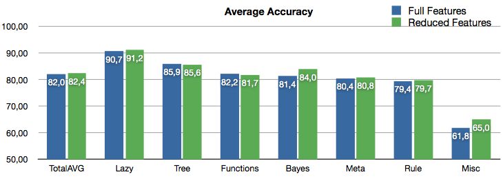
This impression is acknowledged by figure 6.3 which shows the average accu-
racy per category (These categories are taken from the categories used in WEKA
to separate the various classifiers). It shows that almost all categories could
improve by not taking in consideration the real name of the involved types, ex-
cept the trees. The graph shows also that functions could not improve, but this
is manly due to a high loss in accuracy of one learner in this category called
“SMO(Puk)1 ” which decreased from almost 95% down to 66%. On the other
hand one of the new best performing learners descends from this category too.
6.2.2 False Positive Rate
A similar impression can be gained from the false positive analysis results shown
in figure 6.4 for the full feature set and figure 6.5 for the reduced one. Among
the bests for the full data set there is still the nearest neighbor algorithm and
the “MultiLayerPerceptron” together with the ADAboosted “BFTree” and some
other trees like the “LMT” and a version of the “J48”. As before when using
the reduced feature set the trees will become worse, but the nearest neighbor
algorithms and the “MultiLayerPerceptron” gain.
This impression is again acknowledged by the averages per category which
show that all except the trees could gain from the reduced feature set (see figure
6.6).
Interesting in this case is that the “NNge” nearest neighbor algorithm despite
1
Sequential minimal optimisation using the “Puk” kernel (Support Vector Machine)You can also read