Phylogeography of the iconic Australian pink cockatoo, Lophochroa leadbeateri
←
→
Page content transcription
If your browser does not render page correctly, please read the page content below
Biological Journal of the Linnean Society, 2021, 132, 704–723. With 4 figures.

Phylogeography of the iconic Australian pink cockatoo,
Lophochroa leadbeateri
KYLE M. EWART1,2,*, , REBECCA N. JOHNSON1,2, LEO JOSEPH3, , ROB OGDEN4,
GRETA J. FRANKHAM2,5 and NATHAN LO1

                                                                                                                             Downloaded from https://academic.oup.com/biolinnean/article/132/3/704/6121450 by guest on 25 March 2021
1
  School of Life and Environmental Sciences, The University of Sydney, Sydney, NSW 2006, Australia
2
  Australian Centre for Wildlife Genomics, Australian Museum Research Institute, Sydney, NSW 2010,
Australia
3
  Australian National Wildlife Collection, National Research Collections Australia, CSIRO, Canberra,
ACT 2601, Australia
4
  Royal (Dick) School of Veterinary Studies and the Roslin Institute, University of Edinburgh, Edinburgh
EH25 9RG, UK
5
  Centre for Forensic Science, University of Technology Sydney, PO Box 123, Broadway, NSW 2007,
Australia

Received 7 September 2020; revised 9 December 2020; accepted for publication 11 December 2020

The pink cockatoo (Lophochroa leadbeateri; or Major Mitchell’s cockatoo) is one of Australia’s most iconic bird
species. Two subspecies based on morphology are separated by a biogeographical divide, the Eyrean Barrier.
Testing the genetic basis for this subspecies delineation, clarifying barriers to gene flow and identifying any
cryptic genetic diversity will likely have important implications for conservation and management. Here, we
used genome-wide single nucleotide polymorphisms (SNPs) and mitochondrial DNA data to conduct the first
range-wide genetic assessment of the species. The aims were to investigate the phylogeography of the pink
cockatoo, to characterize conservation units and to reassess subspecies boundaries. We found consistent but
weak genetic structure between the two subspecies based on nuclear SNPs. However, phylogenetic analysis
of nuclear SNPs and mitochondrial DNA sequence data did not recover reciprocally monophyletic groups,
indicating incomplete evolutionary separation between the subspecies. Consequently, we have proposed that
the two currently recognized subspecies be treated as separate management units rather than evolutionarily
significant units. Given that poaching is suspected to be a threat to this species, we assessed the utility of our
data for wildlife forensic applications. We demonstrated that a subspecies identification test could be designed
using as few as 20 SNPs.

ADDITIONAL KEYWORDS: conservation genetics – Lophochroa leadbeateri – phylogeography – population
genomics – wildlife forensics – wildlife trade.

                    INTRODUCTION                                    occurs in low densities throughout Australia’s harsh
                                                                    arid and semi-arid regions.
The pink cockatoo (also known as Major Mitchell’s
                                                                      Within the wide yet patchy distribution of the pink
cockatoo), Lophochroa leadbeateri (Vigors, 1831),
                                                                    cockatoo, four core breeding regions are apparent
is an iconic bird species endemic to Australia. It
                                                                    (Blakers et al., 1984; Fig. 1A). Although previous
is considered by many to be the most beautiful and
                                                                    authors have recognized a variable number (zero to
spectacular of the cockatoos (Cacatuidae; Rowley &
                                                                    four) of subspecies (e.g. three subspecies, Mathews,
Chapman, 1991; Schodde, 1994), having pink-white
plumage and an impressive bright red, yellow and                    1912; four subspecies, Peters, 1937; no subspecies,
white crest. The pink cockatoo is a hardy species that              Condon, 1975; three subspecies, Hall, 1974; two
                                                                    subspecies, Schodde, 1997), two subspecies, Lophochroa
                                                                    leadbeateri leadbeateri and Lophochroa leadbeateri
*Corresponding author. E-mail: kyle.ewart@austmus.gov.au            mollis (cf. Forshaw & Cooper, 1981) have generally

© 2021 The Linnean Society of London, Biological Journal of the Linnean Society, 2021, 132, 704–723                  704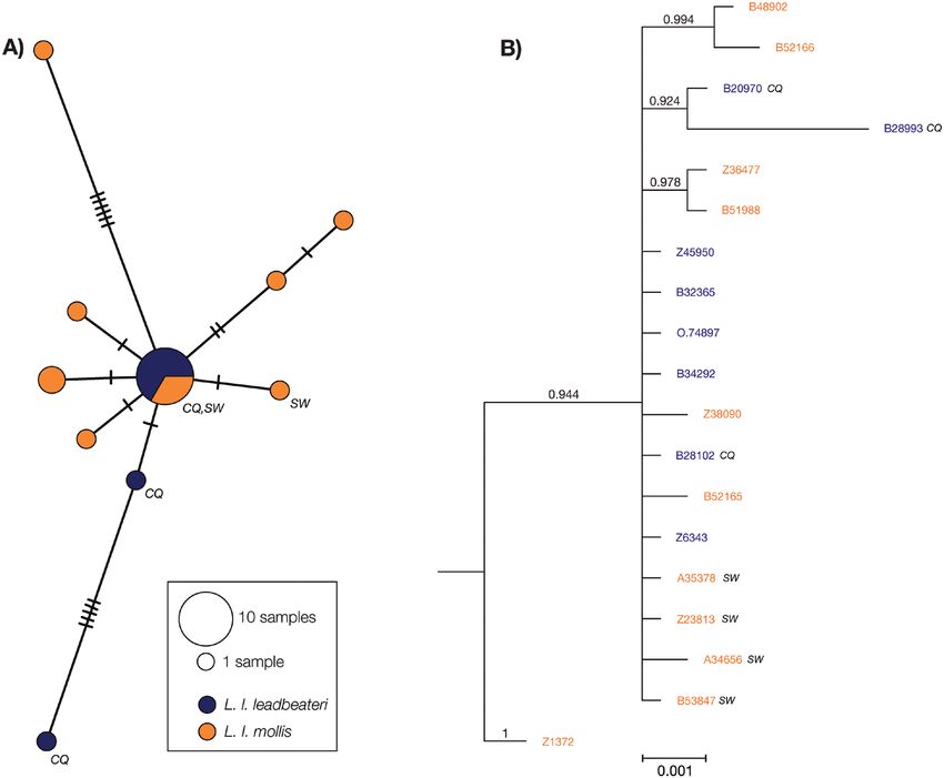
PHYLOGEOGRAPHY OF THE PINK COCKATOO 705
Downloaded from https://academic.oup.com/biolinnean/article/132/3/704/6121450 by guest on 25 March 2021
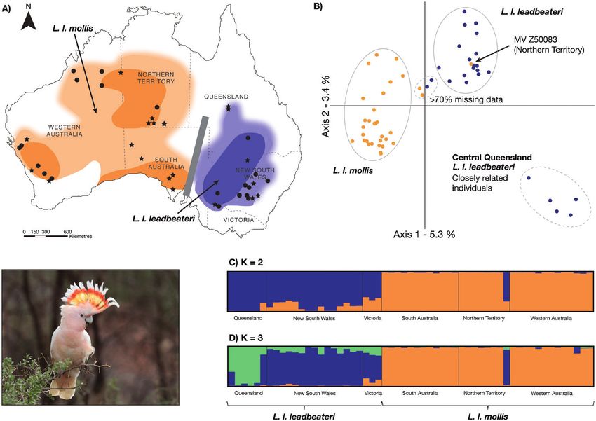
Figure 1. A, the distribution of Lophochroa leabeateri leadbeateri (blue) and Lophochroa leabeateri mollis (orange) in
Australia, adapted from Schodde (1994) and Menkhorst et al. (2017), and localities of the frozen tissue samples (stars)
and toe pad samples (circles) genotyped in this study. The thick grey line represents the Eyrean Barrier, the darker
shading represents core breeding zones, and the lighter shading and blurred fringes represent areas of potentially sparser
distribution and/or non-breeding, based on records from the Atlas of Living Australia database (https://www.ala.org.au;
accessed 4 November 2020). B, a principal coordinates analysis plot for 57 pink cockatoo individuals using 4135 single
nucleotide polymorphisms (SNPs). C, D, STRUCTURE plots for 57 pink cockatoo individuals based on 2131 SNPs when
K = 2 and K = 3, respectively. The bottom left photograph is of Lophochroa leabeateri leadbeateri, Mt. Hope, NSW, Australia.
Photograph by Corey Callaghan.
been accepted since the publication of the study by distribution, it is listed as Vulnerable (New South
Schodde (1994) (Fig. 1A) on the basis of body size and Wales and Queensland: NSW State Government, 2016;
colour and the pattern of the crest. These subspecies Queensland State Government, 2006) or Threatened
are separated by the Eyrean Barrier (Fig. 1A), which (Victoria; Victorian State Government, 1988; Walker
is a well-documented biogeographical barrier in et al., 1999) (for state localities, see Fig. 1A). The species
southern Australia for a range of bird species (Ford, abundance and range in north-western Victoria and
1974; Schodde, 1982; Kearns et al., 2009; Dolman & western New South Wales have been greatly reduced
Joseph, 2012). Lophochroa leadbeateri leadbeateri through the removal of habitat; in particular, the loss
is found east of the Eyrean Barrier and has a more of hollow-bearing trees (Garnett et al., 2011). Like other
prominent yellow band in its crest and is larger in cockatoo species, the pink cockatoo is unable to excavate
body size, whereas L. l. mollis is west and north of its own hollows for nesting and therefore requires
the Eyrean Barrier (Schodde, 1994, 1997; Forshaw & naturally occurring tree hollows (Mackowski, 1984;
Cooper, 2002). Cameron, 2007). Furthermore, increased agriculture and
Despite its wide distribution, the pink cockatoo clearing of feeding habitat have impacted the species,
is of conservation concern. In the eastern part of its particularly in the south-west of its range in the Western
© 2021 The Linnean Society of London, Biological Journal of the Linnean Society, 2021, 132, 704–723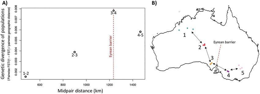
706    K. M. EWART ET AL.

Australian wheat-belt region (Rowley & Chapman, 1991).          2020). Furthermore, genetic data could facilitate
Another threat to this species is poaching (Forshaw &           the development of wildlife forensic tools, such as
Cooper, 1981; Higgins, 1999), which Rowley & Chapman            geographical provenance and progeny testing, to
(1991) found to impact the most critical stage of the           increase the capacity for detection and prosecution
life cycle, i.e. recruitment of young. Poaching is directly     of trafficking crimes involving this species (Walker
linked to demand for the species in the illegal pet trade.      et al., 1999; Huffman & Wallace, 2011). The pink
Together, these factors indicate a need for improved            cockatoo is listed under CITES Appendix II, and trade
understanding of phylogeographical patterns within the          in the species is strictly regulated under Australian
species to aid in the conservation management of the            legislation.
species.                                                           H e r e, w e p e r f o r m t h e f i r s t c o m p r e h e n s i v e
   Genomic tools allow researchers to investigate how           phylogeographical assessment of the pink cockatoo to

                                                                                                                                          Downloaded from https://academic.oup.com/biolinnean/article/132/3/704/6121450 by guest on 25 March 2021
genetic diversity is distributed among populations.             address the topics we have raised above. This builds on
They can help to identify and manage at-risk                    two earlier genetic studies involving this species based
populations. Characterization of discrete units of              on allozymes (Adams et al., 1984) and a multilocus
genetic variation, termed conservation units (Ryder,            nuclear and mitochondrial DNA (mtDNA) dataset
1986), and clarification of barriers to gene flow               (White et al., 2011); both used only a few individuals
within the pink cockatoo will facilitate conservation           to address the systematic position of the species with
strategies that maximize the evolutionary potential             respect to other cockatoos. Pink cockatoo specimens
of the species (Frankham et al., 2010). The putative            from across the species range have been collected over
subspecies barrier, the Eyrean Barrier, comprises               many decades and are stored in museums throughout
the Flinders Ranges and Lake Eyre Basin (Schodde,               Australia and elsewhere. Owing to developments
1982). It is thought to have limited dispersal during           in museum genomics, genome-wide data for use in
the Plio-Pleistocene owing to the presence of vast              population-level studies can be generated from old
lakes associated with the Lake Eyre Basin, and then             museum specimens (Rowe et al., 2011; Ewart et al.,
in the Pleistocene owing to extreme aridity (Ford &             2019). We generated thousands of genome-wide single
Parker, 1973; Ford, 1974; Schodde, 1982; Joseph et al.,         nucleotide polymorphism (SNP) markers and sequence
2006). However, the timing and strength with which              data at three mtDNA markers from pink cockatoo
the Eyrean Barrier has separated populations within             frozen tissue and toe pad samples across their entire
species is known to vary between avian taxa (Schodde,           distribution. We performed comprehensive population
1982; Dolman & Joseph, 2012; McElroy et al., 2018).             genomic analyses to investigate potential barriers
Whether the morphological differences between pink              to gene flow for the purposes of clarifying taxonomy
cockatoo subspecies at this barrier reflect underlying          and informing conservation management. These data
genetic divergence and potential conservation units             can be interpreted in light of the biogeography and
is unknown. Schodde (1994) suggested that there                 palaeoenvironmental history of the arid and semi-arid
is currently no dispersal between subspecies over               zones of Australia and compared with the steadily
this barrier, and that the two might even warrant               increasing body of phylogeographical analyses of
recognition at species rank. Furthermore, it is unknown         species having broadly similar distributions across
whether cryptic genetic structure exists across other           southern Australia (Neaves et al., 2009; Dolman &
well-characterized southern Australian arid zone                Joseph, 2012, 2015; Engelhard et al., 2015; Ansari
biogeographical barriers within the pink cockatoo               et al., 2019).
distribution, such as the Nullarbor and Murravian
Barriers (see Schodde & Mason, 1999). The impact
of these biogeographical barriers varies considerably
between species (Neaves et al., 2012).                                        MATERIAL AND METHODS
   Clarification of the evolutionary history of the
species and intraspecific taxonomy have been                         Sample acquisition and DNA extractions
problematic owing to a combination of poor sampling,            We acquired pink cockatoo frozen tissue (frozen
relatively weak morphological divergence across                 liver/muscle; N = 45) and toe pad (N = 51) samples
the species (e.g. see Forshaw, 2011) and the need to            from across their distribution (Fig. 1A; Supporting
disentangle patterns of geographical, sexual and age-           Information, Table S1). Samples were obtained from:
related variation. Genomic analyses have the potential          the Australian National Wildlife Collection, Canberra
to help to characterize conservation units, investigate         (ANWC); the Australian Museum, Sydney (AM);
connectivity among core breeding populations and                Museum Victoria, Melbourne (MV); and the Western
resolve lingering taxonomic uncertainties about                 Australian Museum, Perth (WAM). Collection dates for
subspecies boundaries (Baumsteiger et al., 2017;                these samples ranged from 1883 to 2011 (Supporting
Marie et al., 2019; Tonzo et al., 2019; Ewart et al.,           Information, Table S1).

                           © 2021 The Linnean Society of London, Biological Journal of the Linnean Society, 2021, 132, 704–723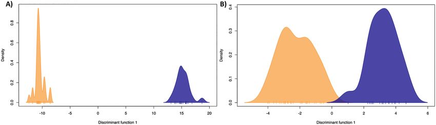
PHYLOGEOGRAPHY OF THE PINK COCKATOO                    707

   Thinly sliced toe pads (~2 mm thick) were sampled                 Single nucleotide polymorphism filtering
from traditional museum specimens, and DNA was                   We applied numerous SNP filtering criteria depending
extracted following the method described by Ewart                on the analysis (following Ewart et al., 2019). First,
et al. (2019). These DNA extractions were performed              we removed the duplicate/triplicate samples with the
in a clean room facility dedicated to historical                 highest amount of missing data. Second, we removed
museum samples likely to have degraded DNA.                      potentially erroneous SNPs and SNPs with a high level
Genomic DNA was extracted from frozen tissue                     of missing data, based on reproducibility (100%) and
samples following the manufacturer’s protocols for               call rate (> 80%), using the R package dartr v.1.0.5
the ‘Bioline Isolate II Genomic DNA kit’ Bioline                 (Gruber et al., 2018). Third, to meet the population
(Australia). The DNA concentration was measured                  genetic assumptions of some analyses, we removed
using a Qubit 2.0 Fluorometer (Thermo Fisher                     linked SNPs, outlier SNPs that potentially represented

                                                                                                                            Downloaded from https://academic.oup.com/biolinnean/article/132/3/704/6121450 by guest on 25 March 2021
Scientific).                                                     loci under selection and SNPs out of Hardy–Weinberg
                                                                 equilibrium (HWE). To remove linked SNPs to
                                                                 meet the assumption of linkage disequilibrium for
  Single nucleotide polymorphism genotyping                      some of the analyses, we retained only one SNP
Single nucleotide polymorphism data were generated               per DArTseq locus using the R package dartr . To
using DArTseq, a reduced representation sequencing               identify and remove outlier SNPs that are potentially
method (methods described by Kilian et al., 2012; Cruz           under directional or balancing selection to meet the
et al., 2013). This was performed by Diversity Arrays            assumption of neutrality for some analyses, we used
Technology (DArT) in Canberra, ACT, Australia.                   LOSITAN (Beaumont & Nichols, 1996; Antao et al.,
DArTseq has previously been used to generate SNP                 2008). For this analysis, samples were divided into
data for a range of phylogeographical, phylogenetic              subspecies; then we performed 100 000 simulations,
and population genetic studies on vertebrate species             applying the ‘infinite alleles’ mutation model, a 0.95
(Melville et al., 2017). Briefly, different combinations         confidence interval and a 0.1 false discovery rate. To
of restriction enzymes were tested, and the PstI-                identify departure from HWE, we used ARLEQUIN
SphI enzymes were selected for digestion of cockatoo             v.3.5 (Excoffier & Lischer, 2010), implementing
DNA. DNA was then processed according to the                     1 000 000 Markov chain steps and a burn-in of 100 000.
method of Kilian et al. (2012), using two different              We removed loci with a P-value < 0.01 that potentially
adaptors that correspond to the restriction site                 deviate from HWE. For this analysis, we considered
overhangs, both containing an Illumina flow cell                 all samples as one population, which is likely to be a
attachment sequence, and one (the PstI-compatible                conservative approach, because we would expect some
adapter) also containing a sequencing primer                     false positives owing to the Wahlund effect.
sequence and variable-length barcode region. The                    To investigate whether remnant poor-quality SNPs
library was subjected to polymerase chain reaction               were skewing results, additional filters were applied to
(PCR; using REDTaq DNA Polymerase; Sigma-                        represent a ‘stringently filtered’ dataset, and analyses
Aldrich) as follows: initial denaturation at 94 °C for           were repeated. Here, we filtered SNPs for average
1 min, followed by 30 cycles of 94 °C for 20 s, 58 °C            locus coverage (> 20) using the R package dartr ,
for 30 s and 72 °C for 45 s, with a final extension step         and minor allele frequency (MAF; > 0.05) using the R
at 72 °C for 7 min. The library was then normalized              package poppr v.2.6.1 (Kamvar et al., 2014, 2015).
and sequenced by first performing a c-Bot (Illumina)                Additionally, to ensure that the inclusion of toe pad
bridge PCR, followed by single end sequencing for 77             samples from old museum specimens did not skew
cycles on an Illumina Hiseq2500.                                 results, SNPs were re-called using only the more
   The resultant short-read sequences were processed             contemporary tissue samples (using the SNP calling
using the DArT analytical pipelines. First, poor-                methods outlined in the previous section). The SNPs
quality sequences were removed (using a Phred                    were subsequently refiltered. Additional details on
score ≥ 10), and sequences were demultiplexed (using             SNP filtering methods and variants are provided in
a barcode Phred score ≥ 30). Second, sequences were              the Supporting Information (Appendix S1).
trimmed to 69 bp and clustered with a Hamming
distance threshold of three. Low-quality regions from
singleton tags were corrected where possible. Third,                  Single nucleotide polymorphism quality
SNPs were called using the proprietary DArTsoft14                                          control
SNP calling pipeline. Real alleles were discriminated            To quantify genotyping error, we included 18 replicate
from paralogous sequences by assessing a range of                and four triplicate samples among the 96 pink
parameters, including sequence depth, allele count               cockatoo samples analysed (indicated in Supporting
and call rate.                                                   Information, Table S1). We used various replicate/

© 2021 The Linnean Society of London, Biological Journal of the Linnean Society, 2021, 132, 704–723
708 K. M. EWART ET AL.
triplicate types to investigate the factors that might First, genetic variation was summarized and
influence error, including: frozen tissue replicates visualized using a principal coordinates analysis
(from the same and different DArTseq plates), toe (PCoA). This was performed using the R packages
pad replicates (from the same and different DArTseq dartr and ade4 v.1.7 (Chessel et al., 2004).
plates), frozen tissue/toe pad replicates (a frozen Second, STRUCTURE v.2.3 (Pritchard et al.,
tissue and toe pad from the same individual) and 2000) was used to investigate genetic structure
tissue DNA replicates (from the same and different and admixture. For this analysis, we modelled up to
DArTseq plates). five ancestral populations (K = 1–5), implementing
We calculated SNP error rates (i.e. the number ten replicates for each K, assuming admixture and
of SNP mismatches between replicate pairs over correlated allele frequencies (Porras-Hurtado et al.,
the total number of SNPs that were not missing in 2013). We ran the analysis for 2 million iterations with
Downloaded from https://academic.oup.com/biolinnean/article/132/3/704/6121450 by guest on 25 March 2021
both replicates) using R functions from the study a burn-in of 1 million. This analysis was parallelized
by Mastretta‐Yanes et al. (2015). Error rates were and automated using S tr A uto v.1.0 (Chhatre &
calculated before and after SNP filtering. Emerson, 2017). We considered six different estimators
to determine the optimal value of K, generated using
S tructure S elector (Li & Liu, 2018). Replicate
Generation of mitochondrial DNA sequence runs were merged, and bar plots were generated
data using Clumpak (Kopelman et al., 2015), implemented
To generate mitochondrial reference genomes, we through StructureSelector. We took a hierarchical
performed low-coverage whole genomic sequencing for approach, whereby the population clusters identified
four pink cockatoo samples (indicated in Supporting using the full dataset were separated, refiltered, then
Information, Table S1), following the NEBNext DNA run independently.
library preparation protocol, with a pretreatment of Third, to investigate whether patterns of genetic
500 bp shearing using Covaris M220. The libraries differentiation were derived from continuous
were then sequenced on an Illumina MiSeq using (i.e. isolation by distance; IBD) or discrete (e.g.
paired-end 251 bp sequencing. Library preparation biogeographical barriers) phylogeographical
and sequencing were performed at the Monash processes, we performed a con S truct analysis
University Malaysia Genomics Facility (Selangor, (Bradburd et al., 2018), implementing the spatial
Malaysia). The resultant paired sequence reads were model. A con S truct (i.e. ‘continuous structure’)
trimmed using the BBDuk plugin in GENEIOUS analysis is similar to the STRUCTURE analysis, but
v.10.2.4 (Kearse et al., 2012), then assembled using controls for geographical distance between samples.
GENEIOUS and NOVOP lasty (Dierckxsens et al., Based on initial optimization, we ran two independent
2017). We then designed primers for the ND4 and conStruct analyses, with the ‘adapt delta’ parameter
ND5 genes and d-loop (for ND2, we used primers from (the target average proposal acceptance probability)
the study by Sorenson, 2003), and we amplified and set to 0.85, implementing two chains with 100 000
sequenced 15 samples from across the pink cockatoo Markov chain Monte Carlo (MCMC) iterations
range (indicated in Supporting Information, Table S1). for each run. We checked for consistency between
Thus, the mtDNA analyses were carried out using chains and independent runs, and checked visually
19 samples (four using low-coverage whole genomic for convergence using the trace plots generated by
sequencing and 15 using Sanger sequencing). The con S truct . To determine an appropriate level of
d-loop marker was subsequently excluded because parameterization, we ran five replicates of a cross-
it was not possible to sequence it reliably (possibly validation analysis comparing the spatial and non-
owing to the presence of control region duplications, spatial models for K = 1–5 for each replicate. We used
which are often found in parrot species; Schirtzinger a random 90% subsample as the training partition and
et al., 2012; Eberhard & Wright, 2016). Additional ran the analysis for 10 000 MCMC iterations.
details on mitochondrial genome assemblies, primers, Fourth, to measure genetic divergence between
PCR conditions and sequencing can be found in the subspecies, we calculated pairwise fixation index
Supporting Information (Appendix S2). (F ST) values (Weir & Cockerham, 1984) using the R
package hierfstat v.0.4.22 (Goudet & Jombart, 2015).
The F ST values were considered significant if their
Identification of population structure associated confidence intervals (based on 0.025 and
We used five methods to investigate the population 0.975 quantiles, implementing 1000 bootstraps) did
structure present in the SNP genotype data. Details not encompass zero.
of the different SNP filtering strategies and samples Fifth, to investigate differentiation within and
used in the different analyses are provided in the between subspecies, we performed an analyses of
Supporting Information (Appendix S1; Table S1). molecular variance (AMOVA) using the R package
© 2021 The Linnean Society of London, Biological Journal of the Linnean Society, 2021, 132, 704–723PHYLOGEOGRAPHY OF THE PINK COCKATOO 709
poppr and checked for significance using 10 000 Genetic diversity
permutations implemented in the R package ade4. To To measure the genetic diversity within each subspecies,
investigate whether any genetic structure patterns we calculated allelic richness, heterozygosity and
in the above analyses were driven by closely related private allele counts for each SNP marker. Allelic
individuals (e.g. cousins), we performed an inter- richness was calculated using the R package
individual kinship analysis using the R package PopGenReport v.3.0.4 (Adamack & Gruber, 2014),
SNPRelate v.1.14 (Zheng et al., 2012). implementing rarefaction to account for differences
We performed a haplotype network analysis to in sample size. Observed and expected heterozygosity
investigate population structure within the mtDNA w e r e c a l c u l a t e d u s i n g G e n A l E x ( Pe a k a l l &
sequence dataset. We performed this analysis using Smouse, 2006, 2012). A count of private alleles per
popart (Leigh & Bryant, 2015), based on concatenated population was calculated using the R package poppr.
Downloaded from https://academic.oup.com/biolinnean/article/132/3/704/6121450 by guest on 25 March 2021
ND2, ND4 and ND5 sequences (a total of 2037 bp) and Mitochondrial DNA diversity was measured in terms
19 samples, implementing the statistical parsimony TCS of nucleotide diversity, the proportion of polymorphic
method (Clement et al., 2000). Additionally, we calculated sites and the number of haplotypes using GENEIOUS
net nucleotide divergence (Da) between the two and the R package pegas v.0.1 (Paradis, 2010).
subspecies based on the mtDNA sequence dataset using
the R package stratag v.2.4.905 (Archer et al., 2017).
Population growth
To investigate factors that might have caused
Gene flow patterns discordant mtDNA and nuclear DNA clustering
To investigate the influence of geographical distance patterns (see the Results section) and to test for
on our genetic structure results, we investigated population growth, we computed Tajima’s D (Tajima,
the correlation between genetic and geographical 1989), Fu’s F S (Fu, 1997) and Ramos-Onsin’s R 2
d i s t a n c e ( i . e. I B D ) . G i v e n t h a t t h e r e a r e n o (Ramos-Onsins & Rozas, 2002) statistics using
discrete sampling sites (reflecting the continuous DnaSP v.6.12.03 (Rozas et al., 2017), based on mtDNA
distribution of the pink cockatoo; Fig. 1A), we sequence data (2037 bp of concatenated ND2, ND4
analysed inter-individual distances. Individual- and ND5 sequences). The significance of the statistics
based genetic distances were based on principal was inferred using coalescent simulations with 1000
components analysis-based Euclidean distance, replicates. Additionally, a mismatch distribution plot
following Shirk et al. (2017), calculated using 45 was generated using the R package pegas.
principal components (35 when using only fresh
tissue samples) and performed using the R package
adegenet v.2.1.0 (Jombart, 2008). We then performed Phylogenetic methods
a Mantel test using these Euclidean genetic distances We performed phylogenetic analyses to investigate
and geographical distance (in kilometres) using the whether genetic units identified in the population
R packages adegenet and dartr. genetic analyses were evolutionarily distinct within a
Owing to the ongoing debate surrounding the use phylogenetic framework. Phylogenetic analyses based
of Mantel tests to infer IBD patterns (e.g. Diniz‐Filho on SNPs were performed using SNAPP (Bryant et al.,
et al., 2013), especially when considering inter- 2012), implemented in BEAST v.2.4 (Bouckaert et al.,
individual distances, we analysed interpopulation gene 2014), to compare ‘species’ hypotheses [evolutionarily
flow along a transect following methods described by significant unit (ESU) hypotheses in this case]. We
Ogden & Thorpe (2002). Indirect gene flow inferences used SNAPP to compare the relative support for two
were based on pairwise FST measurements (calculated models: one enforcing monophyly of each of the two
as above, but scaled by pairwise geographical distance) subspecies (which corresponds to two genetic units
between five ‘sample clusters’ (three individuals per in population genetic analyses; see Results section)
cluster) across Australia, focusing on the putative and one without enforcing monophyly. Given that
subspecies barrier (Fig. 2B; Supporting Information, SNAPP is computationally intensive, we included four
Table S1). Willing et al. (2012) demonstrated that FST individuals per subspecies and 1000 randomly selected
values can be estimated with relatively small sample SNPs with no missing data from the putatively
sizes when using thousands of SNPs. To complement neutral SNP dataset (for more details, see Supporting
this analysis of gene flow across the Eyrean Barrier, we Information Appendix S1) to improve computational
ran a conStruct analysis using the same 15 samples tractability. We ran SNAPP for 4 million MCMC steps,
in the transect above. We used the same settings as the sampling every 1000 steps after a burn-in of 400 000
previous conStruct analysis, except that the ‘adapt steps. We used allele frequencies for the forward and
delta’ parameter was set to 0.7. backward mutation rates and the default settings for
© 2021 The Linnean Society of London, Biological Journal of the Linnean Society, 2021, 132, 704–723710 K. M. EWART ET AL.
priors. Model support was subsequently estimated Third, we iterated through decreasing numbers of
using the AICM (Akaike information criterion through SNPs (increments of five SNPs) to investigate the
MCMC) method in TRACER v.1.6 (Rambaut et al., minimum number of SNPs required to separate the
2014). The AICM method was chosen over the preferred two subspecies clusters. Finally, we tested the utility
stepping-stone and path sampling analyses to improve of a refined set of SNPs for geographical/subspecies
computational tractability. Given that AICM has been assignment by assigning six randomly selected
shown to suffer from poor repeatability (Baele et al., individuals (three individuals per subspecies) in
2012), we ran three replicate SNAPP analyses for each separate tests using GENECLASS2 (Piry et al., 2004).
model (i.e. three enforcing monophyly of subspecies For this analysis, we implemented the frequency-based
and three not enforcing monophyly) and subsequently assignment method (Paetkau et al., 1995) and a 0.05
estimated AICM for each of the six runs. assignment threshold. The individual being tested was
Downloaded from https://academic.oup.com/biolinnean/article/132/3/704/6121450 by guest on 25 March 2021
To complement the SNAPP analysis, we performed removed from the ‘reference’ data before each analysis.
a maximum likelihood phylogenetic analysis using Likelihood ratios were calculated from the assignment
RA x ML (Stamatakis, 2014) based on concatenated likelihood results, considering different prosecution
SNP data (see Supporting Information, Appendix S1). and defence hypotheses.
We implemented the GTR substitution model with
gamma-distributed rates among sites and the Lewis-
type ascertainment bias correction to account for
the exclusion of invariant sites. We performed 1000 RESULTS
bootstrap replicates to estimate node support. Trees Single nucleotide polymorphism genotyping
were rooted using the midpoint method and visualized
using FigTree v.1.4.2 (Rambaut, 2009). Seventy-eight samples were genotyped successfully
We performed a Bayesian phylogenetic analysis using DArTseq (Supporting Information, Table S1).
of mtDNA data (2037 bp of concatenated ND2, ND4 DNA extracts from one frozen tissue sample (out of
and ND5) using MrBayes v.3.2 (Ronquist et al., 2012). 45) and 20 toe pad samples (out of 51) were unsuitable
This analysis was performed using four independent for successful DArTseq library preparation. The oldest
Markov chains, each run for 100 million steps with sample to be genotyped successfully was collected in
a 25% burn-in and sampled every 100 steps, with 1912; all samples collected before this date failed. The
convergence diagnostics calculated every 100 steps. DArTsoft14 pipeline called 20 324 SNPs from the 78
We implemented the HKY substitution model with samples genotyped successfully (with 36.32% missing
gamma-distributed rates among sites. Convergence data). This SNP dataset was reduced to 4135 SNPs
diagnostics were assessed using TRACER (effective (with 12.26% missing data) after filtering for quality
sample size values < 200 were considered inadequate). and missing data, 2131 SNPs (with 11.78% missing
This analysis was performed with and without an data) after filtering for neutrality and linkage and 1279
outgroup (Cacatua pastinator; GenBank accession: SNPs (with 10.35% missing data) after application of
JF414240). Trees were rooted using either the midpoint more stringent filtering (for data filtering details, see
method or an outgroup and visualized using FigTree. Supporting Information, Appendix S1; to view which
individuals were used in each analyses, see Supporting
Information, Table S1). When using only the more
Testing SNPs for wildlife forensic contemporary tissue samples for SNP calling, the
applications DArTsoft14 pipeline called 16 472 SNPs (with 16.79%
We filtered a subset of SNPs based on their utility missing data), which was reduced to 6466 SNPs (with
in a geographical provenance assignment test by 3.07% missing data) after filtering for quality and
investigating SNP contributions in a discriminant missing data and to 4891 SNPs (with 1.95% missing
analysis of principal components (DAPC). The DAPC data) after filtering for neutrality and linkage.
minimizes variation within groups and maximizes
variation between groups. First, we performed a DAPC
on the entire SNP dataset, with no missing data (see Single nucleotide polymorphism quality
extra filtering details in Supporting Information, control
Appendix S1), using the R package adegenet. We Of the 18 replicate and four triplicate samples
considered two populations (K = 2), corresponding examined, some failed. We found two additional
to separation of the two subspecies, then repeated replicate samples based on their genetic signature (i.e.
the analysis considering three populations (K = 3) they had different sample numbers and were held in
to investigate whether more fine-scale geographical different museums, but they were parts from the same
assignment was possible. Second, SNPs were ranked individual in two collections). This was subsequently
based on their contribution to the clustering analysis. confirmed with the relevant museums. Overall, a
© 2021 The Linnean Society of London, Biological Journal of the Linnean Society, 2021, 132, 704–723PHYLOGEOGRAPHY OF THE PINK COCKATOO 711
total of 13 replicates and four triplicates were used between the two subspecies, with the exception of one
to quantify genotyping error (Supporting Information, outlier sample from the Northern Territory (identified
Table S2). in the PCoA; Fig. 1). Individuals from central
Filtering reduced the allele error rate in all samples Queensland were distinct when using K = 3 (Fig. 1D)
except one (ANWC B38557; this sample also had a and in the analysis based on L. l. leadbeateri samples
very high proportion of missing data; Supporting only (Supporting Information, Fig. S3A). Similar to the
Information, Table S1). After filtering, SNP error rates case for the PCoA, this result was likely to be driven by
for frozen tissue and DNA replicates/triplicates were the relatively high relatedness between these central
all < 3%. The SNP error rate and/or shared missing Queensland individuals. In the STRUCTURE analysis
data (missing in both replicates) was particularly based on L. l. mollis samples only, subtle population
high in eight ‘toe pad/toe pad’ and ‘tissue/toe pad’ differentiation, although not robustly supported,
Downloaded from https://academic.oup.com/biolinnean/article/132/3/704/6121450 by guest on 25 March 2021
replicates (ranging from 12.10 to 23.08% and from coincided with samples from the south-western wheat-
0.63 to 97.17%, respectively, after filtering). Although belt region (Supporting Information, Fig. S3B, C).
several problematic samples were removed from many Genetic variability in the conStruct analysis was
of the population genetic analyses (see Supporting best explained using K = 2–3 (Supporting Information,
Information, Appendix S1), error in toe pad samples Fig. S4). Some isolation by distance was evident,
was variable, ranging from 2.87 to 23.08% in ‘toe because the spatial model was preferred over the
pad/toe pad’ replicates after filtering; hence, toe pad non-spatial model. In the conStruct analysis using
samples with relatively high error rates were likely to K = 2, there was clear population differentiation
be present in some analyses. between the two subspecies (except for the Northern
Territory outlier sample identified above; this sample
was removed from subsequent analyses; Supporting
Genetic structure Information, Fig. S5A, B), corroborating the
The PCoA revealed three distinct clusters: one STRUCTURE analysis (Fig. 1C, D). There was slight
L. l. mollis cluster and two L. l. leadbeateri clusters variability in the admixture plots between different
(Fig. 1B). Within L. l. leadbeateri, five individuals chains and independent analyses, but the main
from central Queensland formed a cluster that was patterns were consistent (we present one chain from
distant from the other samples. Kinship between each independent analysis; Supporting Information,
these individuals was relatively high (0.045–0.144; Fig. S5A, B). Inadequate convergence and consistency
Supporting Information, Table S3) compared with the between chains/analyses when using K = 3 indicated
average kinship of the entire dataset (0.008; excluding that the results were unreliable at this level of
self-kinship values), which might distort the level of parameterization.
genetic structure in this region. When four of the five Relatively low but significant genetic differentiation
central Queensland samples in a PCoA were removed, was evident between the two subspecies (FST = 0.039;
the remaining sample clustered with the other confidence interval: 0.035, 0.042). In the AMOVA
L. l. leadbeateri individuals (this result was consistent based on the full dataset (i.e. 56 individuals and
when different central Queensland individuals were 2131 SNPs), the proportion of genetic variation
used; Supporting Information, Fig. S1). The only other within individuals was 69.8%. This was significantly
Queensland individual in the dataset, from southern lower than expected based on random permutations
Queensland (see Fig. 1A), clustered with the other (P < 0.001). The proportions of genetic variation within
L. l. leadbeateri samples. There were five other outlier and between subspecies (25.8 and 4.4%, respectively)
samples. The four outliers near the origin of the PCoA were, however, both greater than expected (P < 0.001;
plot (Fig. 1B) are likely to be explained by their high Supporting Information, Table S4; Fig. S6). These
level of missing data (> 70%; missing data are replaced patterns were indicative of population structure,
by the mean allele frequency in the PCoA analysis). The and not a single panmictic population. In the PCoA,
origin of the outlier from the Northern Territory (MV STRUCTURE, FST and AMOVAs, use of different SNP
Z50083) was unclear. It might have been a migrant, datasets (i.e. SNPs based on only tissues and SNPs
an escaped aviary bird from the L. l. leadbeateri range that underwent more stringent filtering) exhibited
or the result of a processing error (e.g. mislabelling or very similar results (Supporting Information, Figs S6–
DNA contamination). S8; Tables S4 and S5).
Genetic variability in the STRUCTURE analysis Ten haplotypes were observed from the 19
was best explained using K = 2–5, depending on mtDNA samples that were sequenced (i.e. 2037 bp of
the estimator considered (Supporting Information, concatenated ND2, ND4 and ND5 genes; Supporting
Fig. S2). We present the major modes generated Information, Table S6). The haplotype network
by C lumpak for K = 2 and K = 3 (Fig. 1C, D). The analysis based on mtDNA exhibited a star-like
STRUCTURE analysis revealed a clear genetic break pattern (Fig. 2A). A central haplotype predominated,
© 2021 The Linnean Society of London, Biological Journal of the Linnean Society, 2021, 132, 704–723712 K. M. EWART ET AL.
Downloaded from https://academic.oup.com/biolinnean/article/132/3/704/6121450 by guest on 25 March 2021
Figure 2. A, genetic divergence of populations along a transect based on interpopulation pairwise FST/(1 − FST) calculated
using 2131 single nucleotide polymorphisms, divided by pairwise geographical distance, and plotted against the midpair
distance of adjacent localities. B, for this analysis, 15 pink cockatoo individuals were divided into five ‘sample clusters’
(three individuals per cluster) along a transect. The vertical dotted red line in A indicates the pairwise comparison across
the putative subspecies barrier.
and other haplotypes were connected by the common analyses. Clear genetic differentiation was evident
haplotype. The common central haplotype comprised between the two subspecies (Supporting Information,
individuals from both subspecies from across the Fig. S5C, D). Although there was slight variability
species range. The mtDNA Da between subspecies between the independent analysis and separate
was 0.004%. Overall, mtDNA structure did not reflect chains, the main population structure patterns were
patterns found in SNP clustering analyses. consistent.
Gene flow patterns Genetic diversity
The inter-individual Mantel tests revealed significant Lophochroa leadbeateri mollis had the highest genetic
IBD when analysing the full dataset and when diversity for all metrics, although not considerably
analysing only more contemporary frozen tissue higher than L. l. leadbeateri (Table 1). Genetic
samples (all P < 0.001; Supporting Information, Fig. diversity measurements varied when using different
S9). However, inter-individual genetic distances SNP datasets but were qualitatively consistent
were found to be relatively invariable (note the near- (Supporting Information, Table S7). As expected,
horizontal relationship between genetic and physical when applying more stringent filtering (including a
distance in Supporting Information, Fig. S9A). MAF filter), the number of private alleles and allelic
Relatively low genetic distances across Australia richness decreased. Without subspecies divisions,
indicated that differentiation among geographical mtDNA nucleotide diversity was 0.0012 (Supporting
locations was weak. Furthermore, in some cases, spatial Information, Table S6); ND2 was considerably more
patterns inferred from Mantel tests were problematic diverse than ND4 and ND5.
(Legendre & Fortin, 2010; Legendre et al., 2015).
We did not consider mtDNA in this analysis, because
mtDNA is known to produce unreliable IBD results Population growth
(Teske et al., 2018). Analyses of ‘randomness’, ‘neutrality’, Tajima’s D
There was a reduction in gene flow between the (−1.851), Fu’s F S (−4.865) and Ramos-Onsin’s R 2
‘sample clusters’ spanning the putative subspecies (0.052) were all significant (P < 0.05 in each case). The
along the transect (Fig. 2). Although the level of unimodal mismatch distribution (with a high value at
differentiation was relatively low, all pairwise FST zero mismatches) of the mtDNA data also indicated
estimates along the transect were significant except the occurrence of an expansion event (Supporting
for one (between ‘cluster 1’ and ‘cluster 2’; see Fig. 2B). Information, Fig. S10; Rogers & Harpending, 1992).
The conStruct analysis based on these 15 transect These results are consistent with a scenario of rapid
samples corroborated the other population structure growth in population size.
© 2021 The Linnean Society of London, Biological Journal of the Linnean Society, 2021, 132, 704–723PHYLOGEOGRAPHY OF THE PINK COCKATOO 713
Downloaded from https://academic.oup.com/biolinnean/article/132/3/704/6121450 by guest on 25 March 2021
Figure 3. A, TCS-based haplotype network analysis based on 19 pink cockatoo individuals, using 2037 bp of concatenated
ND2, ND4 and ND5 genes. B, phylogeny of the pink cockatoo based on mitochondrial DNA data (for details of samples, see
Supporting Information, Table S1), extracted from the Supporting Information (Fig. S12A; outgroup removed for clarity).
Bayesian posterior probabilities are given above relevant branches. The ‘CQ’ and ‘SW’ labels next to the haplotypes (A)
and taxon names (B) represent samples from central Queensland and south-western Western Australia, respectively (for
additional details, see Supporting Information, Fig. S3). Note that the common haplotype in the haplotype network (A)
contains haplotypes from both Lophochroa leabeateri leadbeateri populations and the south-western Western Australia
Lophochroa leabeateri mollis population, but not the more north-easterly L. l. mollis population.
Phylogenetics from Northern Territory), although bootstrap
The SNAPP model for which monophyly was not support was relatively low (i.e. 73%; Supporting
Information, Fig. S11). These results indicated
enforced received the highest support (Supporting
that the existence of two ESUs corresponding to
Information, Table S8). The AICM was relatively
each of the two subspecies were not unambiguously
c o n s i s t e n t b e t w e e n r e p l i c a t e s, r a n g i n g f r o m supported.
16 838.7 to 16 846.6 for model 1 (monophyly Similar to the haplotype network analysis,
not enforced) and from 16 874.8 to 16 879.1 for phylogenetic analysis of mtDNA did not correspond
model 2 (monophyly enforced). The two subspecies to the SNP population structure results and did
each exhibited monophyly in the RA x ML analysis not exhibit any discernible geographical patterns
(excepting the one aforementioned outlier sample (Fig. 3B; Supporting Information, Fig. S12).
© 2021 The Linnean Society of London, Biological Journal of the Linnean Society, 2021, 132, 704–723714 K. M. EWART ET AL.
Wildlife forensics
Table 1. Genetic diversity measurements based on 2131 single nucleotide polymorphisms in 56 pink cockatoo individuals and on 2037 bp of concatenated ND2,
The initial DAPC used for SNP selection clearly
separated the two subspecies (Fig. 4A), in line with
Mitochondrial DNA
nucleotide diversity
the other genetic structure analyses. We retained 35
principal components for this analysis. The minimum
number of SNPs required to separate the subspecies
via DAPC was 20 (Fig. 4B). We considered adequate
separation when all samples were correctly sorted into
0.0008
0.0014
Genetic diversity was measured within subspecies. Note that the haplotype common to both subspecies (see Fig. 3A) was counted twice in the ‘number of haplotypes’. their corresponding subspecies clusters. We retained
five principal components when performing the DAPC
using 20 SNPs. When considering three populations
Downloaded from https://academic.oup.com/biolinnean/article/132/3/704/6121450 by guest on 25 March 2021
Polymorphic
(K = 3), the central Queensland individuals formed a
separate cluster having no overlap, but only when ≥ 75
sites (%)
SNPs were used (Supporting Information, Fig. S13).
It should be noted, however, that this clustering was
0.6
1
likely to be driven by the high relatedness between
these central Queensland samples.
haplotypes
Number of
The GENECLASS2 analyses correctly assigned all
six individuals with high support. When assigning an
individual to the correct subspecies (e.g. claiming that
3
8
a L. l. leadbeateri individual was L. l. leadbeateri), all
likelihood ratios were > 28.71 and averaged 1.81 × 10⁷
Private
(Supporting Information, Table S9). The likelihood
alleles
ratios were higher when assigning L. l. mollis than
128
305
when assigning L. l. leadbeateri, averaging 3.54 × 10⁸
and 8.23 × 10 6 , respectively. When assigning an
individual to the incorrect subspecies (e.g. claiming
erozygosity (SE)
Expected het-
that an L. l. leadbeateri individual was an L. l. mollis
0.222 (0.004)
0.235 (0.003)
individual), all likelihood ratios were < 3.48 × 10⁻² and
averaged 5.81 × 10⁻³.
DISCUSSION
erozygosity (SE)
Observed het-
We h av e p e r f o r m e d t h e f i r s t c o m p r e h e n s i v e
0.180 (0.003)
0.202 (0.003)
phylogeographical study of one of Australia’s most
charismatic but relatively understudied parrots, the
pink cockatoo. Our extensive dataset revealed two
ND4 and ND5 genes in 19 pink cockatoo individuals
major genetic clusters, corresponding to the currently
recognized subspecies and an additional, divergent
cluster comprising closely related Central Queensland
richness
3790.71
3919.12
Allelic
members of L. l. leadbeateri (importantly, this cluster
disappeared when only one representative was used).
We use these results to reassess the conservation
priorities and taxonomy of the species, which are
Lophochroa leadbeateri mollis
currently based on morphology.
Lophochroa leadbeateri
Population structure
Lophochroa leadbeateri is a widespread species
leadbeateri
that does not have defined geographically disjunct
Subspecies
population isolates. Our SNP data show consistent
but relatively weak levels of genetic structure between
the two currently recognized subspecies at the Eyrean
© 2021 The Linnean Society of London, Biological Journal of the Linnean Society, 2021, 132, 704–723PHYLOGEOGRAPHY OF THE PINK COCKATOO 715
Downloaded from https://academic.oup.com/biolinnean/article/132/3/704/6121450 by guest on 25 March 2021
Figure 4. Discriminant analyses of principal components, showing separation between Lophochroa leadbeateri mollis
(orange) and Lophochroa leadbeateri leadbeateri (blue). The analyses were based on 49 pink cockatoo individuals using
1307 single nucleotide polymorphisms (SNPs; A) and 20 informative SNPs (B).
Barrier. It is important to determine whether this to gene flow in this species or a more long-term but
result is derived from historical biogeography (i.e. the porous barrier. The subtle morphological divergence
Eyrean Barrier) or sampling gaps (i.e. IBD), as has between subspecies reported by Schodde (1994) is
been highlighted by several authors (Latch et al., 2014; consistent with a relatively recent divergence time.
Bradburd et al., 2018; Chambers & Hillis, 2020). We Morphological differences can accumulate rapidly
found that genetic structure between the two subspecies in bird taxa, often before mtDNA genetic divergence
based on SNPs was apparent even when accounting for (Zink & Barrowclough, 2008; Safran et al., 2016).
geographical distance (Fig. 2; Supporting Information, The weak substructure evident within each of the
Fig. S5). In contrast, distinct subspecies clusters two subspecies is consistent with relatively regular
were not apparent in the mtDNA analyses. This is gene flow between members of the four core breeding
possibly attributable to incomplete lineage sorting populations (Fig. 1A). In L. l. leadbeateri, the genetic
and/or higher female dispersal and is consistent with differentiation we identified between individuals
the weak and/or recent phylogeographical structure from central Queensland individuals and all other
across the continent inferred by the SNP analyses. populations is likely to be an artefact of analysing related
Large effective population sizes retaining ancestral individuals. Although the relatively high relatedness
variation even after long periods of isolation and/or between these individuals might be attributable to
recent divergence times could potentially preclude real genetic structure in this region (i.e. higher levels
signals of population divergence in mtDNA (Hartl & of inbreeding in a genetically isolated population), it is
Clark, 1997; Maddison, 1997). more likely that individuals from a family unit were
The significant population expansion result, sampled. All five central Queensland individuals were
further evidenced by the star-like haplotype network collected in the same region, four of which were collected
(Fig. 3A), might have proliferated the frequency of a 3 days apart (whereas the other was collected ~3 years
common haplotype and explain the absence of distinct later), and the kinship analysis suggests that these
geographically disjunct haplotype clusters. The individuals could be second- and/or third-order relatives
common haplotype (see Fig. 3A) comprised individuals (Supporting Information, Table S3). In L. l. mollis,
from across the species range, including an individual there is limited genetic differentiation between the
from central Queensland (ANWC B28102) and population in the south-westernmost ‘wheat-belt’
individuals from south-western Western Australia area and other populations (Supporting Information,
(WAM A35378, MV Z23813 and ANWC B53847), Fig. S3B). This population inhabits mulga shrubland
indicating that the species has the capacity to disperse and was previously considered a separate subspecies
over long distances. However, the weak differentiation (Peters, 1937). However, the genetic structure in this
detected by SNPs indicates that the Eyrean Barrier region is subtle and inconsistent; notably, some of the
might have limited dispersal, similar to other associated samples do have high levels of missing data.
vertebrate species found in this region (Neaves et al., Analysis of additional geographically intermediate
2012; McElroy et al., 2018). samples might help to clarify the presence of potential
Overall, these data suggest that the Eyrean cryptic genetic diversity within the two subspecies,
Barrier has been either a somewhat effective, hence elucidate management strategies to conserve
although relatively recent biogeographical barrier their genetic variation.
© 2021 The Linnean Society of London, Biological Journal of the Linnean Society, 2021, 132, 704–723716 K. M. EWART ET AL.
The shallow phylogeographical structure of the pink Taxonomic reassessment
cockatoo across its range corresponds to that seen in some Incorrect delineation of subspecies can misguide
other Australian arid zone bird species (Joseph & Wilke, subsequent studies and conservation strategies
2006; Dolman & Joseph, 2015). Engelhard et al. (2015), (Zink, 2004; Braby et al., 2012; Huang & Knowles,
for example, found mtDNA genetic structure, albeit weak, 2016). Typically, different subspecies exhibit at least
in another cockatoo in the same subfamily (Cacatuinae), some mtDNA phylogenetic resolution (e.g. Kearns
the galah (Eolophus roseicapilla). However, there are et al., 2015, 2016). Net divergence, Da, at the mtDNA
numerous examples of similarly distributed bird species ND2 gene between the two nominal pink cockatoo
that do exhibit more marked genetic differentiation subspecies was only 0.009%. In several other avian
across much the same range, such as the copper-backed species that exhibit ND2 differentiation at the
and chestnut quail-thrush (Cinclosoma clarum and Eyrean Barrier, the value is much higher. Examples
Downloaded from https://academic.oup.com/biolinnean/article/132/3/704/6121450 by guest on 25 March 2021
Cinclosoma castanotum, respectively), the white-eared include the white-eared honeyeater (2.23%; Dolman &
honeyeater (Nesoptilotis leucotis), the splendid fairy- Joseph, 2015), the mulga parrot, Psephotellus varius,
wren (Malurus splendens) and the Australian ringneck subspecies (1.92%; McElroy et al., 2018) and the
(Barnardius zonarius) (Joseph & Wilke, 2006; Kearns Australian ringneck (1.72%; Joseph & Wilke, 2006).
et al., 2009; Dolman & Joseph, 2015, 2016). We recently Accordingly, the minimal mtDNA differentiation might
found evolutionarily distinct isolates within arid zone be taken to suggest that the species is monotypic (i.e.
populations of another inland cockatoo species, the red- no subspecies). Conversely, a lack of mtDNA-based
tailed black cockatoo, Calyptorhynchus banksii. In that subspecies divergence does not necessarily justify/
case, the south-western wheat-belt population was found dictate taxonomic modifications (Ball & Avise, 1992;
to be genetically and taxonomically distinct (Ewart et al., Funk & Omland, 2003; Omland et al., 2006). Traits other
2020). Varying responses to biogeographical barriers than genetics and morphology, including vocalizations,
among the pink cockatoo and these other arid bird taxa ecological characteristics and frequency of subspecies
are likely to be attributable to differences in habitat hybrids, can be taken into account (Remsen, 2005; also
specificity and vagility (Toon et al., 2007). see Ford & Parker, 1973). Therefore, although they
might not be evolutionarily distinct genetically (i.e.
they might not represent separate ESUs), we advocate
Conservation implications
continued recognition of two subspecies within the
Robust delineation of conservation units is vital for pink cockatoo.
effective conservation prioritization. Conservation units
can be apportioned as either management units (i.e. a
demographically independent unit of genetic variation;
Wildlife forensics implications
Moritz, 1994; Palsbøll et al., 2007) or ESUs (i.e.
independently evolving units of genetic variation; Ryder, The generation of SNP data and the population genetic
1986; Moritz, 1994). Based on the genetic structure inferences presented in this study could facilitate
results presented above, the two subspecies should be the development of wildlife forensic techniques for
considered separate management units. Given the lack the pink cockatoo (Ogden, 2011). Typically, a species
of support for two evolutionarily distinct clades (i.e. they or subspecies identification test is based on analysis
do not exhibit reciprocal monophyly) in the phylogenetic of mtDNA owing to its high mutation rate, lack of
analysis, based on nuclear SNPs, the low FST values and recombination, availability of homologous reference
the lack of mtDNA support, these conservation units do data and the ease with which it is amplified and
not appear to constitute separate ESUs. sequenced (Linacre & Tobe, 2011; Johnson et al.,
Assessing population fragmentation within each 2014). However, the lack of reciprocal monophyly of
of the two subspecies is crucial, because small, subspecies/populations in our analyses of mtDNA loci
isolated populations often suffer from genetic erosion means that they might not be suitable for performing
(Frankham et al., 2017). The additional substructure a subspecies identification or geographical provenance
we identified in central Queensland could indicate that test. Any forensic testing of pink cockatoo subspecies
this population is at risk of genetic isolation, although should therefore rely on nuclear DNA markers. We
it is likely that the genetic differentiation detected in have provided proof of concept that reliable population
this region is likely to be driven by high relatedness identification testing can be performed in this species
among the samples examined (see above). Denser using as few as 20 SNPs (all likelihood ratios were
sampling of unrelated individuals and geographically > 28 when the prosecution hypothesis was correct).
wider sampling to fill gaps in the present study should Including more SNPs and samples would intuitively
be implemented to clarify the genetic structure in yield greater assignment power and confidence.
this region and determine whether or not it should be Furthermore, different SNPs could be selected that
regarded as separate management unit. are more informative to identify individuals in certain
© 2021 The Linnean Society of London, Biological Journal of the Linnean Society, 2021, 132, 704–723You can also read