Projected increases in magnitude and socioeconomic exposure of global droughts in 1.5 and 2 C warmer climates
←
→
Page content transcription
If your browser does not render page correctly, please read the page content below
Hydrol. Earth Syst. Sci., 24, 451–472, 2020
https://doi.org/10.5194/hess-24-451-2020
© Author(s) 2020. This work is distributed under
the Creative Commons Attribution 4.0 License.

Projected increases in magnitude and socioeconomic exposure
of global droughts in 1.5 and 2 ◦C warmer climates
Lei Gu1 , Jie Chen1,2 , Jiabo Yin1 , Sylvia C. Sullivan3 , Hui-Min Wang1 , Shenglian Guo1 , Liping Zhang1,2 , and
Jong-Suk Kim1,2
1 State
      Key Laboratory of Water Resources and Hydropower Engineering Science,
Wuhan University, Wuhan 430072, China
2 Hubei Provincial Key Lab of Water System Science for Sponge City Construction, Wuhan University, Wuhan, China
3 Department of Earth and Environmental Engineering, Columbia University, New York, NY 10027, USA

Correspondence: Jie Chen (jiechen@whu.edu.cn) and Jiabo Yin (jboyn@whu.edu.cn)

Received: 15 September 2019 – Discussion started: 14 October 2019
Revised: 31 December 2019 – Accepted: 10 January 2020 – Published: 28 January 2020

Abstract. The Paris Agreement sets a long-term temperature         while when the warming climbs up to 2.0 ◦ C, an additional
goal to hold global warming to well below 2.0 ◦ C and strives      9 % of world landmasses would be exposed to such catas-
to limit it to 1.5 ◦ C above preindustrial levels. Droughts with   trophic drought deteriorations. More than 75 (73) countries’
either intense severity or a long persistence could both lead to   populations (GDP) will be completely affected by increasing
substantial impacts such as infrastructure failure and ecosys-     drought risks under the 1.5 ◦ C warming, while an extra 0.5 ◦ C
tem vulnerability, and they are projected to occur more fre-       warming will further lead to an additional 17 countries suf-
quently and trigger intensified socioeconomic consequences         fering from a nearly unbearable situation. Our results demon-
with global warming. However, existing assessments target-         strate that limiting global warming to 1.5 ◦ C, compared with
ing global droughts under 1.5 and 2.0 ◦ C warming levels usu-      2 ◦ C warming, can perceptibly mitigate the drought impacts
ally neglect the multifaceted nature of droughts and might         over major regions of the world.
underestimate potential risks. This study, within a bivariate
framework, quantifies the change in global drought condi-
tions and corresponding socioeconomic exposures for addi-
tional 1.5 and 2.0 ◦ C warming trajectories. The drought char-
acteristics are identified using the Standardized Precipita-       1   Introduction
tion Evapotranspiration Index (SPEI) combined with the run
theory, with the climate scenarios projected by 13 Coupled         Climate warming mainly due to greenhouse gas emissions
Model Inter-comparison Project Phase 5 (CMIP5) global cli-         has altered the global hydrological cycle and resulted in more
mate models (GCMs) under three representative concentra-           frequent and persistent natural hazards such as droughts,
tion pathways (RCP 2.6, RCP4.5 and RCP8.5). The copula             which have imposed considerable economic, societal, and
functions and the most likely realization are incorporated to      environmental challenges across the globe (Handmer et al.,
model the joint distribution of drought severity and dura-         2012; Chang et al., 2016; EM-DAT, 2018). With the aspira-
tion, and changes in the bivariate return period with global       tion to mitigate these adverse consequences, the Paris Agree-
warming are evaluated. Finally, the drought exposures of           ment proposed to cut greenhouse gas emissions for holding
populations and regional gross domestic product (GDP) un-          the increase in global temperature to well below 2.0 ◦ C and
der different shared socioeconomic pathways (SSPs) are in-         pursuing efforts to limit the warming to 1.5 ◦ C above prein-
vestigated globally. The results show that within the bivari-      dustrial levels (UNFCCC, 2015). Regardless of the socioe-
ate framework, the historical 50-year droughts may double          conomic and technological achievability of the Paris Agree-
across 58 % of global landmasses in a 1.5 ◦ C warmer world,        ment goals, portraying the drought evolution with differ-
                                                                   ent warming trajectories would provide valuable information

Published by Copernicus Publications on behalf of the European Geosciences Union.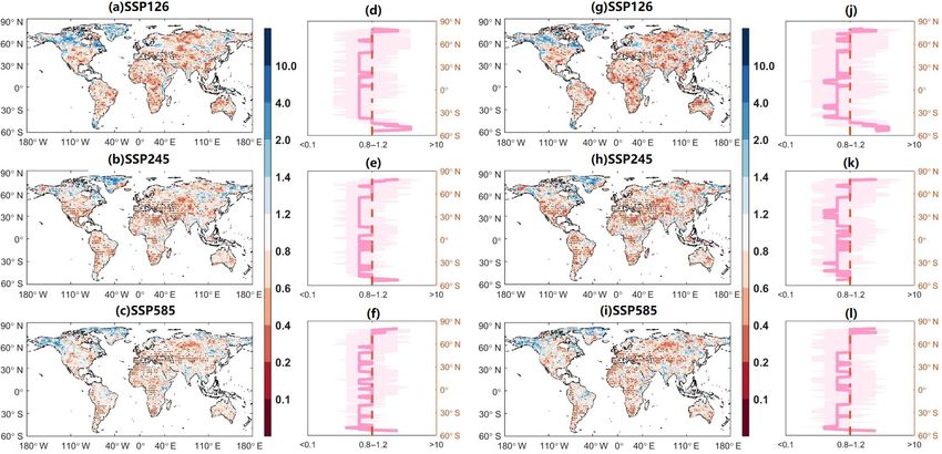
452                         L. Gu et al.: Projected increases in magnitude and socioeconomic exposure of global droughts

and references for mankind to enable appropriate adaptation         probably due to data constraint. These studies cannot cap-
strategies in a warmer future.                                      ture the dynamic nature of population and assets over time,
   To examine the sensitivity of drought risks with differ-         which has been identified as crucial for simulating realistic
ent warming targets, numerous approaches have emerged.              societal development paths (Smirnov et al., 2016). Recently,
One way is to employ a set of ensemble simulations pro-             five shared socioeconomic pathways (SSPs) have been pro-
duced by a single coupled climate model (e.g., Community            posed, providing a more reasonable dataset to characterize
Earth System Model, CESM) which is designed specifically            a set of plausible alternative futures of societal development
to perform the impact assessments at near-equilibrium sce-          with consideration of climate change and policy impacts over
narios of 1.5 or 2 ◦ C additional warming (Sanderson et al.,        the 21st century (Leimbach et al., 2017). To date, the SSPs
2017; Lehner et al., 2017). This single model type cannot           have not yet been incorporated into the drought impact as-
reflect the structural uncertainty of climate models, which         sessments with warming at the global scale.
is important in impact assessments, and thus raises doubts             More importantly, among existing global drought impact
about the robustness of such drought condition assessments          assessments, especially those targeting different warming
(Liu et al., 2018a). Emerging modeling efforts such as the          levels proposed by the Paris Agreement, drought variables
“Half a degree Additional warming, Projections, Prognosis           such as severity and duration are usually separately investi-
and Impacts” (HAPPI) model inter-comparison project pro-            gated through probability modeling and stochastic theories
vided a new dataset with experiments designed to explicitly         (e.g., Sanderson et al., 2017; Lehner et al., 2017; Su et al.,
target impacts of 1.5 and 2 ◦ C above preindustrial warming         2018). Knowing that droughts are multifaceted phenomena
(Mitchell et al., 2016). However, the HAPPI model employed          (Xu et al., 2015; Tsakiris et al., 2016) usually character-
prescribed climatological sea surface temperatures and could        ized by duration and severity, univariate frequency analysis
not consider the internal variability of ocean–atmosphere cir-      is unable to describe the probability of occurrence for the
culation, which is crucial in physically simulating climatic        drought events physically and may lead to underestimation
variability and persistence (Seager et al., 2005; Routson et        of drought risks and societal hazards. For instance, droughts
al., 2016). Current studies usually utilize CMIP5 climate           with a moderate severity but a long persistence are seldom
models to project climate scenarios under different repre-          identified as severe events in univariate analysis; neverthe-
sentative concentration pathways (RCPs), identify the time          less, they may pose substantial socioeconomic losses because
period for a warming target and then examine the drought            of rapid stored water depletion and low resilience to subse-
conditions associated with different levels of global warm-         quent droughts (Lehner et al., 2017). Therefore, there is an
ing. For instance, Su et al. (2018) used 13 CMIP5 mod-              urgent necessity to incorporate the joint modeling of mul-
els based on RCP2.6 and RCP4.5 to compare the drought               tiple drought features into impact assessments (Genest and
conditions for two warming targets over China and reported          Favre, 2007; Liu et al., 2015). The copula function that shows
that tremendous losses will emerge even under the ambitious         good feasibility of marginal distributions in modeling inter-
1.5 ◦ C warming target.                                             correlated variables has been introduced in multivariate anal-
   These prevailing tides of the literature almost reach a con-     ysis for droughts (e.g., Wong et al., 2013; Zhang et al., 2015;
sensus that, with a higher saturation threshold and more in-        Ayantobo et al., 2017). However, to the authors’ knowledge,
tense and frequent dry spells driven by rising temperatures,        no previous work links the high interdependence of drought
drought conditions would considerably worsen in many re-            characteristics to a global impact assessment under different
gions of the world (Mitchell et al., 2016; Liu et al., 2018a, b).   warming levels.
The potentially devastating impacts of more severe drought             In the multivariate framework, selection of variable com-
conditions on society raise considerable concerns, motivat-         binations along the quantile curve poses a new challenge,
ing a number of global socioeconomic assessments of future          as the choice of the joint return period (JRP) leads to in-
drought change impact (e.g., Below et al., 2007; Schilling et       finitely many such combinations. To meet the needs of infras-
al., 2012). For instance, Liu et al. (2018a) investigated global    tructure design and adaptivity, many researchers (e.g., Chen
drought evolution and corresponding population exposures            et al., 2010; Li et al., 2016; Zscheischler and Seneviratne,
in additional 1.5 and 2 ◦ C warming conditions using a set          2017) have assumed that the correlated variables have the
of CMIP5 models under RCP4.5 and RCP8.5. Naumann et                 same probability of occurrence under a given JRP, which is
al. (2018) assessed the development of drought conditions           called the equivalent frequency combination (EFC) method.
across the world for different warming targets in the Paris         Despite the fact that the EFC method has low calculation
Agreement. These studies concluded that there are consid-           complexity, the statistical and theoretical basis of the equal
erable benefits for the environment and society in limiting         frequency assumption is questionable (Yin et al., 2018a). To
warming to 1.5 ◦ C relative to 2.0 ◦ C, although 1.5 ◦ C warm-      develop a more rational design for a multivariate approach, a
ing still implies a substantial challenge for global sustain-       novel concept of “most likely design realization” to choose
able development. However, most previous socioeconomic              the point with the highest likelihood along the quantile curve
assessments (e.g., Peters, 2016; Park et al., 2018; Liu and         has been proposed in frequency analysis (Salvadori et al.
Sun, 2019) have focused on a static socioeconomic scenario,         2011; Yin et al., 2019a). It would be very important to eval-

Hydrol. Earth Syst. Sci., 24, 451–472, 2020                                        www.hydrol-earth-syst-sci.net/24/451/2020/
L. Gu et al.: Projected increases in magnitude and socioeconomic exposure of global droughts                                 453

uate and characterize these different likelihoods of drought      (Jones and O’Neill, 2016). Considering the socioeconomic
events in bivariate drought impact assessment under a warm-       challenges for mitigation along different development paths,
ing climate.                                                      the RCP2.6 scenario is associated with SSP1 (SSP126),
   In this study, under a bivariate framework, we quantify        which will face a lower challenge of mitigation in the fu-
changes in global drought conditions and socioeconomic ex-        ture. The RCP4.5 scenario is associated with SSP2 (SSP245),
posure with additional levels of 1.5 and 2.0 ◦ C warming.         while the highest emission scenario RCP8.5 is associated
The drought characteristics are identified using the Stan-        with SSP5 (SSP585), by which a relatively higher challenge
dardized Precipitation Evapotranspiration Index (SPEI) com-       is expected under foreseeable warming conditions (Samir
bined with the run theory and with climate scenarios sim-         and Lutz, 2017).
ulated by 13 CMIP5 global climate models (GCMs) un-
der three RCPs (RCP2.6, RCP4.5, and RCP8.5). The cop-             2.2     Definition of a baseline, 1.5 and 2 ◦ C global
ula functions and most likely realization are incorporated to             warming
model the drought severity and duration concurrently, and
changes in the bivariate return period with global warm-          The sensitivity of annual global temperature to climate vari-
ing are systematically investigated. Finally, the drought ex-     ability significantly varies in models and RCPs. Therefore,
posures of populations and regional gross domestic prod-          the time period with additional global warming of 1.5 and
uct (GDP) under different SSPs are assessed globally.             2 ◦ C with respect to preindustrial conditions also varies be-
                                                                  tween different climate scenarios. Here, the time periods
                                                                  for different global warming levels are determined using
                                                                  the 30-year running mean of a multi-model ensemble mean
2     Materials and method
                                                                  of global-mean surface air temperature, following previous
2.1    Climatic and socioeconomic scenarios                       studies (Vautard et al., 2014; Su et al., 2018). We first se-
                                                                  lect a baseline period of 1976–2005, during which the ob-
Climate projections are based on ensemble runs (r1i1p1) by        served global average temperature was approximately 0.46–
13 models from CMIP5 (Table 1), covering the period 1976–         0.66 ◦ C warmer than pre-industrial conditions (IPCC, 2018).
2100 under three RCPs (i.e., RCP2.6, RCP4.5, and RCP8.5).         This reference period is widely adopted for climate impact
   Ten climate variables were used in this study. Specifically,   assessment (e.g., Vautard et al., 2014), and we set the warm-
9 out of the 10 variables were applied for the calculation of     ing degree during the baseline period as 0.51 ◦ C; hence the
potential evapotranspiration (PET). These nine variables in-      1.5 and 2.0 ◦ C warming targets are determined by additional
clude surface maximum, mean, and minimum air tempera-             warming of 0.99 and 1.49 ◦ C, respectively. For each RCP, we
tures, surface wind speed, relative humidity, surface down-       define the 1.5 and 2 ◦ C warmer worlds by using the multi-
welling and upwelling longwave fluxes, and surface down-          model ensemble mean of global temperature. In other words,
welling and upwelling shortwave fluxes. The 10th variable         the reaching year is the same for all 13 GCMs under a spe-
is the precipitation. Then the calculated PET and GCM-            cific RCP scenario and is determined as the 30-year period
simulated precipitation were employed to calculate drought        with mean temperature closest to the warming target for each
indices. The PET was initially calculated at the daily scale.     RCP (see Fig. 1).
Then both the daily-scale PET and precipitation were aggre-
                                                                  2.3     Drought indices and event identification
gated to the monthly scales and bilinearly interpolated to a
spatial resolution of 1.0◦ × 1.0◦ on latitude and longitude for   2.3.1    Standardized Precipitation Evapotranspiration
each model simulation.                                                     Index
   To assess the exposures of populations and assets to
droughts, which will eventually lead to higher drought losses     The drought condition is quantified with the SPEI devel-
in the future, instead of using a static socioeconomic sce-       oped by Vicente-Serrano et al. (2010), which has been widely
nario as many studies have (e.g., Hirabayashi et al., 2013;       adopted in characterizing drought conditions (e.g., Ayantobo
Smirnov et al., 2016), we employ the spatially explicit global    et al., 2018; Wen et al., 2019). The SPEI quantifies the extent
shared SSPs. This dataset includes gridded population and         of atmospheric water surplus and deficit relative to the long-
GDP data under five SSPs, covering the period 2010–2100 at        term average condition by standardizing the difference be-
a spatial resolution of 0.5◦ × 0.5◦ (Jiang et al., 2017, 2018;    tween precipitation and potential evapotranspiration (PET).
Su et al., 2018; Huang et al., 2019). It involves a sustain-      The SPEI with a 3-month timescale (SPEI-3) is used in this
able scenario (SSP1), a pathway of continuing historical          study because it captures well the shallow soil moisture avail-
trends (SSP2), a strongly fragmented world (SSP3), a highly       able to crops and reflects seasonal water loss processes (Yu
unequal world (SSP4), and a growth-oriented world (SSP5).         et al., 2014).
Among combinations of different RCP trajectories and so-
cioeconomic pathways, some SSP–RCP combinations are
unlikely to occur, e.g., SSP3–RCP2.6 and SSP1–RCP8.5

www.hydrol-earth-syst-sci.net/24/451/2020/                                         Hydrol. Earth Syst. Sci., 24, 451–472, 2020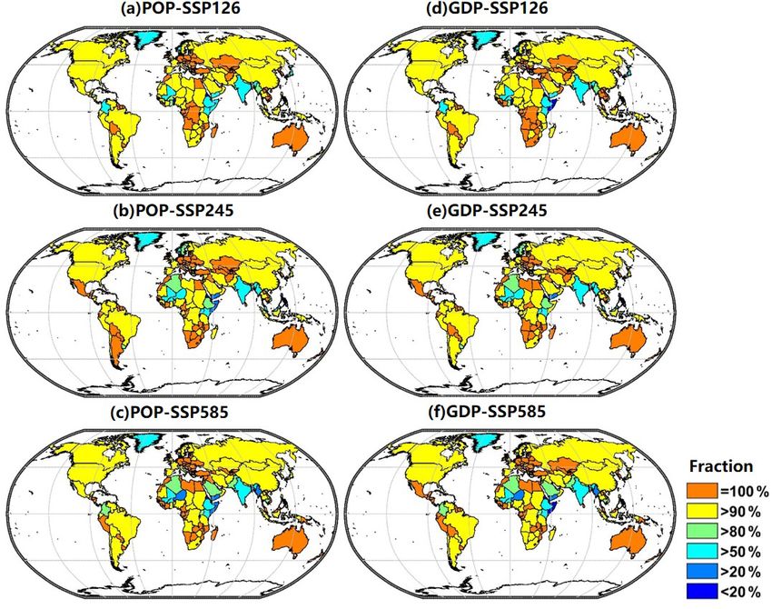
454                         L. Gu et al.: Projected increases in magnitude and socioeconomic exposure of global droughts

Table 1. Information about the 13 GCMs used in this study.

                     No.    Model name               Resolution   Institution
                                                                  College of Global Change and Earth System
                     1      BNU-ESM                   2.8 × 2.8
                                                                  Science, Beijing Normal University
                                                                  Canadian Centre for Climate Modelling and
                     2      CanESM2                   2.8 × 2.8
                                                                  Analysis
                                                                  Centre National de Recherches Météorologiques
                     3      CNRM-CM5                  1.4 × 1.4   and Centre Européen de Recherche et Formation
                                                                  Avancée en Calcul Scientifique
                                                                  Commonwealth Scientific and Industrial
                     4      CSIRO-Mk3.6.0             1.8 × 1.8   Research Organization and Queensland Climate
                                                                  Change Centre of Excellence
                     5      GFDL-CM3                  2.5 × 2.0
                     6      GFDL-ESM2G                2.5 × 2.0   NOAA Geophysical Fluid Dynamics Laboratory
                     7      GFDL-ESM2M                2.5 × 2.0
                     8      IPSL-CM5A-LR             3.75 × 1.9
                                                                  Institut Pierre Simon Laplace
                     9      IPSL-CM5A-MR             2.5 × 1.25
                     10     MIROC-ESM-CHEM            2.8 × 2.8   Japan Agency for Marine-Earth Science and
                     11     MIROC-ESM                 2.8 × 2.8   Technology, Atmosphere and Ocean Research
                                                                  Institute (University of Tokyo), and National
                                                                  Institute for Environmental Studies
                                                                  Atmosphere and Ocean Research Institute
                                                                  (University of Tokyo), National Institute for
                     12     MIROC5                    1.4 × 1.4
                                                                  Environmental Studies, and Japan Agency for
                                                                  Marine-Earth Science and Technology
                     13     MRI-CGCM3                 1.1 × 1.1   Meteorological Research Institute

                                                                         The PET is first calculated using the Penman–Monteith ap-
                                                                      proach suggested by the Food and Agriculture Organization
                                                                      of the United Nations (FAO) (Allen et al., 1998):
                                                                                0.4081 (Rn − G) + γ tmean900
                                                                                                          +273 u2 (es − ea )
                                                                      PET =                                                    ,   (1)
                                                                                           1 + γ (1 + 0.34u2 )
                                                                      where 1 is the slope of saturation vapor pressure vs. air tem-
                                                                      perature curve (kPa ◦ C−1 ) and is calculated by
                                                                                                  17.27×t−mean
                                                                                 0.6108 × e tmean +237.3
                                                                      1 = 4098 ×                         ,                         (2)
                                                                                     tmean + 237.3
                                                                      where tmean is the surface mean air temperature (◦ C). Rn is
                                                                      the net radiation (MJ m−2 d−1 ) and is calculated by
                                                                      Rn = [rsds − rsus − (rlus − rlds)] × 106 × 3600 × 24,        (3)
                                                                      where rsds and rsus (rlds and rlus) are surface downwelling
                                                                      and upwelling shortwave flux (surface downwelling and up-
                                                                      welling longwave flux), respectively (w m−2 ). G is the soil
Figure 1. Projected global mean temperatures when reaching            heat flux (MJ m−2 d−1 ) and is close to zero at the daily scale.
1.5 and 2.0 ◦ C warming.                                              γ is a psychometric constant (kPa ◦ C−1 ) and is calculated by
                                                                      γ = 0.665 × 10⁻³ × P ,                                       (4)

Hydrol. Earth Syst. Sci., 24, 451–472, 2020                                            www.hydrol-earth-syst-sci.net/24/451/2020/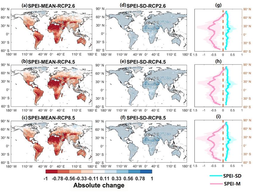
L. Gu et al.: Projected increases in magnitude and socioeconomic exposure of global droughts                                             455

where P is the atmospheric pressure (kPa). u2 is the wind          neglecting the multiplex nature of droughts (Naumann et al.,
speed at 2 m height (m s−1 ), transferred from                     2018). This study jointly models drought duration (D) and
                                                                   severity (S) via the copula function, which is versatile for
u2 = 4.87 × u10 / ln(67.8 × 10 − 5.42),                     (5)    describing dependent hydrological variables due to its good
where u10 is the surface wind speed at the 10 m height sim-        flexibility of marginal distributions. The widely used Gamma
ulated by GCMs. es and ea are saturation and actual vapor          distribution was adopted for fitting drought variables in each
pressure (kPa), respectively:                                      grid over the globe, and we selected the Gumbel copula to
                                                                   model the joint distribution of drought duration and severity.
                  17.27×tmp
                                                                   Within the copula-based approaches, different definitions of
es = 0.6108 × e tmp+237.3 ,                                 (6)
                                                                   joint return periods (JRPs) have been proposed, such as OR,
     RH                                                            AND, Kendall, dynamic, and structure-based return periods
ea =     × es ,                                             (7)
     100                                                           (Yin et al., 2019a). Among these, the OR case (Tor ) is usu-
where RH is the relative humidity (%) and tmp is temperature       ally adopted in drought occurrence assessment (Zhang et al.,
(i.e., daily maximum and minimum air temperature). Due to          2015):
the non-linearity of Eq. (6), it would be more appropriate to                  El               El
apply the average saturated vapor pressure derived from the        Tor =               =                       ,                        (10)
                                                                           1 − F (d, s) 1 − C [FD (d), FS (s)]
daily maximum and minimum air temperature.
   The widely used log-logistic distribution is employed           where El represents the expected inter-arrival time of
for fitting the 3-month deficit of precipitation and PET           drought events, the joint distribution F (d, s) could be de-
(P − PET) (Touma et al., 2015):                                    scribed by a copula function C[FD (d), FS (s)], and FD (d)
          "          β #−1                                       and FS (s) indicate the marginal distribution functions of D
                   α                                               and S, respectively.
F (x) = 1 +                   ,                           (8)
                 x −λ                                                 Under the bivariate framework, the choice of an appro-
                                                                   priate Tor leads to infinite combinations of drought duration
where F (x) denotes the cumulative distribution function;          and severity. The drought events along the Tor -level curve are
α, β and λ represent shape, scale and location parameters,         generally not equivalent in terms of environmental and soci-
which are estimated by the maximum likelihood method               etal consequences, and hence the likelihood of each event
(Ahmad et al., 1988).                                              must be taken into consideration when selecting appropri-
   The SPEI-3 can then be derived by standardizing the F (x)       ate joint quantiles. In this paper, the most likely realization
into a standard normal function with a transforming func-          method (Salvadori et al., 2011; Yin et al., 2019a) is used to
tion 8−1 as follows:                                               choose the drought scenario with the highest likelihood along
                                                                   the Tor -level isoline. For a given Tor , the most likely combi-
SPEI-3(x) = 8−1 (F (x)).                                    (9)    nation point among all possible events can be derived by the
2.3.2    Drought event identification                              following formula (Gräler et al., 2013):

                                                                       (d ∗ , s$∗ ) = argmaxf (d, s) = c [FD (d), FS (s)] fD (d)fS (s)
After calculating the SPEI-3 for global terrestrial grid cells,        C (FD (d), FS (s)) = 1 − El /Tor                                 , (11)
we derive the drought duration, intensity, and severity using
the run theory for the reference and the 1.5 and 2 ◦ C warmer      where f (d, s) represents the joint probability density func-
worlds. The run theory proposed by Yevjevich. (1967) is a          tion of drought duration and severity, c[FD (d), FS (s)] =
useful and objective method for drought event identification,      dC(FD (d), FS (s))/d(fD (d))d(fS (s)) indicates the density
where a run represents a subset of time series, in which SPEI-     function of the copula, and fD (d) and fS (s) are probability
3 is either beneath (i.e., negative run) or over (i.e., positive   density functions of drought duration and severity, respec-
run) a fixed threshold. A run with SPEI-3 that continuously        tively. Due to the complexity of deriving analytical solutions
stays below −0.5 is defined as a drought event (Mishra and         in Eq. (11), the harmonic mean Newton method (Yin et al.,
Singh, 2010; Zargar et al., 2011), which generally includes        2018a) is applied to estimate the most likely realizations.
drought characteristics of duration and severity. The persis-
tent time period during a drought event is further defined as      2.5     Calculation of socioeconomic exposure under
the drought duration, while drought severity (dimensionless)               warmer conditions
is defined as a cumulative deficit below −0.5.
                                                                   To calculate the socioeconomic exposures by droughts in
2.4     Bivariate return period and most likely realization        different warming environments, we evaluate the change in
        method                                                     drought occurrence frequency in a bivariate context. Firstly,
                                                                   we estimate the bivariate quantiles of drought duration and
Previous studies usually independently examined the change         severity (i.e., most likely realization) under one given JRP
either in drought duration or severity under climate warming,      during the historical period. As the 50-year drought events

www.hydrol-earth-syst-sci.net/24/451/2020/                                            Hydrol. Earth Syst. Sci., 24, 451–472, 2020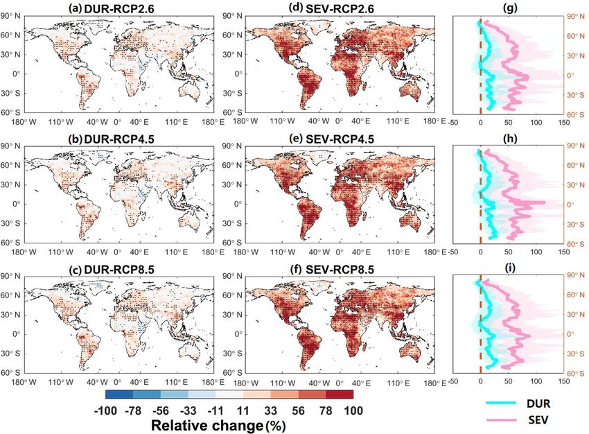
456                        L. Gu et al.: Projected increases in magnitude and socioeconomic exposure of global droughts

usually gained great attention by the scientific community       lower values and hence more severe dryness. Particularly,
and socio-climatic policymakers (Zhang et al., 2015; Nau-        dramatic decreases combined with strong model agreement
mann et al., 2018), we adopt this level as a reference for       (in terms of sign of change) are presented in South Amer-
assessing possible drought implications. With the historical     ica, Australia, and northern Africa. This may be attributed
50-year bivariate quantiles, we can recalculate the joint oc-    to higher evaporative demands and more frequent and persis-
currence frequency under future additional 1.5 and 2.0 ◦ C       tent dry spells associated with rising temperatures (Naumann
warming conditions, respectively. It can be inferred that ar-    et al., 2018). On the other hand, we also observe an increase
eas with a JRP lower than 50 years are projected to suffer       in the standard deviation of SPEI-3 with additional 1.5 ◦ C
from more severe drought conditions. To explicitly assess        warming, particularly in northern Africa and southwestern
the drought risk changes from 1.5 to 2.0 ◦ C warming cli-        Asia. As the SPEI-3 follows the standard normal distribu-
mates, we estimate the ratio of the recalculated recurrence      tion, the increasing standard deviation means more variabil-
frequency between these two warming periods. Taking the          ity in dryness, which hinders resilience efforts in a 1.5 ◦ C
50-year drought events as an example, we first determine the     warmer world. These changes are consistent under three dif-
magnitudes (duration and severity) of the 50-year drought        ferent RCPs, indicating the robustness of this globally drier
events in the historical period. Then we input the determined    future.
magnitudes of the 50-year drought events into the future joint      How would the dryness pattern change from 1.5 to 2.0 ◦ C
distribution functions, recalculate the joint recurrence fre-    warming climates? A progressive descending change in
quencies and convert them into new return periods at the         mean values of SPEI-3 is observed across 58 % of the land
1.5 and 2.0 ◦ C warming climates. The ratio is then calculated   surface with the global mean temperature increasing be-
by dividing the new return period in the 2.0 ◦ C warming fu-     tween 1.5 and 2.0 ◦ C, although several high-latitude regions
ture by the new return period in the 1.5 ◦ C warming. A ratio    (i.e., Russia, Canada) show an insignificant opposite change
less than 1.0 suggests that the new return period in 2.0 ◦ C     (Fig. 3). This may be mechanically explained by thick clouds
warming climates further reduces compared to that in the         in these regions that strengthen the reflectance of shortwave
1.5 ◦ C warming level, which means that reference drought        radiation and limit the increase in latent heat flux as well
events are more common under the 0.5 ◦ C warming impacts         as evapotranspiration, thus contributing to the mitigation of
and implies worrisome conditions.                                atmospheric aridity (Huang et al., 2017). For the change in
   To evaluate socioeconomic implications of drought with        the standard deviation of SPEI-3, we find that increases oc-
additional warming, we record the population and GDP in          cur over continental regions almost globally, accompanied by
those areas with more severe drought conditions and define       minor spatial variability. Overall, the climatic metric SPEI-
them as exposures by increasing drought risks. As previously     3 shows a strong negative response to the warming climate,
stated, we consider the dynamic nature of socioeconomic de-      suggesting that dryness will intensify in a future warming
velopment pathways by employing different SSPs and used          world.
the multi-year average populations and GDPs during 30-year
periods determined by different warming levels. After esti-
                                                                 3.2   Projected changes in drought characteristics
mating the socioeconomic exposures for each GCM simula-
tion, we use the multi-model ensemble mean as an indication
for each grid cell to reduce model bias. Note that we select     Figure 4 shows the relative change in global drought dura-
three RCPs and corresponding SSPs under two warming tar-         tion and severity derived from SPEI-3 in the 1.5 ◦ C warmer
gets so that the analysis is performed on six scenarios.         world relative to the historical period under three different
                                                                 RCPs. The drought duration is projected to slowly prolong
                                                                 with warming across 78 % of the land surface, and 44% of
3     Results                                                    land areas have an increase of higher than 10 %, although
                                                                 the change is not significant in the Russian and Sahel areas.
3.1    Projected changes in dryness                              The drought severity shows a much more pronounced rise
                                                                 globally, with significant increases (exceeding 50 %) over
We first examine changes in the mean and standard devia-         46 % of global landmasses. Moreover, several regions expe-
tion of SPEI-3 from the historical reference period (1976–       rience compound increases (with strong model agreement) in
2005) to the 1.5 ◦ C warmer worlds (Fig. 2), indicated by        both drought severity and duration, such as Southeast Asia,
the multi-model ensemble mean results. We find that mean         the Mediterranean, southern Africa, southern North America,
SPEI-3 decreases at the global scale (across 85 % of the land    and South America, suggesting an urgent need to increase
areas, excluding Antarctica), except in very limited regions     societal and environmental resilience to a warming climate
in high-latitude areas (e.g., Siberia in Russia), where it ex-   there. In the tropics and high-latitude areas, the drought
hibits a slight increase. The descending changes in the mean     severity is projected to increase, while the duration will de-
SPEI-3 imply that, over the majority of the globe, the prob-     crease. In these regions, mitigation strategies should target
ability distribution function of SPEI-3 would shift towards      short, intense bursts of drought.

Hydrol. Earth Syst. Sci., 24, 451–472, 2020                                    www.hydrol-earth-syst-sci.net/24/451/2020/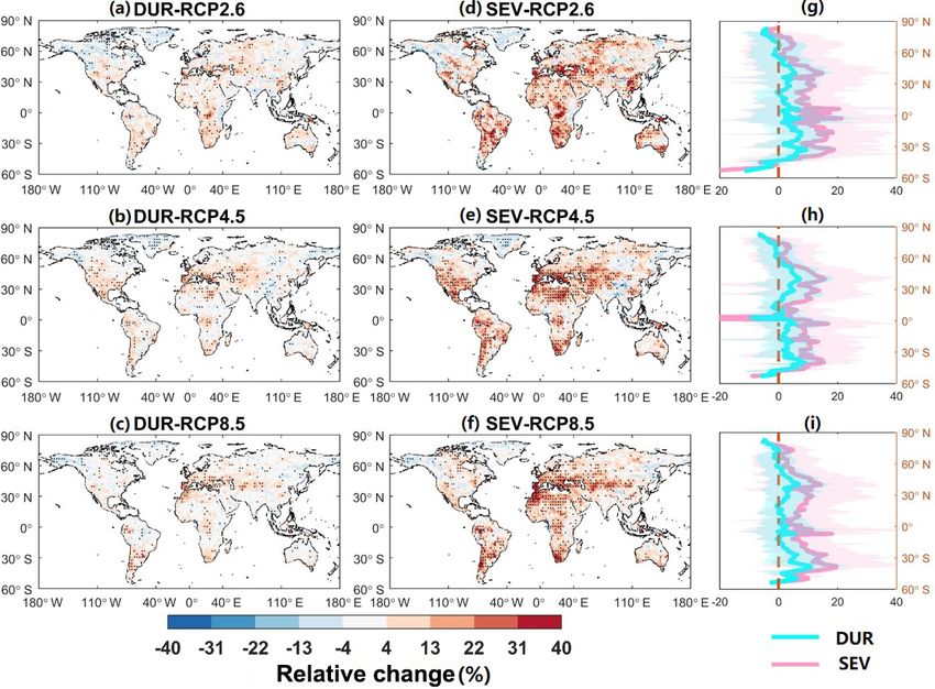
L. Gu et al.: Projected increases in magnitude and socioeconomic exposure of global droughts                                     457

Figure 2. Projected changes in the mean and standard deviation of the SPEI under the 1.5 ◦ C warming target.

   When the global temperature rises from additional 1.5 to               To explicitly investigate the changes in drought charac-
2.0 ◦ C warming, the world will experience more severe                 teristics under warming conditions, we also show statistics
drought conditions, with a further increase in drought sever-          of drought frequency, duration and severity in the historical
ity accounting for 75 % of the land surface (differences in            period and future additional warmer worlds in violin plots
effects between the 1.5 and 2.0 ◦ C warming levels) and a per-         (Fig. 6), in which the distributions comprise drought char-
sistent lengthening in duration across 58 % of the land areas          acteristics across all land pixels of the multi-model ensem-
(Fig. 5). Similar to the changing pattern from the baseline            ble mean results. The violin plots (Hintze and Nelson, 1998)
to a 1.5 ◦ C warming climate, the drought severity shows a             consist of a boxplot inside and an outside violin shape which
more rapidly increasing rate than drought duration globally            displays the probability distribution of drought characteris-
under the 2.0 ◦ C warming world. Comparing the 2.0 ◦ C to              tics. Apparently, the drought frequency based on SPEI-3 is
the 1.5 ◦ C warming condition, the increase in drought sever-          also projected to pronouncedly lengthen under three RCPs,
ity is greater than 10 % over 35 % of the land areas, while            accompanied by large variability capturing by the kernel den-
only 8 % of the land areas show such an increase (> 10 %) in           sity estimation in Fig. 6. This rapid increasing tendency also
drought duration. This drought-prone condition is more se-             holds true for drought duration and severity, and extreme
vere in several regions such as Mediterranean regions, South           conditions are projected to occur more frequently under
Africa and South America, posing large challenges for exist-           warming climates. For example, the 90 % uncertainty range
ing socio-hydrological systems there.                                  of drought duration (severity) increases from 2.2–6.5 to 1.8–
                                                                       7.8 months (from 2.1–6.6 to 2.0–12) under the 2.0 ◦ C warm-
                                                                       ing climate relative to the historical period.

www.hydrol-earth-syst-sci.net/24/451/2020/                                              Hydrol. Earth Syst. Sci., 24, 451–472, 2020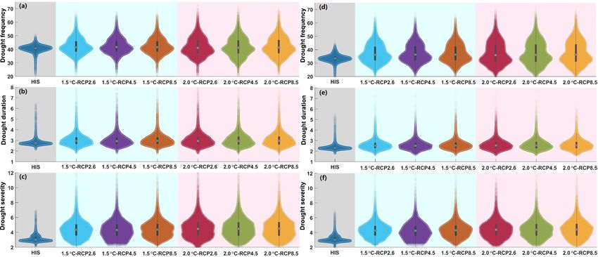
458 L. Gu et al.: Projected increases in magnitude and socioeconomic exposure of global droughts
Figure 3. Projected changes in the mean and standard deviation of the SPEI between the 1.5 and 2.0 ◦ C warming targets.
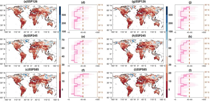
3.3 Projected changes in drought risks under the ambitious 1.5 ◦ C warming level. Regions with a
lower frequency of historical 50-year drought events indi-
cate a reduction in drought risks, which are only limited in
As evidence is accumulating that high-impact events are typ-
Siberia, the Indian peninsula, and Alaska.
ically multivariate in nature (Zhang et al., 2015; Ayantobo
To closely assess the drought conditions with an extra
et al., 2017), we now consider a deeper focus on changes in
0.5 ◦ C warming, we derive the ratio of an adjusted 50-year re-
drought severity and duration within a bivariate framework
turn period between 2.0 and 1.5 ◦ C warming worlds (Fig. 8).
under different warming levels. Using the copula-based ap-
In regions with a ratio of less than 1.0, the present drought
proach in Sect. 2.4, we show the median projected change in
events are projected to occur more frequently under the half-
the historical 50-year drought conditions over multi-model
degree additional warming, which accounts for 71 % of con-
ensembles under a 1.5 ◦ C warming climate (Fig. 7). Gen-
tinental areas. In addition, the frequency of the historical
erally, in regions with a substantial increase in drought du-
50-year droughts would double across 67 % of the global
ration and severity (Fig. 5), the 50-year drought events ex-
landmasses under the 2.0 ◦ C warming level. That is, 9 % in-
hibit a rapid increase in occurrence with warming. More than
crease in the world land areas compares to the 1.5 ◦ C warm-
88 % of global landmasses will be subject to more frequent
ing level (i.e., 58 %). Although over some regions such as
historical 50-year droughts, and the frequency of such se-
northern Canada and East Asia, the occurrence of the ex-
vere droughts would double over 58 % of the global land
treme droughts will be less frequent to some degree, strong
surface. For most areas of South America (except for the
rises in recurrence frequency with warming are projected to
zone around the Equator), northeastern America, central and
dominate large parts of Europe, the southern United States,
western Asia, and Northwest China, the historical 50-year
droughts are projected to occur 2 to 10 times more frequently
Hydrol. Earth Syst. Sci., 24, 451–472, 2020 www.hydrol-earth-syst-sci.net/24/451/2020/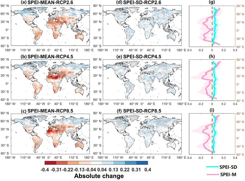
L. Gu et al.: Projected increases in magnitude and socioeconomic exposure of global droughts 459
Figure 4. Projected changes in drought duration and severity under the 1.5 ◦ C warming target.
Australia, South America, northern Africa, and the Mediter- Globally, three SSPs suggest a consistent projection that
ranean. large percentages of population and GDP will be exposed to
increasing drought risks. In more than 67 (140) countries,
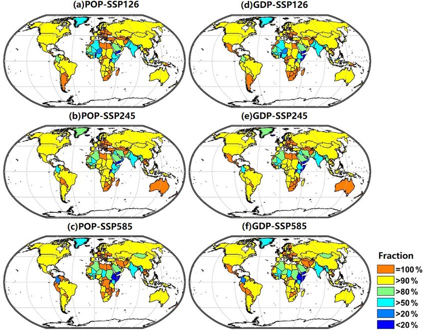
3.4 Population and GDP exposure from increasing 100 % (50 %) of both populations and GDPs are exposed
drought risks to more severe droughts under the 1.5 ◦ C warming target
(Fig. 9). The two socioeconomic factors of GDP and pop-
To understand the socioeconomic influences induced by in- ulation are highly correlated (O’Neill et al., 2014). Econom-
creasing drought risks (here defined as more frequent his- ically prosperous regions are associated with higher popu-
torical 50-year events), we combine the drought projection lation and immigration (Fig. S1 in the Supplement); thus,
with population and GDP information based on SSPs and es- the drought-affected GDP exposures usually exhibit simi-
timate exposures by droughts in the 1.5ãnd 2.0 ◦ C warmer lar changing patterns with the population. In regions with
worlds. Here, instead of using the absolute value of popula- low GDP and population density, even when total socioeco-
tion (and GDP) to assess the nation-wide drought exposures, nomic exposures to droughts seem small, droughts can still
the nation-wide population (and GDP) fraction is employed. cause fatal and destructive losses for those countries if their
This can avoid covering up badly drought-affected countries drought resilience is poor. To give a fairer and more impar-
where the national populations (or GDP) are small (or low) tial assessment of droughts’ socioeconomic consequences,
in terms of the world level. Specifically, for a country (e.g., we define and assess the fraction of drought-affected pop-
the United States), the fraction of drought-affected popula- ulation (or GDP) divided by total national population (or to-
tion (and GDP) divided by the total population (and GDP) of tal GDP) based on different countries in a 1.5 ◦ C warming
this country is employed as the indicator. Therefore, the most world. In addition, we see some interesting results. For ex-
drought-affected countries are presented by high fractions.
www.hydrol-earth-syst-sci.net/24/451/2020/ Hydrol. Earth Syst. Sci., 24, 451–472, 2020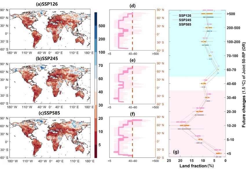
460                          L. Gu et al.: Projected increases in magnitude and socioeconomic exposure of global droughts

Figure 5. Projected changes in drought duration and severity between the 1.5 and 2.0 ◦ C warming targets.

ample, the US and China are no longer the most drought-                 ularly for the mitigation of population and GDP exposure
affected countries, while 100 % of the population and GDP               to drought. It should be noted that when climate warming
in the Mexico, southern Europe, central and southern Africa,            climbs from 1.5 to 2.0 ◦ C, there is some spatial heterogene-
and Mediterranean regions (i.e., Turkey, Ukraine) are pro-              ity with regards to drought exposure variations. Specifically,
jected to experience more severe drought, suggesting large              drought exposures for some countries (i.e., Canada) can be
policy challenges there.                                                slightly decreased in the 2 ◦ C warming level compared to
   To illustrate the consequences of limiting warming to                the 1.5 ◦ C warming level. This decrease in population and
2.0 ◦ C above the preindustrial levels, we also calculate the           GDP exposure fraction can be attributed to the decreasing
socioeconomic exposures under three SSPs (Fig. 10) and the              land fraction exposure to more frequent droughts (Table S2).
differences in percentage between the 1.5 and 2.0 ◦ C warm-             For example, the land fraction suffering more frequent se-
ing levels (Fig. S2). Most regions of the globe are projected           vere droughts in Canada will decrease (−12.77 %) in the
to exhibit a generally increasing fraction (relative to 1.5 ◦ C         2.0 ◦ C warming level compared to 1.5 ◦ C warming under
warming) in populations and GDPs (except for central Africa             the SSP126 scenario. In other words, the additional 0.5 ◦ C
and East Asia). To be specific, under the extra half-degree             warming will not lead to drought risk deterioration globally,
warming, an additional 17 countries are projected to exhibit            partly due to the increasing column-precipitable water with a
a 100 % fraction in socioeconomic exposure. More than 10                warming environment (Dong et al., 2019; Yin et al., 2019b),
countries would experience a 30 % increase in population                although it holds for the majority of global landmasses. Any-
and GDP exposure if the global warming level increased                  way, the spatial heterogeneity should be given attention, es-
from 1.5 to 2.0 ◦ C. These increases illustrate the benefit of          pecially when assessing the climate change impacts on ex-
holding global warming to 1.5 ◦ C instead of 2 ◦ C, partic-             treme events at regional or local scales (Liu et al., 2018b).

Hydrol. Earth Syst. Sci., 24, 451–472, 2020                                             www.hydrol-earth-syst-sci.net/24/451/2020/
L. Gu et al.: Projected increases in magnitude and socioeconomic exposure of global droughts                                         461

Figure 6. Distributions for drought characteristics under different time periods.

3.5   National assessment of socioeconomic exposure in                    aggregated changes explicitly show a significant increase in
      typical countries                                                   drought risks over these hotspot countries, with more than
                                                                          90 % of grid cells projected to suffer from more frequent
                                                                          droughts.
The large spatial variability of drought risks and socioeco-                 Nevertheless, we still observe a difference between the
nomic exposures under climate warming motivates a more                    tropics and extratropical regions. The increasing drought
systematic and in-depth assessment on national scales, par-               risks are more profound in tropical regions (e.g., Mexico
ticularly for the countries vulnerable to droughts. There-                and Brazil) than those over the high-latitude country (e.g.,
fore, we investigate more thoroughly the drought-affected                 Canada). For instance, in a 1.5 ◦ C warming world, more
land fractions (Figs. 11 and 12) and corresponding socioeco-              than 85 % of the grid cells (associated with around 65 %–
nomic exposure (Figs. S3 and S4) in eight hotspot countries               97 % of the national populations and GDPs) over Mexico and
spanning different socio-climatic regions: Argentina, Aus-                Brazil could be exposed to the historical 50-year drought ev-
tralia, Canada, China, United States, South Africa, Brazil,               ery 20 years. This pronounced increase in drought risks over
and Mexico.                                                               tropical countries may be attributed to an oceanic forcing that
   For assessment at the national scale, spatially aggregating            favors the formation of deep convection over the ocean and
mean changes are more helpful than per-grid cell changes                  thus weakened the continental convergence associated with
for indicating the risk of a particular land fraction being im-           the monsoon (Giannini et al., 2013). This finding suggests
pacted by climate change (Fischer et al., 2013; Lehner et                 that the tropics may confront more severe, frequent droughts
al., 2017). The land fractions of each grid cell are binned               and worse socioeconomic influences (Figs. S3 and S4) under
and plotted against the change in drought return period (rela-            a warming climate. When the additional warming target rises
tive to historical 50-year drought) (Figs. 11 and 12). The bin            up to 2.0 ◦ C, drought conditions worsen over all these exam-
number is fixed to 20 groups for the eight example coun-                  ple countries (Fig. 12). The increase in drought risks is still
tries. In a 1.5 ◦ C warming world (Fig. 11), these spatially

www.hydrol-earth-syst-sci.net/24/451/2020/                                               Hydrol. Earth Syst. Sci., 24, 451–472, 2020
462 L. Gu et al.: Projected increases in magnitude and socioeconomic exposure of global droughts
Figure 7. Projected changes in joint 50-year return periods of droughts under the 1.5 ◦ C warming target.
more pronounced in the tropical countries. More than 90 % spatial and decadal variability (Yin et al., 2018b). For global
of the grid cells (associated with around 90 %–100 % of the average precipitation, however, most climate models project
national population and GDP) across Brazil and Mexico will an increase of 1 %–3 % per degree warming (Liu et al., 2013).
experience drought frequency double that of the historical This deviation from the C–C relation law is due to a global ra-
50-year drought. diative energy constraint (Held and Soden, 2006) and atmo-
Overall, increasing drought risks under warming climates spheric moisture limitation by decreasing relative humidity
can cause major challenges for sustainable development and increasing the potential for intense tropical and subtropi-
and existing infrastructure systems, while ambitiously lim- cal thunderstorms under warming (Muller et al., 2011; Yin et
iting warming to 1.5 ◦ C would substantially mitigate future al., 2018b). Potential evapotranspiration, on the other hand,
drought risks and corresponding socioeconomic exposures. is predicted to increase by 1.5 %–4 % per degree warming
(Scheff and Frierson, 2014; Naumann et al., 2018). There-
fore, we expect climate warming to lead to a general inten-
4 Discussion sification of drought conditions, as the drying of the surface
is enhanced with water scarcity. This is confirmed by the de-
Among the warming-induced hydrological changes, one of creasing SPEI-3 and significantly increasing drought severity
the most definitive and detectable changes is the simultane- and duration with warming globally found here (Figs. 2–8).
ous increase in precipitation and evaporative demand, which The reference crop Penman–Monteith model is employed
are governed by the Clausius–Clapeyron relationship (Scheff to calculate potential evapotranspiration (and thus SPEI) in
and Frierson, 2014). Observations and model simulations the current study. In this process, surface resistance (rs ) is
have reported a variety of scaling rates between precipitation fixed to 70 s m−1 . However, according to recent studies (e.g.,
and global temperature, where the daily and hourly precipita- Roderick et al., 2015; Yang et al., 2019), an elevated CO2 en-
tion extremes (i.e., 99th/95th percentile precipitation) usually vironment can drive stomatal closure, increasing stomatal re-
exhibit a sub-C–C scaling at regional scales, accompanied by
Hydrol. Earth Syst. Sci., 24, 451–472, 2020 www.hydrol-earth-syst-sci.net/24/451/2020/L. Gu et al.: Projected increases in magnitude and socioeconomic exposure of global droughts 463
Figure 8. Projected changes in joint 50-year return periods of droughts between the 1.5 and 2.0 ◦ C warming targets.
sistance and further increasing rs . Subsequently, this increas- the other hand, different threshold values in identifying a
ing rs causes the decline in the potential evapotranspiration, drought event may cause disparities regarding drought risk
especially across vegetated lands where the photo-synthetic changes and may challenge the robustness of our results.
rate is high. From this perspective, the neglect of increas- Generally, the threshold value usually ranges between −1
ing rs may overestimate future drying conditions and corre- and 0 (Xu et al., 2015; Ayantobo et al., 2017, 2018; Yuan
sponding drought risk changes to some extent. However, on et al., 2017; Jiao and Yuan, 2019). Herein, the threshold
the other hand, the increase in total leaf area with CO2 and of −0.5 is employed to identify droughts varying from mild
growing-season length can cause countervailing decreases to extremely dry levels (Table 2, Chen et al., 2018), which
in rs (Greve et al., 2019). Overall, accurate and robust quan- has been widely adopted in drought-related studies (Liu and
tification of rs scaling with CO2 still needs additionally ex- Jiang, 2015; Xiao et al., 2017; Chen et al., 2018). The inclu-
plicit work and substantial observed data. Though the impact sion of minor drought events can enlarge the sample size in
of rs on the drought assessments deserves further studies, it bivariate frequency analysis and thus circumvents the prob-
is beyond the scope of this study. Therefore, the traditional lem of insufficient samples. Moreover, to verify the robust-
fixed rs method is used in this study to calculate potential ness of our results, we also use the −0.8 threshold to serve
evapotranspiration. as a comparison. Relevant results are shown in Figs. 13–15.
In the run theory, once the threshold (e.g., −0.5) is de- Figure 13 displays comparisons of distributions comprising
termined, drought events with different severity magnitudes drought characteristics (i.e., drought frequency, drought du-
are identified and constitute a sample for the selected time ration and drought severity) across all land pixels between
period. This sample contains different magnitudes in sever- using −0.8 and −0.5 as the thresholds. Figures 14 and 15
ity and different lengths in the duration, therefore character- show comparisons of projected changes in joint 50-year re-
izing the distribution of different levels of drought (rang- turn periods of droughts between using −0.8 and −0.5 as the
ing from the mild, moderate, to extreme conditions). On thresholds under different warming levels. As shown in the
www.hydrol-earth-syst-sci.net/24/451/2020/ Hydrol. Earth Syst. Sci., 24, 451–472, 2020464 L. Gu et al.: Projected increases in magnitude and socioeconomic exposure of global droughts Figure 9. National population and GDP fraction exposure to more frequent severe droughts under the 1.5 ◦ C warming target. Figure 10. National population and GDP fraction exposure to more frequent severe droughts under the 2.0 ◦ C warming target. Hydrol. Earth Syst. Sci., 24, 451–472, 2020 www.hydrol-earth-syst-sci.net/24/451/2020/
L. Gu et al.: Projected increases in magnitude and socioeconomic exposure of global droughts                                 465

Figure 11. Projected changes in drought risks for eight typical   Figure 12. Projected changes in drought risks for eight typical
drought-prone countries under the 1.5 ◦ C warming target.         drought-prone countries under the 2.0 ◦ C warming target.

                                                                  Table 2. Drought categories in the SPEI.
figure (Fig. 13), drought characteristics tend to slightly de-
crease across different periods. However, future drought risk
                                                                                 SPEI             Categories
changes as indicated by the 50-year joint return period de-
riving from the −0.8 threshold are similar to those from the                     > −0.5           Near normal
−0.5 threshold (Figs. 14 and 15). In addition, we also de-                       −1.0 to −0.5     Mild drought
rive changes in drought risks for the 20- or 100-year drought                    −2.0 to −1.0     Moderate drought
                                                                                 < −2.0           Extreme drought
events to explore risk variations caused by different extents
of drought (Figs. S5 and S6). Results show that although the
magnitudes of changes are different, they present quite simi-
lar spatial patterns. Furthermore, since the calculation of so-   jected changes generally display strong model agreement (in
cioeconomic exposures to droughts is based on the variations      terms of sign of change), which implies high confidence in
of drought risks when employing the same dynamic popu-            these drought-prone areas. Conversely, substantial model un-
lation (and GDP) pathways, similar changes in the drought         certainty of drought projections is particularly clear for re-
risks will lead to analogical socioeconomic exposures. As a       gions with small changing amplitudes, as indicated by weak
reference, we analyze the socioeconomic exposures in the          model agreement (e.g., Southeast Asia and Russia). For ex-
case when −0.8 is used as the threshold (Figs. S7 and S8).        ample, 100 % of the population in tropical regions like Brazil
Compared with the results of the −0.5 threshold (Figs. 9          and Mexico would be affected by increasing drought risks.
and 10), the overall characteristics of the drought exposures     Indeed, our finding that the tropical and mid-latitude regions,
are mostly the same. This confirms the conclusions of our         where the vast majority of the global population resides,
study.                                                            would bear the greatest drought risks should be precautious
   Although aggravated drought risks are projected glob-          under the foreseeable warming future. Previous studies have
ally, the changing patterns exhibit large spatial variabil-       reported that the increases in El Niño frequency (Xie et al.,
ity, with more significant increases over mid-latitudes and       2010), an extension of the Hadley cell (Lu et al., 2007), and
tropical regions than those over high-latitude landmasses.        poleward moisture transport by transient eddies (Chou et al.,
It should be noticed that regions (e.g., the Mediterranean,       2009) under warming all contribute to the drying tendency in
southern Africa, southern North America) with large pro-          the tropics; however, our work does not quantitatively exam-

www.hydrol-earth-syst-sci.net/24/451/2020/                                        Hydrol. Earth Syst. Sci., 24, 451–472, 2020
466 L. Gu et al.: Projected increases in magnitude and socioeconomic exposure of global droughts Figure 13. Distribution for drought characteristics when using −0.5 as the threshold and −0.8 as the threshold, respectively. Figure 14. Projected changes in joint 50-year return periods of droughts when using −0.5 as the threshold and −0.8 as the threshold under the 1.5 ◦ C warming target. ine these underlying physical mechanisms behind the spatial conomic impacts. This neglect may lead to biased conclu- variability due to paucity of data. sions. In this study, the dynamic characteristics are consid- When investigating socioeconomic exposure (i.e., popula- ered differences in population (and GDP) between the fixed tion and GDP) under different warming levels, we notice that 30-year 1.5 and 2.0 ◦ C warming periods (Table 3). Accord- drought risks and population (GDP) both contribute to the ingly, the exposure is defined as the number of people (GDP) exposure change. However, the use of population and GDP being exposed to areas where the bivariate drought risks in- for a single year (i.e., 2005 or 2100), which have been used crease under the warming climate. Under the 1.5 ◦ C warming by some earlier studies (e.g., Peters, 2016; Park et al., 2018; climate, there are around 88 % of global landmasses being Liu et al., 2018a), has ignored the role of dynamic socioe- exposed to increasing drought risks, which corresponds to Hydrol. Earth Syst. Sci., 24, 451–472, 2020 www.hydrol-earth-syst-sci.net/24/451/2020/
L. Gu et al.: Projected increases in magnitude and socioeconomic exposure of global droughts                                          467

Figure 15. Projected changes in joint 50-year return periods of droughts when using −0.5 as the threshold and −0.8 as the threshold between
the 1.5 and 2.0 ◦ C warming targets.

USD 1386.9 million population (and USD 33311.1 billion)                 Table 3. Global population and GDP in the 1.5 and 2.0 ◦ C warming
according to the average of the three SSPs from a global per-           climates.
spective. At the 2.0 ◦ C warming level, though there are still
88 % of the global land areas being exposed to increasing                                                 SSP126     SSP124     SSP585
drought risks, the affected population (and GDP) will soar                1.5 ◦ C population (million)      1516.9    1553.5     1510.8
to 1538.2 million (and USD 72852.2 billion). In this light,               2.0 ◦ C population (million)      1666.7    1731.2     1603.1
the increase in population (and GDP) contributes to the in-               1.5 ◦ C GDP (billion USD)       35 875.0   34 244.0   35 668.5
creasing exposures. Therefore, it is important to incorporate             2.0 ◦ C GDP (billion USD)      11 6991.1   56 271.6   58 916.2
the dynamic population (and GDP) into exposure-calculating
processes. Nevertheless, when further investigating the af-
fected population (and GDP) between the two warming cli-                by multi-model ensembles are quantified in each grid under
mates, the role of drought risk changes should also be given            three RCPs (Figs. S9 and S10). Compared with the ensem-
attention. Specifically, though the percentage of landmasses            ble mean change in SPEI-3 shown in Figs. 2 and 3, we find
with increasing drought risks stays unchanged for both the              that the model uncertainty is relatively large, particularly for
1.5 and 2.0 ◦ C warming climates (both approximately 88 %),             South America and Africa, where the 90 % range even ex-
the magnitudes of risk changes are different. For instance,             ceeds the ensemble mean change. This finding also holds true
drought risks will double across around 58 % of the global              when evaluating the drought duration and severity (Figs. S11
landmasses at the 1.5 ◦ C warming level, while the same                 and S12), suggesting that model uncertainty cannot be ig-
drought risks will occur over 67 % of the global landmasses             nored in climate change impact studies.
at the 2.0 ◦ C warming level. Those differences in the magni-              To fully consider model uncertainty on drought conditions,
tudes of drought risk changes can definitely bring about di-            we also present the bivariate return period of the present
vergent impacts to the local population and economy. There-             50-year drought condition for each model under RCP4.5 in
fore, our study strengthens the benefits and necessity of con-          a 1.5 ◦ C warming world and the occurrence change under
trolling the global warming at the 1.5 ◦ C level.                       an additional 0.5 ◦ C warming (Figs. S13 and S14). As ex-
   For a complete analysis of climate change impact assess-             pected, different climate models show large variations, and
ment, it is important to know the role of corresponding un-             several models even exhibit opposite changes over certain re-
certainty especially induced by GCMs and RCP scenarios.                 gions. Despite this uncertainty, most models still project gen-
Measured by the 90 % range of the changing characteris-                 eral increasing risks at the global scale under climate warm-
tics of SPEI-3 from historical to 1.5 ◦ C warming worlds and            ing, particularly for mid-latitude areas and the tropics. For
from 1.5 to 2.0 ◦ C warming targets, the uncertainties induced          RCP uncertainty, although we notice that the three scenarios

www.hydrol-earth-syst-sci.net/24/451/2020/                                               Hydrol. Earth Syst. Sci., 24, 451–472, 2020
You can also read