X-band dual-polarization radar-based hydrometeor classification for Brazilian tropical precipitation systems
←
→
Page content transcription
If your browser does not render page correctly, please read the page content below
Atmos. Meas. Tech., 12, 811–837, 2019
https://doi.org/10.5194/amt-12-811-2019
© Author(s) 2019. This work is distributed under
the Creative Commons Attribution 4.0 License.

X-band dual-polarization radar-based hydrometeor classification
for Brazilian tropical precipitation systems
Jean-François Ribaud, Luiz Augusto Toledo Machado, and Thiago Biscaro
National Institute of Space Research (INPE), Center for Weather Forecast and Climate Studies (CPTEC),
Rodovia Presidente Dutra, km 40, Cachoeira Paulista, SP, 12 630-000, Brazil

Correspondence: Jean-François Ribaud (jean-francois.ribaud@inpe.br)

Received: 25 May 2018 – Discussion started: 19 September 2018
Revised: 22 December 2018 – Accepted: 14 January 2019 – Published: 6 February 2019

Abstract. The dominant hydrometeor types associated with           1   Introduction
Brazilian tropical precipitation systems are identified via re-
search X-band dual-polarization radar deployed in the vicin-       The use of dual-polarization (DPOL) radars over several
ity of the Manaus region (Amazonas) during both the GoA-           decades by national weather services as well as research lab-
mazon2014/5 and ACRIDICON-CHUVA field experiments.                 oratories has deeply changed the understanding and forecast-
The present study is based on an agglomerative hierarchical        ing of many precipitation events around the world. By us-
clustering (AHC) approach that makes use of dual polarimet-        ing a second orthogonal polarization, such weather radars
ric radar observables (reflectivity at horizontal polarization     enable inference of the size, shape, orientation, and phase
ZH , differential reflectivity ZDR , specific differential-phase   state of different particles detected within the sampled cloud.
KDP , and correlation coefficient ρHV ) and temperature data       To date, the major advances that have been made as a re-
inferred from sounding balloons. The sensitivity of the ag-        sult of DPOL radar sensitivities are mainly related to im-
glomerative clustering scheme for measuring the interclus-         provement in the distinction between meteorological and
ter dissimilarities (linkage criterion) is evaluated through the   non-meteorological echoes, attenuation correction, quantita-
wet-season dataset. Both the weighted and Ward linkages ex-        tive rainfall estimation, and bulk hydrometeor classification
hibit better abilities to retrieve cloud microphysical species,    (Bringi and Chandrasekar, 2001; Bringi et al., 2007). By
whereas clustering outputs associated with the centroid link-      combining DPOL radar observables (generally, reflectivity
age are poorly defined. The AHC method is then applied to          at horizontal polarization, ZH ; differential reflectivity, ZDR ;
investigate the microphysical structure of both the wet and        specific differential phase, KDP ; and correlation coefficient,
dry seasons. The stratiform regions are composed of five hy-       ρHV ) with some extra information such as temperature to lo-
drometeor classes: drizzle, rain, wet snow, aggregates, and        cate the freezing level, the hydrometeor identification task
ice crystals, whereas convective echoes are generally associ-      has been the subject of many research studies. Indeed, po-
ated with light rain, moderate rain, heavy rain, graupel, ag-      tential benefits from this research topic are numerous such
gregates, and ice crystals. The main discrepancy between the       as the evaluation of microphysical parameterization in high-
wet and dry seasons is the presence of both low- and high-         resolution numerical weather prediction models (e.g. Augros
density graupel within convective regions, whereas the rainy       et al., 2016; Wolfensberger and Berne, 2018), investigation
period exhibits only one type of graupel. Finally, aggregate       of relationships between microphysics and lightning (e.g.
and ice crystal hydrometeors in the tropics are found to ex-       Ribaud et al., 2016a), and improvement in weather nowcast-
hibit higher polarimetric values compared to those at midlat-      ing for high-impact meteorological events (hailstorms, flight
itudes.                                                            assistance, and road safety).
                                                                      Three hydrometeor classification schemes have been de-
                                                                   veloped since the emergence of DPOL radar in the 1980s:
                                                                   (1) supervised, (2) unsupervised, and (3) semi-supervised
                                                                   techniques (Fig. 1).

Published by Copernicus Publications on behalf of the European Geosciences Union.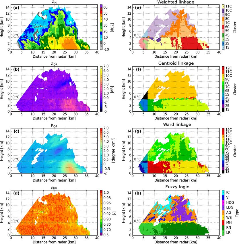
812                                     J.-F. Ribaud et al.: X-band dual-polarization radar-based hydrometeor classification

Figure 1. Schematic representation of the different hydrometeor classification techniques and their principal associated benchmarks.

  1. The supervised method constitutes, by far, most of                           sets of non-linear radar data into scalar outputs re-
     the literature and is subdivided into three different                        ferring to different microphysical species. In this re-
     techniques: the Boolean tree method, fuzzy logic, and                        gard, each hydrometeor-type distribution is charac-
     the Bayesian approach. Here, the supervised technique                        terized by a membership function coming from ei-
     refers to a priori and arbitrarily identified hydrometeor                    ther T-matrix simulations (Mishchenko and Travis,
     types from which DPOL radar responses have been de-                          1998) or, less frequently, aircraft in situ measure-
     rived from either theoretical models or empirical knowl-                     ments. The hydrometeor inference is finally the re-
     edge. Polarimetric observations are then assigned to the                     sult of a combination of membership functions and
     most suitable hydrometeor types according to their sim-                      a set of a priori rules defined by the user (Straka,
     ilarities.                                                                   1996; Vivekanandan et al., 1999; Liu and Chan-
                                                                                  drasekar, 2000; Marzano et al., 2006; Park et al.,
       – Boolean method. This technique is the easiest way                        2009; Dolan and Rutledge, 2009; Al-Sakka et al.,
         to identify dominant hydrometeor populations and                         2013; Thompson et al., 2014). This method is rela-
         has consequently been the first to be used. The                          tively simple to implement and computationally in-
         algorithm relies on the beforehand definition of                         expensive. A few studies, such as the Joint Polar-
         the ranges of DPOL radar-observable values for                           ization Experiment (Ryzhkov et al., 2005) for hail
         each hydrometeor type by the user. Then, a simple                        detection or even the recent use of a fuzzy-logic al-
         Boolean decision is applied to retrieve the dominant                     gorithm as an operational tool for national weather
         hydrometeor type (Seliga and Bringi, 1976; Hall                          services (Al-Sakka et al., 2013), have demonstrated
         et al., 1984; Bringi et al., 1986; Straka and Zrnić,                    the robustness of this hydrometeor classification al-
         1993; Höller et al., 1994). This approach, neverthe-                     gorithm type in singular environments.
         less, does not take into account the fact that differ-
                                                                                – Bayesian approach. In this case, the hydrometeor
         ent hydrometeor types can be defined on the same
                                                                                  identification task is expressed in a probabilistic
         range of values for the same polarimetric radar ob-
                                                                                  form based on synthetic data derived from polari-
         servable and, therefore, frequently leads to misclas-
                                                                                  metric radar simulation of different hydrometeor
         sification.
                                                                                  types (with each one being characterized by a cen-
       – Fuzzy-logic technique (Mendel, 1995). This super-                        tre and a covariance matrix). The final supervised
         vised algorithm type fixed the previous limitation                       hydrometeor inference is then performed by adapt-
         by allowing a smooth transition of DPOL radar-                           ing the maximum a posteriori rule. Another inter-
         observable ranges for all hydrometeor types. The                         esting attribute of the Bayesian technique resides in
         originality of fuzzy logic is its ability to transform                   the appealing possibility of retrieving the liquid wa-

Atmos. Meas. Tech., 12, 811–837, 2019                                                        www.atmos-meas-tech.net/12/811/2019/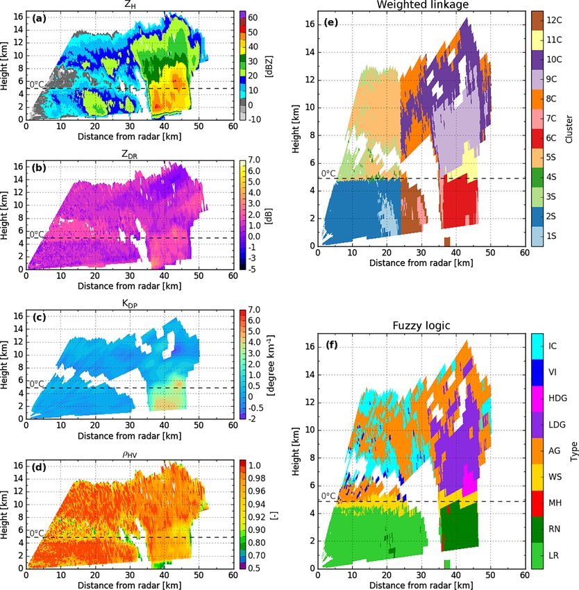
J.-F. Ribaud et al.: X-band dual-polarization radar-based hydrometeor classification                                             813

          ter content associated with each hydrometeor type          initially developed for S-band radar before being adapted to
          (Marzano et al., 2008, 2010).                              both C- and X-band radars, and research studies have largely
                                                                     been done in North America, Europe, and Oceania.
  2. More recently, Grazioli et al. (2015), or even Grazi-               The present study aims to develop the first HCA for
     oli et al. (2017), proposed an innovative unsupervised          Brazilian tropical precipitation systems via an X-band dual-
     approach to identifying the dominant hydrometeor dis-           polarization radar used in both the GoAmazon2014/5 and
     tribution within precipitation events, where hydrome-           ACRIDICON-CHUVA field experiments (Martin et al.,
     teor types are retrieved by gathering observable simi-          2016, 2017; Wendisch et al., 2016; Machado et al., 2018).
     larities in DPOL radar data. Indeed, the unsupervised           Although the area constitutes an intriguing location with both
     technique refers to a set of unlabelled data observations       a high amount of rain and complex aerosol–cloud interaction
     for which the goal is to group them into clusters shar-         (e.g. Cecchini et al., 2017; Machado et al., 2018), there are al-
     ing similar properties based on innate structures of the        most no references for hydrometeor classification over trop-
     data (variance, distribution, etc.) and without using a         ical land, especially for the Amazon region. In this regard,
     priori knowledge. To achieve this goal, the authors used        the studies by Dolan et al. (2013) and Cazenave et al. (2016)
     an agglomerative hierarchical clustering technique to-          took place in singular locations (Darwin, Australia, and Ni-
     gether with a spatial constraint on the consistency of          amey, Niger, respectively). These studies used a supervised
     the classification (homogeneity). This data-driven ap-          fuzzy logic approach to retrieve the hydrometeor distribu-
     proach mainly avoids the numerical-scattering simula-           tion within precipitation events with a C- and adapted X-
     tions used in fuzzy logic, which are well designed for          band scheme, respectively. As aforementioned, fuzzy-logic
     the liquid phase but questionable for ice-phase micro-          algorithms use weights to constrain the final identification.
     physics. Finally, interpretation of the clusters (labelling)    Another issue that might be related to hydrometeor identi-
     is done manually.                                               fication tasks is the use of the melting layer as a parameter
  3. Although initially mentioned by Liu and Chandrasekar            to detect liquid-ice delineation. However, liquid water above
     (2000), the first complete study based on a semi-               the melting layer within the convective tower of tropical sys-
     supervised approach was done by Bechini and Chan-               tems is not unusual (Cecchini et al., 2017; Jäkel et al., 2017).
     drasekar (2015), recently followed by the works of Wen          For instance, Cecchini et al. (2017) retrieved liquid water at
     et al. (2015, 2016) and Besic et al. (2016). This tech-         as low as −18 ◦ C within polluted tropical convective clouds.
     nique combines the advantages of the fuzzy logic and            Classification using cluster analysis allows the use of natu-
     clustering methods. The algorithm initially begins with         ral (non-imposed) classes of ice-water species. For all these
     a fuzzy-logic classification, which is then adjusted by         reasons, the present paper deals with the first unsupervised
     a K-means clustering method that iteratively allows for         clustering method based on X-band DPOL radar measure-
     rectifying the initial membership function of each hy-          ments in the Brazilian tropical region. Three main questions
     drometeor type according to the observed DPOL radar             are addressed in this paper. (1) What is the sensitivity of the
     measurements. In addition, constraints such as temper-          clustering algorithm to the different linkage methods, and
     ature limits and/or spatial distribution can be imple-          how can one improve the liquid–solid delineation? (2) What
     mented in this self-adapting methodology.                       are the hydrometeor classification output characteristics for
                                                                     both wet and dry tropical seasons in Amazonas? (3) What
Overall, these hydrometeor classification algorithms (HCAs)          are the microphysical distribution differences within tropical
still require in situ aircraft validations (especially within con-   convective and stratiform cloud systems between the wet and
vective cores) that are problematic due to their cost and, ob-       dry seasons?
viously, the danger of obtaining such measurements. Only                 The article is organized as follows: Sect. 2 provides a brief
a few studies have had the opportunity to use limited air-           description of the radar dataset, while Sect. 3 presents the
craft measurements and generally compared a few isolated in          AHC method. The sensitivity of the AHC to the linkage
situ images with HCA outputs (Aydin et al., 1986; El-Magd            methods together with a potential temperature improvement
et al., 2000; Cazenave et al., 2016; Ribaud et al., 2016b).          is assessed and discussed in Sect. 4. The hydrometeor iden-
Another limitation of these studies using methods such as            tification for Brazilian tropical system events is presented in
the fuzzy-logic approach is the dependency of their valid-           terms of wet–dry seasons and stratiform–convective regions
ity, since they are generally both wavelength- and climati-          in Sect. 5, while a discussion of hydrometeor distribution
cally radar-dependent. Although T-matrix simulations for a           comparisons is presented in Sect. 6.
radar wavelength have been theoretically demonstrated, each
final algorithm is then tuned by giving weights to each DPOL
radar observable to allow them to fit as closely as possible         2   Datasets and processing
with local ground observations. Finally, one can also see that
the related hydrometeor identification literature is mainly          The data used in this study are mainly based on DPOL
concerned with the midlatitudes. Indeed, the methods were            radar data observations collected during both the GoAma-

www.atmos-meas-tech.net/12/811/2019/                                                      Atmos. Meas. Tech., 12, 811–837, 2019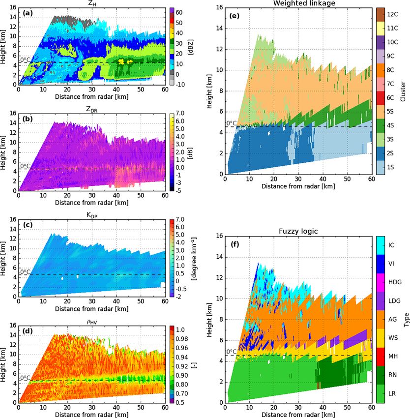
814                                  J.-F. Ribaud et al.: X-band dual-polarization radar-based hydrometeor classification

Figure 2. (a) Geographical localization of the GoAmazon2014/5 and ACRIDICON-CHUVA experiments. (b) X-band DPOL radar coverage
and its associated topography.

zon2014/5 and ACRIDICON-CHUVA experiments that took               four-step process has been applied to the DPOL radar dataset
place around the city of Manaus in the Amazonas state of          which consists of (i) calibration of ZDR , (ii) identification
Brazil (Fig. 2). Both of these research experiments aimed to      of meteorological and non-meteorological echoes, (iii) 8DP
investigate the complex mechanisms at play within tropical        filtering and estimation of the derivative specific differential-
weather through intriguing interactions between human ac-         phase KDP (Hubbert and Bringi, 1995), and (iv) attenuation
tivities and the neighbouring tropical forested region. In this   correction applied to both ZH and ZDR based on the ZPHI
regard, the present study considers the wet and dry seasons       method proposed by Testud et al. (2000). The calibration of
as corresponding to the intensive operating periods (IOPs) of     ZDR has been adjusted by using vertically pointing scans
the GoAmazon2014/5 field experiment (Martin et al., 2016),        for cases with no rain attenuation (drizzle/light rain). This
which were from 1 February to 31 March 2014 (wet sea-             method allows the ZDR offset to be temporally calculated
son: 59 days) and 15 August to 12 October 2014 (dry season:       since 0 dB is expected. The offset has been then removed in
60 days).                                                         subsequent ZDR measurements. A second analysis of ZDR
   Among all the instruments deployed, a SELEX Gema-              was occasionally realized by checking ZDR values within a
tronik X-band DPOL radar was located in the city of Man-          stratiform light-rain medium and characterized by ZH values
acapuru in 2014 to complete the radar coverage from the           between 20 and 22 dBZ. The expected ZDR value was 0.2 dB
Manaus Doppler radar, as well as to provide more micro-           as shown by Illingworth and Blackman (2002) or Segond
physical details about the South American monsoon meteo-          et al. (2007). Note that the dataset has also been restricted
rological systems (Oliveira et al., 2016). The X-band DPOL        to precipitation events wherein the radome of the X-band
radar was operated at 9.345 GHz with a 1.3◦ beam width            DPOL radar was dry in order to remove any additional at-
at −3 dB and in simultaneous transmission and reception           tenuation (Bechini et al., 2010). In addition to these consid-
(STAR) mode (Schneebeli et al., 2012; and Table 1). The           erations, a signal-to-noise ratio of SNR ≥ +10 dB as well
latter characteristic allows the reflectivity to be obtained      as a reduced radar coverage ranging from 5 to 60 km, have
at horizontal polarization ZH , differential reflectivity ZDR ,   been considered for this study to mitigate potential remain-
differential-phase 8DP , and correlation coefficient ρHV . The    ing errors. The last processing step relies on the separation
scanning strategy was designed to complete an entire volume       of stratiform and convective radar echoes. The methodology
scan in 10 min by combining 15 different plan position indi-      used in the present paper is the same as that used by Steiner
cators (PPIs) ranging from 0.5 to 30◦ , as well as two range      et al. (1995) and has been applied from a horizontal reflectiv-
height indicators (RHIs) towards randomly different direc-        ity field at a constant altitude plan position indicator (CAPPI)
tions.                                                            generated at 3 km height (T > 0 ◦ C).
   The raw radar dataset has been processed beforehand to be          The present study also deals with external temperature in-
used for the hydrometeor identification task. In this regard, a   formation coming from soundings launched near the X-band

Atmos. Meas. Tech., 12, 811–837, 2019                                                 www.atmos-meas-tech.net/12/811/2019/
J.-F. Ribaud et al.: X-band dual-polarization radar-based hydrometeor classification                                               815

Table 1. X-band dual-polarization radar characteristics.

                     Location                       (3.21◦ S; 60.6◦ W; 60.9 m)
                     Radar type                     Pulsed
                     Polarization                   H–V orthogonal
                     Transmission/reception         Simultaneous
                     Antenna                        1.8 m diameter, 1.3◦ 3 dB beamwidth
                     Antenna gain                   43 dB
                     Frequency                      9.345 GHz
                     Maximum range detection        100 km
                     Range resolution               200 m
                     10 min PPI elevation angles    0.5/1.3/2.1/3.2/4.3/5.6/7.1/8.8/10.8/13.0/15.6/18.5/21.8/25.6/30.0◦

radar (downwind of Manaus) at 00:00, 06:00, 12:00, 15:00,                     The first four components of each object are based on
and 18:00 UTC. The sounding with the closest time to the                      the minimum–maximum boundaries rule. The tempera-
radar measurements has been considered to derive the tem-                     ture information is redistributed by applying a soft sig-
perature profile associated with both PPIs and RHIs.                          moid transformation that allows a value of zero (one) to
                                                                              be set for altitudes below (over) the bright band. Here,
                                                                              the thickness of the bright band over the whole GoAma-
3    Unsupervised agglomerative hierarchical clustering                       zon2014/5 – ACRIDICON-CHUVA database has been
                                                                              manually estimated and set up to spread over a layer
The present hydrometeor classification algorithm is an unsu-
                                                                              of ±700 m. To obtain the maximum degrees of free-
pervised AHC method that aims to partition a set of n ob-
                                                                              dom in the initial dataset coming from the DPOL radar
servations into N different clusters. This technique works as
                                                                              measurements, here, the influence of the temperature in-
an iterative bottom-up method where each observation starts
                                                                              formation is mitigated by distributing its values into a
in its own cluster and pairs of clusters are aggregated step
                                                                              [0;0.5] range space.
by step until there is one final cluster, which comprises the
entire dataset. Each cluster is composed of a group of obser-              – Although the radar data are now suitable for clustering,
vations sharing more similar characteristics than the observa-               the choice of two criteria still remains. At each itera-
tions belonging to the other clusters. Here, there is no a priori            tion of the AHC method, similarities and dissimilarities
information concerning the shape and size of each cluster or                 must be evaluated to determine which clusters merge.
the final optimized number of clusters. A posteriori analysis                In this regard, the Euclidean metric is considered to cal-
is then performed through the final iterations to retrieve the               culate the distance between different single objects. The
optimal clustering partition and respective labels.                          generalization of this distance metric to an ensemble of
   Since the associated background already exists, the reader                objects is called the merging linkage rule. Various meth-
is especially referred to Ward (1963) and Jain et al. (2000) for             ods exist to evaluate interdissimilarities such as sin-
detailed mathematical reviews of the technique. Addition-                    gle (nearest neighbour), complete (farthest neighbour),
ally, the present clustering framework is mainly based on the                averaged, weighted, centroid, or even Ward (variance
methodology developed by Grazioli et al. (2015, Sect. 4 and                  minimization) linkages (see Müllner, 2011). Herein, we
Fig. 2), hereafter referred to as GR15, and only relevant and                consider the weighted, centroid, and Ward linkage rules
important information will be addressed hereafter to avoid                   (see Sect. 4.1).
being redundant. The main steps of the present AHC can be
                                                                           – Running a clustering method over the whole dataset is
summarized as follows:
                                                                             computationally very expensive. To tackle this problem,
    – Vectorized objects of radar observations are defined for               a subset of approximately 25 000 initial observations is
      each valid radar resolution volume as                                  randomly chosen through the whole precipitation events
                                                                             database. The clustering method is initially applied to
      x = {ZH , ZDR , KDP , ρHV , 1z},                                       the subset and then extended to the whole dataset by
                                                                             using the nearest-cluster rule at each iteration.
      where 1z is the difference between the radar resolution
      height and the altitude of the isotherm at 0 ◦ C, deduced            – One of the major novelties proposed by GR15 relies
      from sounding balloons.                                                on the implementation of a spatial constraint that aims
                                                                             to check the homogeneity of the clustering distribu-
    – Since scales of radar polarimetric variables differ by or-             tion at each iteration. More precisely, one assumes that
      ders of magnitude, data normalization is applied to con-               a smooth, horizontal transition exists between the re-
      catenate all the observations into a [0;1] common space.               sulting hydrometeor field outputs. Therefore, a spatial

www.atmos-meas-tech.net/12/811/2019/                                                          Atmos. Meas. Tech., 12, 811–837, 2019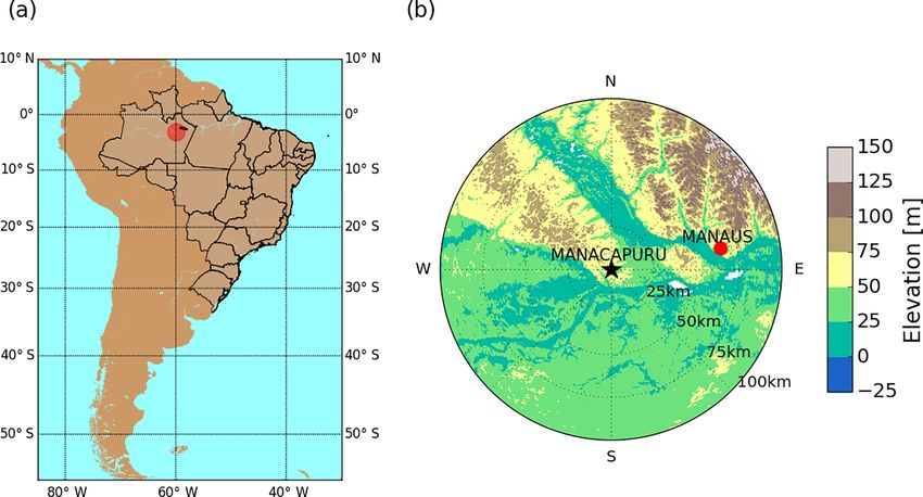
816                                          J.-F. Ribaud et al.: X-band dual-polarization radar-based hydrometeor classification

Table 2. Distance formulas for the weighted, centroid, and Ward
linkage rules. Here, S and T are two clusters joined into a new clus-
ter, whereas V is any another cluster. nS , nT , and nV are the number
of objects contained in the clusters S, T , and V .

    Linkage method    Distance formula for d(S ∪ T , V )
                       d(S,V )+d(T ,V )
    Weighted                  2
                      r
                          nS d(S,V )+nT (T ,V )
    Centroid                     nS +nT         − nS nT d(S,T2 )
                                                   (nS +nT )
                      q
                          (nS +nV )d(S,V )+(nT +nV )d(T ,V )−nV d(S,T )
    Ward                                   nS +nT +nV

       smoothness index is calculated at the end of each iter-
       ation step and individual object by checking the four
                                                                          Figure 3. Evolution of the variance explained for different cluster-
       closest geographical radar gates. In the very same way
                                                                          ing linkage rules. Each linkage method is subdivided in terms of
       as that used in GR15, results are summarized into a con-
                                                                          stratiform (dashed line) and convective (solid line) regions. The or-
       fusion matrix, from which several spatial indexes can              ange vertical span highlights the interval potentially associated with
       be extracted to analyse the individual and global spatial          the optimal number of clusters.
       smoothness of a partition.

     – The merging of two clusters is realized by identify-               (see Table 2 for their respective formulas). Since the clus-
       ing the cluster which presents the lowest spatial sim-             tering method randomly picks observations within the whole
       ilarities among all clusters. Objects belonging to this            wet-season period, a set of numerous runs for each linkage
       spatially poor cluster are then constrained to be redis-           method have been performed to extract, as much as possi-
       tributed through the other existing clusters according to          ble, the most representative behaviour of each one. The gen-
       the linkage method chosen. This final step allows a re-            eral common set-up is composed of a subset of 25 000 obser-
       duction of the total number of clusters by one.                    vations randomly picked through more than 50 precipitation
                                                                          days. The temperature information is based on radiosounding
     – If the iteration process does not reach a single and               observations and is dispatched in a [0;0.5] interval to place
       unique cluster, the iteration loop then restarts at the ini-       twice as much importance on the initial DPOL radar obser-
       tial PPI classification and goes through the evaluation of         vations. The number of clusters reached in the first step of the
       spatial homogeneity.                                               AHC method is set at 50 (far enough from the final partition
                                                                          and not too computationally expensive). Finally, the cluster-
     – Finally, an analysis of the variance explained has been
                                                                          ing method has been conducted separately on stratiform and
       implemented to evaluate the consistency of the clus-
                                                                          convective regions.
       tering classification outputs. This quality metric allows
                                                                             In this respect, Fig. 3 presents the evolution of the vari-
       a definition of the theoretically appropriate number of
                                                                          ance explained (the ratio between the internal and external
       clusters by analysing the ratio between the internal and
                                                                          variance) for the three different linkage rules as a function of
       external variance of each cluster at each step of the iter-
                                                                          the number of clusters considered, together with their asso-
       ation. The main idea here is to find the optimal cluster
                                                                          ciated precipitation regimes (stratiform or convective). Over-
       distribution beyond which considering one more cluster
                                                                          all, the three methods exhibit an “elbow” curvature with an
       is not meaningful.
                                                                          optimal number of clusters ranging from approximately 5 to
                                                                          8 (orange background on Fig. 3). One can see that from 2 to
                                                                          5 clusters, the explained variances sharply increases, mean-
4     Methodology discussions                                             ing that each added cluster within this interval contributes
                                                                          significantly to retrieving the most adequate cluster partition.
4.1     Linkage rule sensitivity                                          From 5 to 8 clusters, the increase starts to slow down, in-
                                                                          dicating that considering a greater number of clusters is not
According to the set-up described in Sect. 3, different link-             meaningful. In this regard, the best compromise seems to be
age rules have been tested through the special wet-season ob-             the weighted and/or Ward linkage method for both stratiform
servation period (February to March) of 2014. To perform                  and convective regions. Indeed, these methods have the high-
this sensitivity test, three different linkage rules have been            est scores, with approximately 99 % reached within the 5–
considered here: (i) weighted, (ii) centroid, and (iii) Ward              8 cluster interval.

Atmos. Meas. Tech., 12, 811–837, 2019                                                          www.atmos-meas-tech.net/12/811/2019/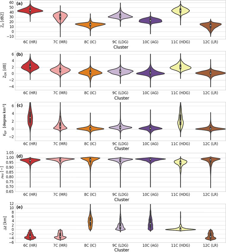
J.-F. Ribaud et al.: X-band dual-polarization radar-based hydrometeor classification 817
Due to the inherent complexity of representing all the cluster 10C). Another discrepancy between the weighted and
potential combinations, manual analysis and selection have Ward linkages concerns the layer around the isotherm at
been performed beforehand to find the optimal number of 0 ◦ C. Although Fig. 5 does not exhibit any bright-band re-
clusters between the stratiform and convective regions. The gion, the Ward linkage rule does exhibit one due to the tem-
results from this partitioning are presented through one strat- perature input (Fig. 5g cluster 12C), whereas the weighted
iform and one convective RHI (Figs. 4 and 5). rule does not. The bright-band region is known to be well
In addition, fuzzy-logic information has been imple- defined for stratiform regimes but quasi-undetectable (if de-
mented to make comparisons with cluster outputs. The tectable at all) for convective areas (Leary and Houze Jr.,
fuzzy-logic scheme is mainly based on the X-band algorithm 1979; Smyth and Illingworth, 1998; Matrosov et al., 2007).
of Dolan and Rutledge (2009), hereafter referred to as DR09, Throughout the present paper, one will thus consider only a
and has been slightly enriched for the wet-snow and melting- bright-band cluster for the stratiform regions, whereas con-
hail hydrometeor types by Besic et al. (2016) through scat- vective areas will be lacking one.
tering simulations and a temperature membership function Overall, Figs. 3, 4, and 5 have shown that the centroid
(Besic et al., 2016, Appendix A). Finally, the adapted fuzzy- linkage method is inappropriate for the present task, whereas
logic allows discrimination between nine hydrometeor types: both weighted and Ward linkage rules are able to retrieve
light rain (LR), rain (RN), melting hail (MH), wet snow a detailed microphysical structure within the sample cloud.
(WS), aggregates (AG), low-density graupel (LDG), high- Based on the present description and our personal analysis
density graupel (HDG), vertically aligned ice (VI), and ice over the whole dataset, we chose to keep working with the
crystals (IC). weighted linkage rule throughout the remainder of the paper.
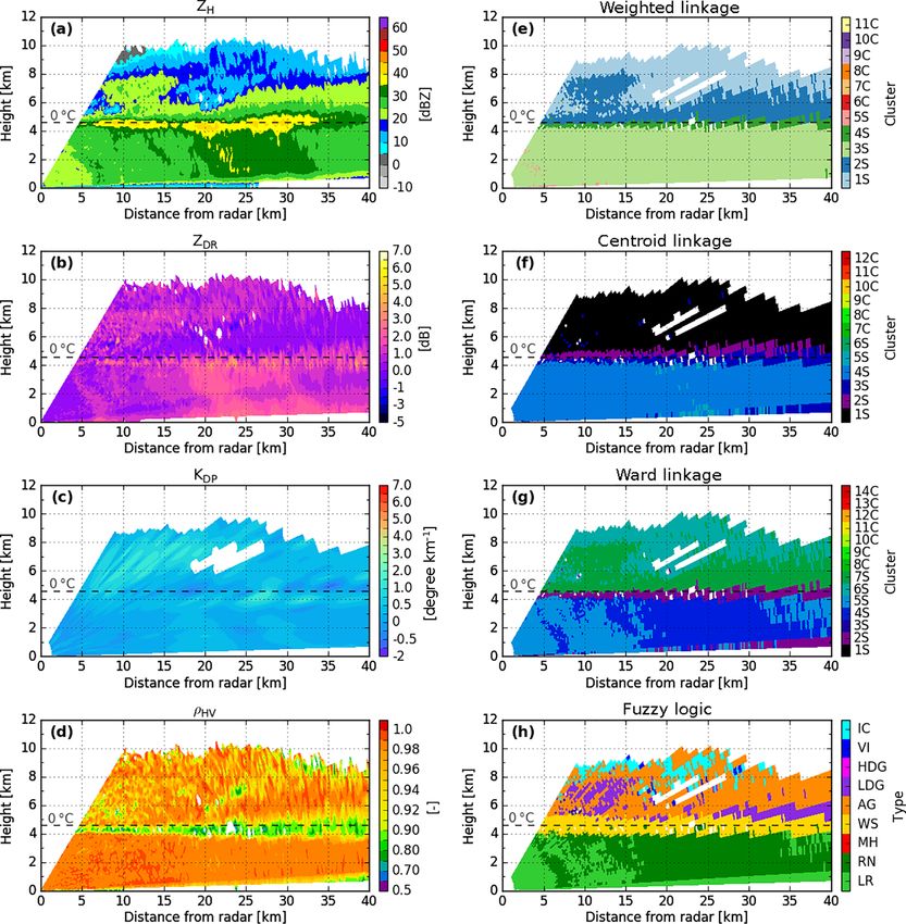
Figure 4 shows a stratiform system exhibiting a well-
defined bright-band signature from polarimetric observations
4.2 Potential improvement around isotherm 0 ◦ C
that occurred on the shores of the Amazon River on 21 Febru-
ary 2014. Overall, the centroid linkage method does not re-
produce the event well, and the final representation is mi- High amounts of liquid water a few kilometres above the
crophysically poor (Fig. 4f). Indeed, this linkage rule simply isotherm at 0 ◦ C are not rare within the core of convective
divides the cloud into three homogeneous regions (T > 0 ◦ C, tropical cells. Sometimes, super-cooled liquid drops can be
T ∼ 0 ◦ C, and T < 0 ◦ C). Additionally, the centroid linkage maintained and even moved upward within the melting layer,
fails to identify a clear bright-band region (Fig. 4f, clus- thus occasionally giving distinctive column-shaped polari-
ters 2S and 3S). On the other hand, the weighted and Ward metric signatures for ZDR /KDP (e.g. Kumjian and Ryzhkov,
linkage methods are very close to the fuzzy-logic output de- 2008). A simple liquid–solid delineation based only on the
scriptions (Fig. 4e, g, h). They both exhibit two kinds of rain, temperature profile is therefore unsuitable.
and a bright-band region sits below what appears to be an Figure 6 presents an adaptive solution for tackling this is-
aggregate–ice crystals mixture. The main discrepancy here sue based on the clustering outputs of the weighted linkage
concerns the representation of the rain structure. The Ward rule. The solution proposed here relies on a posteriori anal-
linkage rule retrieves two more distinct liquid species (as ysis of the clustering outputs associated with the convective
does fuzzy logic), whereas the weighted linkage method ex- regions. First, one proceeds to identify the convective core
hibits a smoother rainy region. under the isotherm at 0 ◦ C (here, cluster 6C). Then, all radar
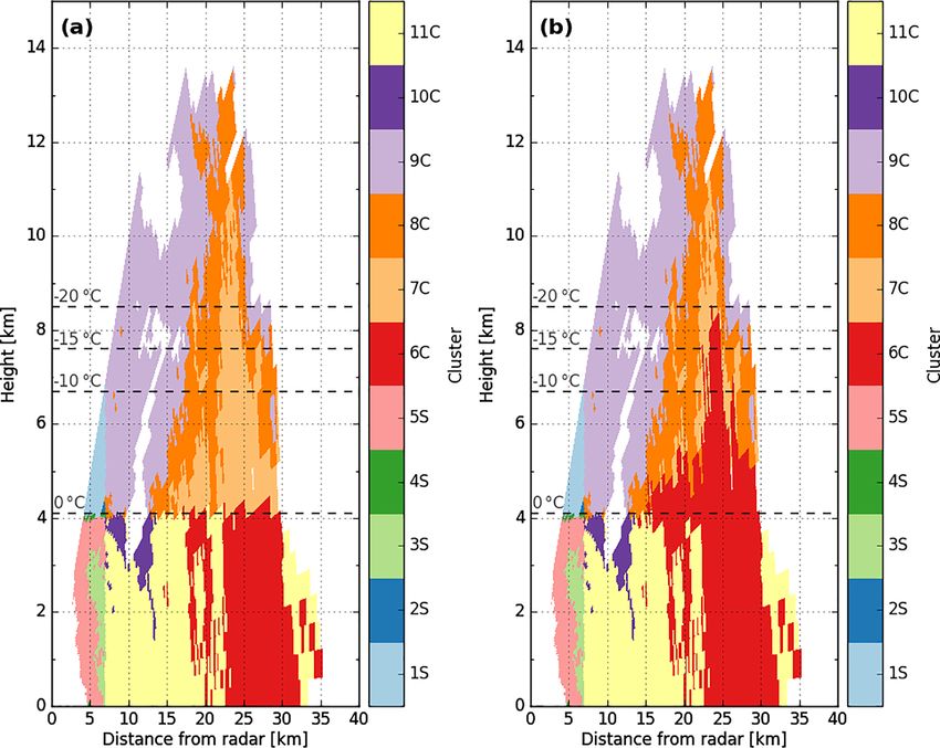
Figure 5 presents a decaying convective cell that occurred observations within the solid region are assigned by calcu-
on 2 February 2014 at 13:57 UTC (0–7 km from the radar: lating their distance from the 6C cluster centroid without ap-
stratiform region, 7–40 km from the radar: convective re- plying any temperature constraint (objects are thus defined
gion). As is the case for the stratiform RHI in Fig. 4, the only by the first four radar components). If the distance is
centroid linkage rule fails to retrieve a detailed microphysi- smaller than D < 0.25 and there is no discontinuity through-
cal structure and only presents very homogeneous liquid and out the liquid–solid delineation, then the solid identification
solid regions. Once again, both the weighted and the Ward is switched to liquid (cluster 6C). Note that the distance D
linkage rules stand out and display a more realistic hydrom- has been empirically chosen for the present radar observa-
eteor description of the convective cloud in comparison to tions and could consequently be adjusted by exploring more
the DPOL radar observations and the fuzzy-logic outputs convective days. Overall, with this simple hypothesis, one
(Fig. 5a–e, g, h). Although they both present three clusters can see the potential of a such method (Fig. 6b). The liquid
for T > 0 ◦ C, the weighted linkage rule puts more emphasis cluster can thus reach 8 km in the core of the convection at
on the convective region located ∼ 20–30 km from the radar 25 km from the radar, which matches well with the convec-
than does the Ward linkage (Fig. 5e, cluster 6C vs. Fig. 5g, tive tower (> 35 dBZ) visible in Fig. 5a. Around this con-
cluster 11C). The representation of the solid region (T < vective core, the enhancement allows raindrops to be raised
0 ◦ C) is almost the same, except for in the aggregate region by about 1 km upward in the 0 ◦ C isotherm, restraining clus-
(Fig. 5h), which seems to be smaller for the weighted linkage ter 6C at ∼ 5 km. In comparison to a simple binary delin-
rule (Fig. 5e cluster 8C) than for the Ward method (Fig. 5g eation such as that used for the fuzzy-logic outputs (Fig. 6a),
www.atmos-meas-tech.net/12/811/2019/ Atmos. Meas. Tech., 12, 811–837, 2019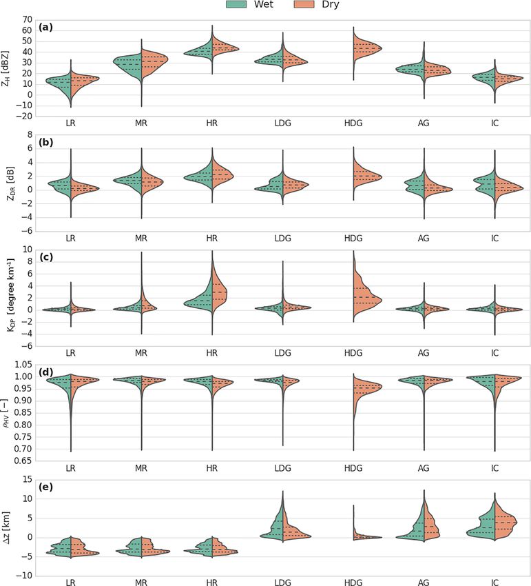
818                                    J.-F. Ribaud et al.: X-band dual-polarization radar-based hydrometeor classification

Figure 4. X-band DPOL radar observables and the corresponding retrieved hydrometeor classification outputs at 12:07 UTC on 21 Febru-
ary 2014, along the azimuth 290◦ . DPOL radar observables are shown in (a) ZH , (b) ZDR , (c) KDP , and (d) pHV . Comparisons of retrieved
hydrometeors for clustering outputs based on (e) weighted, (f) centroid, and (g) Ward linkage rules and (h) fuzzy-logic scheme outputs. In
(e)–(g), each number corresponds to a different cluster. S stands for stratiform regimes, whereas C is for convective regimes.

the focus on radar observables in a second phase is then               5   Wet- and dry-season-dominant hydrometeor
promising.                                                                 classifications

                                                                       This section aims to interpret and label each cluster retrieved
                                                                       through both the wet and dry seasons over the Manaus re-
                                                                       gion by using the AHC method set-up described in Sect. 3.
                                                                       As the use of classification allowing liquid water above the

Atmos. Meas. Tech., 12, 811–837, 2019                                                       www.atmos-meas-tech.net/12/811/2019/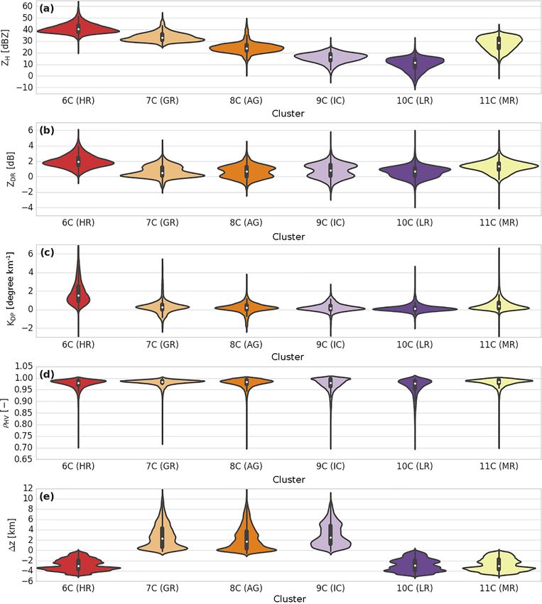
J.-F. Ribaud et al.: X-band dual-polarization radar-based hydrometeor classification                                          819

Figure 5. Same as Fig. 4, but for 13:57 UTC on 13 February 2014, along the azimuth 200◦ .

melting layer of convective towers needs further validation, a        ble between the stratiform (convective) clustering outputs
standard classification is used to classify and analyse the wet       and the nine microphysical species retrieved by the DR09
and dry hydrometeors using the temperature parameter.                 adapted fuzzy-logic algorithm is shown in Table 3 (Table 4).
                                                                      The complete wet-season cluster centroids are given in Ap-
5.1   Wet-season clustering outputs                                   pendix Table A1.

The distributions of ZH , ZDR , KDP , ρHV , and 1z for each           5.1.1   Stratiform region
cluster from the stratiform and convective clouds of the wet
season together with their probability densities are presented        Cluster 1S is only defined for negative temperatures and is
in the violin plot in Figs. 7 and 8. The contingency ta-              associated with high ρHV and low ZH , ZDR , and KDP val-

www.atmos-meas-tech.net/12/811/2019/                                                        Atmos. Meas. Tech., 12, 811–837, 2019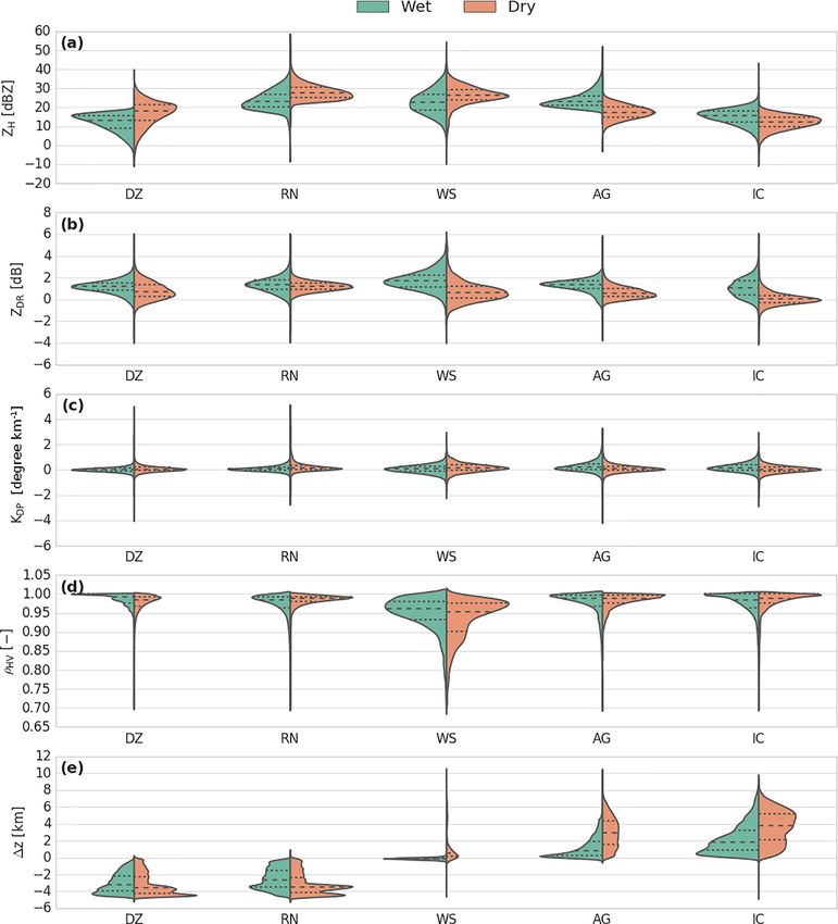
820                                    J.-F. Ribaud et al.: X-band dual-polarization radar-based hydrometeor classification

Figure 6. Clustering hydrometeor classification retrieved from the X-band radar at 12:07 UTC on 21 February 2014, along the azimuth 290◦ .
(a) With temperature constraint, (b) without temperature constraint.

Table 3. Confusion matrix comparing the clustering outputs from the stratiform region of the wet season and hydrometeor species retrieved
from the adapted fuzzy logic.

                TYPE           DZ         RN       MH          WS         AG        LDG       HDG          VI        CR
                1S        38.64 %     0.01 %    0.00 %     10.34 %    32.91 %     1.31 %    0.00 %     4.47 %    12.34 %
                2S         0.02 %     0.21 %    0.00 %     43.51 %    42.66 %    11.91 %    0.00 %     0.02 %     1.67 %
                3S        64.36 %    27.55 %    0.21 %      7.88 %     0.00 %     0.00 %    0.00 %     0.00 %     0.00 %
                4S         5.75 %     7.27 %    0.02 %     86.02 %     0.53 %     0.11 %    0.00 %     0.03 %     0.27 %
                5S        98.04 %     0.00 %    0.27 %      1.68 %     0.00 %     0.00 %    0.00 %     0.00 %     0.00 %

ues (Figs. 4e and 7). One can see from contingency Table 3             of fuzzy logic (Table 3). Figure 4e allows discrimination be-
that the cluster 1S repartition is mostly associated with aggre-       tween these categories, and one can consider that here clus-
gates (∼ 33 %) and ice crystals (∼ 12 %) for high altitudes.           ter 2S is associated with aggregates. Once again, its polari-
Although the horizontal and differential reflectivity values           metric signatures are slightly higher than the DR09 T-matrix
are slightly higher than those for the DR09 T-matrix micro-            values or even the GR15 aggregate clustering output. One ex-
physical outputs and polarimetric characteristics retrieved by         plication behind these distributions being slightly shifted to
GR15, one can make the assumption that the cluster 1S be-              higher values can be the relative humidity, which is higher in
haviour stands for ice crystals. On the other hand, cluster 2S         the tropics than at higher latitudes. The growth of ice crys-
is closer to the DR09 T-matrix aggregates of microphysical             tals/aggregates by vapour diffusion within this cloud region
features. This cluster is characterized by a mean horizon-             (Houze, 1997) may lead to bigger solid particles (higher ZH
tal (differential) reflectivity of ∼ 27 dBZ (∼ 1.3 dB), a low          and ZDR values).
specific differential phase (∼ 0.27 ◦ km−1 ), and a high coef-            The bright-band region is well represented here by clus-
ficient of correlation (0.97). Overall, the polarimetric signa-        ter 4S. Indeed, its global distribution spreads only at the al-
tures of cluster 2S are mostly divided into the associated wet         titude of the isotherm at 0 ◦ C and exhibits high ZH and ZDR
and dry snow (aggregates) from the microphysical categories            values, as well as low KDP and ρHV values. Finally, clus-

Atmos. Meas. Tech., 12, 811–837, 2019                                                       www.atmos-meas-tech.net/12/811/2019/
J.-F. Ribaud et al.: X-band dual-polarization radar-based hydrometeor classification 821
Table 4. Same as Table 3, but for the convective region of the wet season.
TYPE DZ RN MH WS AG LDG HDG VI CR
6C 77.00 % 21.70 % 0.99 % 0.31 % 0.00 % 0.00 % 0.00 % 0.00 % 0.00 %
7C 0.00 % 0.16 % 0.00 % 21.69 % 7.70 % 69.01 % 1.44 % 0.00 % 0.00 %
8C 0.78 % 2.70 % 0.02 % 27.24 % 44.51 % 23.71 % 0.00 % 0.27 % 0.77 %
9C 0.10 % 0.00 % 0.00 % 9.86 % 55.90 % 5.83 % 0.00 % 9.15 % 19.16 %
10C 96.47 % 0.14 % 1.46 % 1.92 % 0.00 % 0.00 % 0.00 % 0.00 % 0.00 %
11C 31.42 % 62.98 % 1.24 % 4.36 % 0.00 % 0.00 % 0.00 % 0.00 % 0.00 %
Figure 7. Violin plot of cluster outputs retrieved for the stratiform regime of the wet season (DZ is drizzle, RN is rain, WS is wet snow, AG
is aggregates, and IC is ice crystals). The thick black bar in the centre represents the interquartile range, and the thin black line extended from
it represents the 95 % confidence intervals, while the white dot is the median.
www.atmos-meas-tech.net/12/811/2019/ Atmos. Meas. Tech., 12, 811–837, 2019822 J.-F. Ribaud et al.: X-band dual-polarization radar-based hydrometeor classification
Figure 8. Same as Fig. 7, but for the convective regime of the wet season (LR is light rain, MR is moderate rain, HR is heavy rain, GR is
graupel, AG is aggregates, and IC is ice crystals).
ters 3S and 5S present rain characteristics, since more than 5.1.2 Convective region
90 % of these clusters are in agreement with the drizzle and
rain fuzzy-logic types from DR09. Although the two clus-
ters have the same behaviour, cluster 3S is characterized by Overall, one can see from Figs. 5 and 8 that the convective
polarimetric signatures higher than those in cluster 5S, ex- regions of the wet season are composed of three types of hy-
cept for the coefficient of correlation (0.97 vs. 0.99). In this drometeors for both positive (clusters 6C, 10C, and11C) and
regard, one can consider that cluster 3S represents the rain negative temperatures (clusters 7C, 8C, and 9C).
microphysical species, whereas cluster 5S is related to driz- Hail precipitation in the Amazonas region is rare, and as
zle characteristics. expected, no clusters represent melting hail characteristics,
as in Ryzhkov et al. (2013) or Besic et al. (2016) (Table 4).
Therefore, clusters 6C, 10C, and 11C can be associated with
Atmos. Meas. Tech., 12, 811–837, 2019 www.atmos-meas-tech.net/12/811/2019/J.-F. Ribaud et al.: X-band dual-polarization radar-based hydrometeor classification 823
three distinct rainfall precipitation regimes. In this regard, ative temperatures, clusters 3S–5S show patterns close to the
cluster 10C presents the same light-rain characteristics as fuzzy-logic outputs.
both DR09 and GR15. The cluster is characterized by ZH The violin plots in Fig. 10 and contingency Table 5 al-
(ZDR ) values approximately 13 dBZ (0.68 dB), and a KDP low discrimination and labelling of these clusters. For DR09
(0.14 ◦ km−1 ) that is in high agreement with the drizzle hy- classification, clusters 1S and 2S exhibit rainfall signatures.
drometeor type from the adapted fuzzy logic (∼ 97 %, Ta- Cluster 2S is in agreement with the fuzzy-logic drizzle cate-
ble 4). According to this description, one can attribute clus- gory (∼ 92 %), whereas cluster 1S is divided into the drizzle
ter 11C to the light-rain precipitation type. The two remain- (∼ 76 %) and rain (∼ 22 %) microphysical species. Between
ing liquid clusters are associated with moderate and heavy these two clusters, one can observe that cluster 1S contains
rainfall types with almost the same polarimetric signatures the highest ZH , ZDR and KDP values, and one can conse-
as those given in GR15. Indeed, cluster 6C presents higher quently label it as a rainfall type. Cluster 2S is, however, as-
ZH (44 vs. 31 dBZ), ZDR (2.1 vs. 1.4 dB), and KDP (1.9 sociated with the drizzle/light-rain category according to the
vs. 0.8 ◦ km−1 ) mean values than those for cluster 11C. In polarimetric radar signatures (GR15).
this regard, one can link cluster 6C to heavy rainfall and clus- The liquid–solid delineation is represented here by clus-
ter 11C to moderate rainfall. ter 4S. It presents a low ρHV (∼ 0.93) and a large ZH dis-
Concerning negative temperatures, cluster 9C stands out tribution around ∼ 30 dBZ and is almost only defined for al-
by being spread at the highest altitudes (Fig. 8e). This cluster titudes close to the 0 ◦ C isotherm. In addition, contingency
is defined by low ZH , ZDR , and KDP values together with a Table 5 matches well with this hydrometeor association.
moderate ρHV (∼ 0.97). One can note that cluster 9C is close For the negative temperatures, the clustering outputs ex-
to the ice crystals and small aggregates retrieved by GR15 hibit two clusters, 3S–5S. The first is located within the
and is also the only cluster related to the T-matrix ice crystals edge region of the cloud, whereas cluster 5S is distributed at
species from DR09 (Table 4). Within the decaying convective lower altitudes and is closer to particles of greater densities
cell presented in Fig. 5, one can observe that cluster 7C is (Fig. 10). Cluster 5S is in ∼ 70 % agreement with the aggre-
associated with the low-density graupel characteristics pro- gate fuzzy-logic outputs (Table 5), and its polarimetric sig-
posed by DR09 and exhibits ZH (ZDR ) values approximately natures are close to those of GR15 and T-matrix simulations
36 dBZ (0.8 dB). In addition, cluster 7C is mainly classified from DR09. One can then define cluster 5S as the aggregate
(∼ 69 %) as low-density graupel (Table 4). Finally, the last microphysical species. Finally, ice crystals and small aggre-
cluster, 8C, is surrounded by ice crystals and presents polari- gates are represented through cluster 3S, which is defined by
metric signatures lower than those for cluster 7C. Although low ZH , ZDR , and KDP values and a high ρHV .
it is defined by higher values than those given by DR09 and
GR15, one can associate cluster 8C with the aggregate mi- 5.2.2 Convective region
crophysical species. Indeed, contingency Table 4 shows that
45 % of the cluster 8C points are in agreement with this hy- Figure 11 shows an RHI of a convective system that occurred
drometeor type. in the late afternoon on 6 October 2014 in the region of Man-
aus. Overall, this RHI shows a convective cell (at 24–50 km
5.2 Dry-season clustering outputs from the radar) together with its relative stratiform region (0–
23 km). Note that the abrupt transition from the convective
and stratiform classification areas (Figs. 5, 6, 11) is inherent
As for the previous section, the clustering outputs retrieved
to the Steiner et al. (1995) algorithm. In terms of microphys-
by the AHC method and the weighted linkage rule are iden-
ical distribution, there should be some consistency between
tified and associated with their corresponding microphysical
the two cloud types. The implementation of continuity anal-
species through the dry tropical season. The corresponding
ysis may prevent the latter artefacts. The convective cell is
cluster centroids are detailed in Appendix Table A2.
characterized by ZH values up to 25 dBZ at 14 km, and the
cloud top exceeds 16 km. According to the fuzzy-logic out-
5.2.1 Stratiform region puts (Fig. 11f), the cell mostly exhibits rainfall precipitation
for positive temperatures. The corresponding cluster outputs
Figure 9 shows the clustering classification outputs extracted retrieve the same signatures, dividing the rain pattern into
from an RHI presenting a melting layer region within a strat- three different clusters: 6C, 7C, and 12C. Once again, the
iform event that occurred on 8 September 2014 in the re- fuzzy logic collocates a bright band around the isotherm at
gion of Manaus. Overall, the clustering outputs are close to 0 ◦ C, whereas neither polarimetric signatures nor clustering
the hydrometeor distribution retrieved by the adapted DR09 outputs exhibit a bright band. For negative temperatures, the
fuzzy logic. Clusters 1S–2S retrieved for positive tempera- AHC method retrieves four clusters (8C, 9C, 10C, and 11C),
tures appear well located in terms of polarimetric signatures the same as the fuzzy-logic outputs.
and fuzzy-logic outputs. One can see that the melting layer The violin plots in Fig. 12 and contingency Table 6 allow
region is clearly characterized by cluster 4S, whereas for neg- discrimination and labelling of these clusters. For the con-
www.atmos-meas-tech.net/12/811/2019/ Atmos. Meas. Tech., 12, 811–837, 2019824 J.-F. Ribaud et al.: X-band dual-polarization radar-based hydrometeor classification Figure 9. X-band DPOL radar observables and the corresponding retrieved hydrometeor classification outputs at 21:26 UTC on 8 Septem- ber 2014, along the azimuth 200◦ . DPOL radar observables are shown in (a) ZH , (b) ZDR , (c) KDP , and (d) pHV . Comparisons of retrieved hydrometeors for clustering outputs based on (e) weighted linkage rules and (f) the fuzzy-logic scheme. In (e)–(f), each number corresponds to a different cluster. S stands for the stratiform region, whereas C is for the convective region. vective regions observed during the wet season, hail precipi- lower values than cluster 6C (Fig. 12). In addition, one can tation is rare in the Amazonas. Contingency Table 6 is also in see from contingency Table 6 that all three are in very high agreement with this description, since none of the clustering agreement with the drizzle and rain microphysical species. outputs exceed 3 %. Therefore, one can attribute clusters 6C, Based on the aforementioned description together with the 7C, and 12C to three different rainfall precipitation regimes, Fig. 11 analysis, one can attribute cluster 12C to light rain- ranking the cluster positions as follows: 12C presents weaker fall, cluster 7C to moderate rainfall and, finally, cluster 6C to ZH , ZDR , and KDP values than cluster 7C, which presents the heavy-rainfall type. Atmos. Meas. Tech., 12, 811–837, 2019 www.atmos-meas-tech.net/12/811/2019/
J.-F. Ribaud et al.: X-band dual-polarization radar-based hydrometeor classification                                                   825

Figure 10. Same as Fig. 7, but for the stratiform regime of the dry season (DZ is drizzle, RN is rain, WS is wet snow, AG is aggregates, and
IC is ice crystals).

Table 5. Same as Table 3, but for the stratiform region of the dry season.

                TYPE           DZ          RN       MH          WS           AG      LDG       HDG           VI         CR
                1S        76.30 %     22.17 %    0.10 %      1.43 %      0.00 %    0.00 %    0.00 %     0.00 %      0.00 %
                2S        92.32 %      4.36 %    0.65 %      2.63 %      0.02 %    0.00 %    0.00 %     0.01 %      0.00 %
                3S         0.25 %      0.00 %    0.00 %      2.65 %     41.61 %    2.19 %    0.00 %    21.18 %     32.12 %
                4S         0.97 %      1.30 %    0.00 %     49.30 %     18.46 %   26.83 %    0.23 %     0.44 %      2.48 %
                5S         0.30 %      0.03 %    0.00 %      8.28 %     68.48 %    3.99 %    0.00 %     5.29 %     13.62 %

www.atmos-meas-tech.net/12/811/2019/                                                          Atmos. Meas. Tech., 12, 811–837, 2019
826 J.-F. Ribaud et al.: X-band dual-polarization radar-based hydrometeor classification Figure 11. Same as Fig. 9, but for an RHI at 18:16 UTC on 6 October 2014, along the azimuth 200◦ . Concerning all clusters spreading at negative tempera- hail, as suggested by Straka et al. (2000) and Kumjian and tures, cluster 11C matches well with the high-density grau- Ryzhkov (2008). This cloud region is surrounded by low- pel category defined by DR09 such as “graupel growing in density graupel, characterized by cluster 9C (Figs. 11–12). regions of large supercooled water contents, melting grau- This hydrometeor type shows 60 % agreement with this mi- pel, and freezing of supercooled rain”. Based on contingency crophysical type within contingency Table 6 and is close to Table 6, this cluster is mainly associated with wet snow and the DR09 T-matrix outputs. Cluster 10C shares more than slightly with the low-density graupel microphysical specie. 50 % with the aggregate type and 30 % with the low-density Nevertheless, one can see that the ρHV distribution is pretty graupel type, whereas cluster 8C is associated in general with low (∼ 0.94) and could also be the signature of wet graupel ice crystals and aggregate types (Table 6). With Figs. 11–12 (due to melting or wet growth) or a mixture of graupel and and the aforementioned description, one can analyse clus- Atmos. Meas. Tech., 12, 811–837, 2019 www.atmos-meas-tech.net/12/811/2019/
J.-F. Ribaud et al.: X-band dual-polarization radar-based hydrometeor classification                                                  827

Figure 12. Same as Fig. 7, but for the convective regime of the dry season (LR is light rain, MR is moderate rain, HR is heavy rain, LDG is
low-density graupel, HDG is high-density graupel, AG is aggregates, and IC is ice crystals).

Table 6. Same as Table 3, but for the stratiform region of the dry season.

                TYPE           DZ          RN       MH          WS           AG     LDG       HDG           VI         CR
                6C        73.71 %     23.34 %    2.60 %      0.34 %      0.00 %    0.00 %   0.00 %      0.00 %     0.00 %
                7C        21.61 %     73.56 %    1.00 %      3.83 %      0.01 %    0.00 %   0.00 %      0.00 %     0.00 %
                8C         0.07 %      0.01 %    0.00 %      5.62 %     51.01 %    2.70 %   0.00 %     12.72 %    27.87 %
                9C         0.16 %      2.32 %    0.00 %     27.80 %      7.41 %   60.40 %   1.86 %      0.00 %     0.04 %
                10C        0.79 %      0.17 %    0.00 %     13.48 %     51.19 %   30.91 %   0.00 %      0.83 %     2.63 %
                11C        0.00 %     15.29 %    0.51 %     64.19 %      0.19 %    11.4 %   7.72 %      0.00 %     0.00 %
                12C       97.19 %      0.00 %    0.41 %      2.34 %      0.06 %    0.00 %   0.00 %      0.01 %     0.00 %

www.atmos-meas-tech.net/12/811/2019/                                                         Atmos. Meas. Tech., 12, 811–837, 2019
828 J.-F. Ribaud et al.: X-band dual-polarization radar-based hydrometeor classification
ter 9C as low-density graupel, cluster 10C as aggregates, and, 6.2 Wet–dry season differences
finally, cluster 8C as ice crystals.
The investigation of some Amazonian wet–dry season dif-
ferences has already been explored by a few studies. For
6 Discussion instance, Machado et al. (2018) noted that, during both
the GoAmazon2014/5 and ACRIDICON-CHUVA field cam-
6.1 Impact of the clustering method and location paigns, the wet-season overall mean cumulative rain was 4
times as much as that during the dry season. However, though
The present results allow us to make a brief comparison characterized by a low amount of total rainfall, the dry season
of the classical supervised fuzzy-logic technique commonly presents the higher rainfall rate (Dolan et al., 2013; Machado
used in the literature and the unsupervised AHC method. et al., 2018). According to Machado et al. (2018), these dis-
In opposition to the rigid structure of a fuzzy-logic algo- crepancies can partly be explained by the fact that the dry
rithm, the flexibility of the clustering approach allows better season presents higher convective available potential energy
identification of the bright-band region. Indeed, the liquid– (CAPE) and lower cloud cover than the wet season. Another
solid delineation around the 0 ◦ C isotherm is better captured study conducted by Giangrande et al. (2017) also examined
and distinguished by the AHC method, which preferentially the wet–dry season differences through convective clouds.
follows the polarimetric signatures instead of the stratified The authors showed that warm clouds exhibit larger cloud
temperature region. Additionally, one can see the ability of droplets and that the stratiform region during the wet season
the AHC method to fully exploit the high sensitivity of the is much more developed than during the dry season (due to
X-band radar frequency to distinguish between three differ- surrounding monsoon ambient characteristics).
ent (light, moderate, and heavy) rainfall regimes such as in All these differences are expected to contribute to the wet–
GR15. This enhancement allows, for instance, for more em- dry season differences. Here, one can address for the first
phasis on severe convective precipitation cells and may open time these discrepancies through the dominant microphysical
new perspectives for nowcasting issues. patterns in terms of stratiform and convection precipitation
Note that the present clustering method has been distinctly regimes associated with the Central Amazonas (Manaus re-
subdivided into stratiform and convective regions. Although gion). Based on this new hydrometeor classification adapted
they are characterized by different thermodynamic structures to the tropical region, this section explores the differences
(Houze, 1997), the stratiform and convective regions may be among the clouds related to these two seasons.
related in terms of microphysical distributions, such as ice
particles which might be ejected from the top of an active 6.2.1 Stratiform region
convective cell into the upper part of the stratiform region.
This microphysical continuity could be further considered ei- Figure 13 presents a comparison of pairs of stratiform hy-
ther by merging stratiform and convective hydrometeor types drometeor types between the wet and dry seasons. For pos-
that present close DPOL characteristics (Figs. 7, 8, 10, and itive temperatures, both the drizzle and rain microphysical
12) or by implementing an a posteriori continuity analysis. species present higher ZH and lower ZDR values during the
The location of the present study also offers the possibil- dry season than during the wet season. These polarimetric
ity of discussing midlatitude and tropical microphysical dif- signatures might be attributed to the evaporation and colli-
ferences. As described in Sect. 5, the dominant tropical hy- sional processes that tend to reduce the particle diameters
drometeor classification overlaps with some midlatitude mi- (Kumjian and Ryzhkov, 2010; Penide et al., 2013). The sep-
crophysical species definitions. For instance, one can see that aration between the drizzle/light rain and the rain microphys-
both the aggregate and ice crystal microphysical species are ical species is defined for a rainfall rate of approximately
skewed to higher horizontal (differential) reflectivity, regard- 2.5 mm h−1 (American Meteorological Society, 2018). The
less of the season and region (stratiform/convective) consid- classical Marshall–Palmer Z–R relationship allows an esti-
ered. These discrepancies might be attributed either to an in- mation of the rainfall rate for stratiform precipitation. In this
accurate attenuation correction or inherent tropical charac- regard, the wet-rain microphysical species is characterized,
teristics involved within microphysical ice growth. Although on average, by a rainfall rate of 1.84 mm h−1 , whereas the
we considered a limited radar coverage, regions with high rate is up to 3 mm h−1 during the dry season. The general
SNR values, as well as precipitation-only events having a wet-rain microphysical species distribution thus still contains
dry radome, the ZPHI method may still lead to overcorrec- drizzle/light-rain observations, which might be due to the dif-
tion, especially on ZDR in strong convective cases when the ferent cloud cover patterns associated with stratiform echoes
Mie scattering may dominate the precipitation regions. An- during the two seasons. As noted by Machado et al. (2018),
other explanation of these discrepancies may rely on tropical stratiform cloud cover related to the rainy season is more as-
atmospheric characteristics that present higher tropospheric sociated with a monsoon cloud regime than during the re-
humidity profiles together with higher incident solar radia- maining season. While the dry season stratiform regime is
tion, playing an important role in comparison to midlatitudes. directly the result of the rain convective cells, the wet strati-
Atmos. Meas. Tech., 12, 811–837, 2019 www.atmos-meas-tech.net/12/811/2019/You can also read