Continental-Scale Land Cover Mapping at 10 m Resolution over Europe (ELC10)

Page created by Chad Conner
 
CONTINUE READING
Continental-Scale Land Cover Mapping at 10 m Resolution over Europe (ELC10)
remote sensing
Article
Continental-Scale Land Cover Mapping at 10 m Resolution over
Europe (ELC10)
Zander S. Venter *             and Markus A. K. Sydenham

                                          Norwegian Institute for Nature Research—NINA, Sognsveien 68, 0855 Oslo, Norway;
                                          markus.sydenham@nina.no
                                          * Correspondence: zander.venter@nina.no

                                          Abstract: Land cover maps are important tools for quantifying the human footprint on the environ-
                                          ment and facilitate reporting and accounting to international agreements addressing the Sustainable
                                          Development Goals. Widely used European land cover maps such as CORINE (Coordination of
                                          Information on the Environment) are produced at medium spatial resolutions (100 m) and rely on
                                          diverse data with complex workflows requiring significant institutional capacity. We present a 10 m
                                          resolution land cover map (ELC10) of Europe based on a satellite-driven machine learning workflow
                                          that is annually updatable. A random forest classification model was trained on 70K ground-truth
                                          points from the LUCAS (Land Use/Cover Area Frame Survey) dataset. Within the Google Earth
                                          Engine cloud computing environment, the ELC10 map can be generated from approx. 700 TB of
                                          Sentinel imagery within approx. 4 days from a single research user account. The map achieved an
                                          overall accuracy of 90% across eight land cover classes and could account for statistical unit land
                                          cover proportions within 3.9% (R2 = 0.83) of the actual value. These accuracies are higher than that
                                of CORINE (100 m) and other 10 m land cover maps including S2GLC and FROM-GLC10. Spectro-
         
                                          temporal metrics that capture the phenology of land cover classes were most important in producing
Citation: Venter, Z.S.; Sydenham,
                                          high mapping accuracies. We found that the atmospheric correction of Sentinel-2 and the speckle
M.A.K. Continental-Scale Land Cover
                                          filtering of Sentinel-1 imagery had a minimal effect on enhancing the classification accuracy (
Continental-Scale Land Cover Mapping at 10 m Resolution over Europe (ELC10)
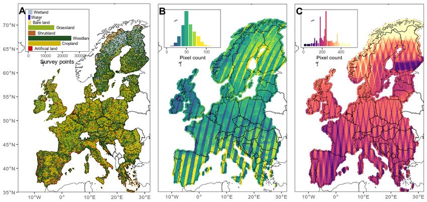
Remote Sens. 2021, 13, 2301                                                                                          2 of 22

                              for meeting SDG 2 of zero hunger and SDG 15 to monitor efforts to reduce natural habitat
                              loss (e.g., deforestation alerts). Ecosystem service models and accounts also rely on land
                              cover data as input [5] and land cover maps are thereby important for the valuation and
                              conservation of important ecosystems. In light of global climate change and a rapidly
                              developing world, an increasing number of applications, such as precision agriculture,
                              wildlife habitat management, urban planning, and renewable energy installations, require
                              higher resolution and frequently updated land cover maps.
                                    The advent of cloud computing platforms like the Google Earth Engine [6] has led
                              to significant advances in the ability to map land surface changes over time [7,8]. This is
                              both due to the enhanced computing power and the availability of dense time series data
                              from medium to high resolution sensors like Sentinel-2 [9]. The transition to time series
                              imagery allows one to capture the seasonal and phenological components of land cover
                              classes that would otherwise be missed with single time-slice imagery. The application
                              of such spectro-temporal metrics to mapping forest [10] and other land cover types [11]
                              has shown increased classification accuracies. In addition, the ability to adopt machine
                              learning algorithms in cloud computing environments has further enhanced the precision
                              of land cover mapping [4].
                                    The CORINE (Coordination of Information on the Environment) land cover map of
                              Europe [12] is perhaps the most widely used land cover product for area statistics and
                              research [13]. The CORINE map currently requires significant institutional capacity and
                              coordination from the European member states, the Eionet network, and the European
                              Environmental Agency. For instance, the 2012 product involved 39 countries, a diver-
                              sity of country-specific topographic and remote sensing datasets and took two years to
                              complete. To ease the manual workload, the wealth of data from the Copernicus Sen-
                              tinel sensors has been somewhat integrated into the CORINE mapping workflow and has
                              also led to the development of Copernicus Land cover services high spatial resolution
                              maps (https://land.copernicus.eu/pan-european/high-resolution-layers, accessed on 15
                              May 2021). Recently, Sentinel-2 data have been used to create a 10 m pan-European
                              land cover/use map (S2GLC) for cairca 2017 (http://s2glc.cbk.waw.pl/, accessed on
                              15 May 2021) [14]. This is a meaningful advancement on previous pan-European map-
                              ping efforts, however, the methodology behind S2GLC involves a land cover reference
                              dataset and some post-processing steps that are not open source or easily reproducible.
                              Pflugmacher et al. [15] recently developed an independent, research-driven approach to
                              pan-European land cover mapping with Landsat data at 30 m for cairca 2015. This compares
                              favourably with the CORINE map, is reproducible and does not require harmonising and
                              collating country-specific datasets from different European member states. Nevertheless,
                              there remains potential for a similar open source approach that leverages both Sentinel-2
                              optical and Sentinel-1 radar sensor data to map land cover at 10 m resolution [16].
                                    Land cover maps made with open data policies and open science principles can have
                              transfer value to other areas of the globe [17], particularly when pre- and post-processing
                              decisions are made transparent. Like the European maps mentioned above, the studies doc-
                              umenting continental land cover classifications at 30- or 10-m resolution for Africa [18,19],
                              North America [20] and Australia [21] have not communicated methodological lessons
                              or published source codes. The same is true for global land cover products such as the
                              Landsat-based GLOBLAND30 [22] or Sentinel-based FROM-GLC10 [23]. This makes it
                              difficult to draw generalizable conclusions that the benefit of remote sensing and the
                              land cover mapping community at large. Specifically, it is not clear how satellite and
                              reference data pre-processing decisions affect the accuracy of land cover classifications
                              at this scale. Such decisions may concern the atmospheric correction of optical imagery
                              (Sentinel-2), the speckle filtering of radar imagery (Sentinel-1), or the fusion of optical
                              and radar data within one classification model. When trying to classify land cover over
                              very broad environmental gradients where spectral signatures vary substantially within
                              a given land cover class, one may also decide to include auxiliary variables to increase
                              model accuracy [15]. Such decisions have trade-offs between computational efficiency and
Continental-Scale Land Cover Mapping at 10 m Resolution over Europe (ELC10)
Remote Sens. 2021, 13, 2301                                                                                            3 of 22

                              classification accuracy which are important to quantify when operationalising land cover
                              classification at continental scales.
                                   Another important point of consideration in operational land cover classification
                              is the collection and cleaning of reference data (“ground-truth”) that are used to train
                              a classification model. The quality, quantity and representativity of reference data can
                              have significant effects on the accuracy and consequent utility of a land cover map [17].
                              In Europe, the Land Use/Cover Area Frame Survey (LUCAS) dataset consists of in situ
                              land cover data collected over a grid of point locations over Europe [24]. However, when
                              aligning satellite pixels data with LUCAS grid points, the geolocation uncertainty in
                              both datasets can lead to mislabelled training data for land cover classification. To make
                              LUCAS data suitable for earth observation, EUROSTAT introduced a new module (i.e., the
                              Copernicus module) to the LUCAS survey in 2018 [25]. The Copernicus module has quality-
                              assured and transformed 58,428 of the LUCAS points into polygons of homogeneous land
                              cover that are suitable for earth observation purposes. Given that Weigand et al. [26] have
                              shown that intersecting Sentinel pixels with LUCAS grid points already yields accurate
                              land cover classifications, it remains to be seen how the inclusion of the Copernicus LUCAS
                              polygons improves classification accuracy. Furthermore, previous attempts to integrate
                              LUCAS data with remote sensing for land cover classification [15,26,27] have not fully
                              assessed the trade-off between the reference sample size, model accuracy and the spatial
                              distribution of prediction uncertainty. This information is important for planning future
                              ground-truth data collection missions and remote sensing integrations.
                                   Here, we aimed to build upon previous efforts to generate a 10 m Sentinel-based
                              pan-European land cover map (ELC10) for 2018 using a reproducible and open source
                              machine learning workflow. In doing so, we aim to explicitly test the effect of several
                              pre-model data processing decisions that are often overlooked. Concerning satellite data
                              processing, these include the effect of (1) Sentinel-2 atmospheric correction; (2) Sentinel-1
                              speckle filtering; (3) fusion of optical and radar data; and (4) addition of auxiliary predictor
                              variables. Concerning land cover reference data, we aim to test the effect of (5) quality-
                              checking reference points through the use of the LUCAS Copernicus module, and (6) the
                              effect of decreasing the reference sample size. Finally, we compare ELC10 to existing land
                              cover maps both in terms of accuracy and utility accounting for area statistics.

                              2. Methods
                              2.1. Study Area
                                   We defined the scope of our study area to include all of Europe from 10◦ W to 30◦ E lon-
                              gitude and 35◦ N to 71◦ N latitude, except for Iceland, Turkey, Malta and Cyprus (Figure 1).
                              This area is similar to the CORINE Land Cover product produced by the Copernicus Land
                              Monitoring Service covering the European Economic Area of 39 countries and approxi-
                              mately 5.8 million square kilometres. Europe covers a wide range of climatic and ecological
                              gradients primarily explained by the North–South latitudinal gradient [28]. Southern re-
                              gions are arid warmer climates supporting a diverse range of Mediterranean vegetation.
                              Northern regions are mesic, cooler climates characteristic of Boreal and Atlantic zones
                              with shorter growing seasons and lower population densities leading to forest-dominated
                              landscapes. Europe has a significant anthropogenic footprint with 40% of the land covered
                              by agriculture, including semi-natural grasslands.
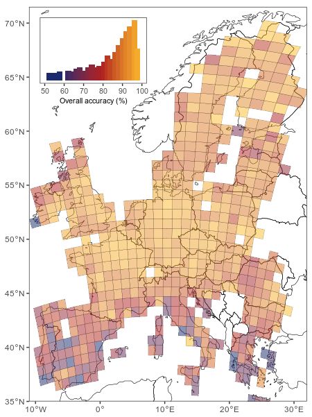
Continental-Scale Land Cover Mapping at 10 m Resolution over Europe (ELC10)
Remote
 RemoteSens.  2021,13,
        Sens.2021,  13,2301
                        x FOR PEER REVIEW                                                                                                                       4 of2322
                                                                                                                                                              4 of

      Figure1.1.Study
     Figure      Studyarea
                        areawith
                              withavailable
                                   availableland
                                             landcover
                                                  coverreference
                                                         referencepoints
                                                                    points(A)
                                                                           (A)and
                                                                                andSentinel
                                                                                     Sentinel(B,C)
                                                                                               (B,C)satellite
                                                                                                       satelliteimagery.
                                                                                                                 imagery.Each
                                                                                                                          Eachpoint
                                                                                                                                pointinin(A)
                                                                                                                                          (A)is
     aissampling
          a sampling location
                  location     (53,476
                           (53,476     polygons
                                    polygons  andand  282,854
                                                   282,854     points)
                                                            points)    with
                                                                    with      a land
                                                                          a land      cover
                                                                                   cover     class
                                                                                         class     label.
                                                                                                label.  TheThe   number
                                                                                                             number      of available
                                                                                                                     of available     cloud‐
                                                                                                                                   cloud-free
      free Sentinel‐2
     Sentinel-2  pixelspixels
                        and Sentinel-1  pixelspixels
                              and Sentinel‐1   duringduring
                                                       2018 2018  are mapped
                                                             are mapped    in (B)inand
                                                                                    (B) and  (C), respectively.
                                                                                        (C), respectively.

                                     2.2. Land Cover Reference Data
                                    2.2.
                                            LUCAS is a European Union
                                           LUCAS                             Union initiative
                                                                                         initiative toto gather
                                                                                                         gather in  insitu
                                                                                                                        situground‐truth
                                                                                                                                ground-truthdata      dataon   onland
                                                                                                                                                                    land
                                     cover over
                                    cover    over 27 member states and          and is is updated
                                                                                           updated every
                                                                                                       everythree
                                                                                                               threeyears
                                                                                                                        years[29]. [29].ItItexcludes
                                                                                                                                               excludesNorway,Norway,
                                     Switzerland, Liechtenstein,
                                    Switzerland,      Liechtenstein,and     andthe thenon-EU
                                                                                         non‐EU Balkan
                                                                                                    Balkan states.
                                                                                                              states. Each
                                                                                                                       Each iteration
                                                                                                                                 iteration includes
                                                                                                                                                includes visiting
                                                                                                                                                              visitinga
                                     a sub‐sample
                                    sub-sample         of the
                                                    of the       1,090,863
                                                            1,090,863            geo‐referenced
                                                                          geo-referenced         pointspoints
                                                                                                          withinwithin      the LUCAS
                                                                                                                    the LUCAS           2 km 2point
                                                                                                                                                  km point        grid.
                                                                                                                                                         grid. Under
                                     Under    the  2018  LUCAS        Copernicus          module,    58,428   of  the  point
                                    the 2018 LUCAS Copernicus module, 58,428 of the point locations have been quality assured     locations      have    been    qual‐
                                     ity assured
                                    and             and transformed
                                           transformed      into polygons    intoof  polygons
                                                                                        homogenousof homogenous
                                                                                                           land cover    land    cover specifically
                                                                                                                             specifically       tailored tailored
                                                                                                                                                             for earth
                                     for  earth  observation       (Figure       2).  The   polygons     are  approximately
                                    observation (Figure 2). The polygons are approximately 0.5 ha in size and are                      0.5   ha   in size    and are
                                                                                                                                                       therefore      (by
                                     therefore
                                    design)      (byenough
                                              large   design)so   large
                                                                    that enough
                                                                           at least one so that  at least
                                                                                            Sentinel   10 ×one10Sentinel
                                                                                                                 m pixel is10contained
                                                                                                                                    × 10 m pixel fullyiswithin
                                                                                                                                                         contained them
                                     fullysome
                                    with    within   themfor
                                                  space      with    some space
                                                                registration           forWe
                                                                                   error.   registration
                                                                                                used the error.
                                                                                                            collated Weand used     the collated
                                                                                                                                cleaned               and cleaned
                                                                                                                                             Copernicus        Module
                                     Copernicus
                                    polygon          Module
                                                dataset   (n = polygon        dataset (n
                                                                 53,476) provided           by= d’Andrimont
                                                                                                53,476) provided   et al.by[25].
                                                                                                                              d’Andrimont
                                                                                                                                    The centroid    et al.  [25].of
                                                                                                                                                       points      Thethe
                                     centroid points
                                    Copernicus      Moduleof the   Copernicus
                                                                polygons               Module
                                                                               (hereafter         polygons
                                                                                              referred   to as (hereafter
                                                                                                                LUCAS polygon   referredcentroids)
                                                                                                                                              to as LUCAS  werepol‐used
                                     ygon
                                    as  the centroids)
                                             core of ourwere      used as
                                                            reference          the core
                                                                          sample       for of  ourcover
                                                                                            land    reference    sample for
                                                                                                           classification.      Theland     cover classification.
                                                                                                                                       top-level     of the LUCAS
                                     The   top‐level   of  the  LUCAS        land     cover   typology     was  used     in
                                    land cover typology was used in the present analysis including artificial land, cropland, the   present      analysis     includ‐
                                     ing  artificial land,   cropland,       woodland,        shrubland,
                                    woodland, shrubland, grassland, bare land, wetland and water (Table 1).  grassland,       bare    land,    wetland       and   wa‐
                                     ter (Table
                                           After 1).
                                                   establishing baseline land cover proportions using the CORINE land cover
                                    dataset After  establishing
                                               (re-coded      to our baseline
                                                                       typology)   landas  cover   proportions
                                                                                             a reference     [12], using
                                                                                                                     we found the CORINE
                                                                                                                                      that theland         cover da‐of
                                                                                                                                                    distribution
                                     tasetLUCAS
                                    the     (re‐coded    to our typology)
                                                     polygons        were biased     as atoward
                                                                                           reference    [12], weand
                                                                                                     cropland       found      that the distribution
                                                                                                                           woodland           land cover classesof the
                                     LUCASS1).
                                    (Figure     polygons     were biased
                                                     Consequently,        there   toward
                                                                                    were verycropland    and woodland
                                                                                                   few LUCAS         polygons    landforcover
                                                                                                                                           water,  classes
                                                                                                                                                     wetland, (Figure
                                                                                                                                                                    bare
                                     S1). Consequently,
                                    land    and artificial landthereclasses
                                                                        were very  (FigurefewS1).
                                                                                                LUCAS      polygons performed
                                                                                                     We therefore         for water, wetland,             bare landof
                                                                                                                                             a bias correction
                                     andreference
                                    the    artificial land
                                                       sample classes   (Figure
                                                                   (Figure      2) by S1).using
                                                                                            We therefore      performed
                                                                                                  the harmonised          LUCASa biastheoretical
                                                                                                                                          correction of       thepoint
                                                                                                                                                           grid    ref‐
                                     erence   sample    (Figure     2) by   using     the  harmonised       LUCAS      theoretical
                                    (hereafter LUCAS points) data [24] to supplement the LUCAS polygon centroid dataset so                grid   point    (hereafter
                                     LUCAS
                                    that        points)reference
                                          the overall     data [24] sample
                                                                        to supplement          the LUCASofpolygon
                                                                                     was representative           the CORINE  centroid       dataset soAlthough
                                                                                                                                        proportions.         that the
                                     overall
                                    the   LUCASreference     samplepoints
                                                     theoretical        was representative
                                                                                   have not beenoftransformed
                                                                                                          the CORINEinto       proportions.
                                                                                                                                     polygons,Althoughthey are the   still
                                     LUCAS theoretical
                                    appropriate      for earth points     have notapplications
                                                                   observation           been transformed         intoapplying
                                                                                                         [15] after      polygons,certain  they are     still appro‐
                                                                                                                                                    quality     control
                                     priate for earth
                                    procedures.          observation
                                                     We employed         theapplications        [15] after
                                                                                metadata filtering           applying
                                                                                                         (Figure           certain in
                                                                                                                    2) outlined        quality
                                                                                                                                           Weigand  control
                                                                                                                                                         et al.proce‐
                                                                                                                                                                 [26] to
                                     dures.
                                    filter    We
                                            out     employed
                                                points   where the the metadata
                                                                         land coverfiltering         (Figure
                                                                                           parcel area   was 2)
Continental-Scale Land Cover Mapping at 10 m Resolution over Europe (ELC10)
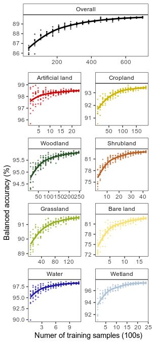
Remote Sens. 2021, 13, 2301                                                                                                           5 of 22

                              Table 1. Land cover typology adopted along with LUCAS codes and descriptions.

   Land Cover Label                             LUCAS Class Definitions and Sub-Class Inclusions and Exclusions
                              Artificial land (A00): Areas characterised by an artificial and often impervious cover of constructions and
                              pavement. Includes roofed built-up areas and non-built-up area features such as parking lots and yards.
      Artificial land         Excludes non-built-up linear features such as roads, and other artificial areas such as bridges and viaducts,
                              mobile homes, solar panels, power plants, electrical substations, pipelines, water sewage plants, open
                              dump sites.
                              Cropland (B00): Areas where seasonal or perennial crops are planted and cultivated, including cereals, root
                              crops, non-permanent industrial crops, dry pulses, vegetables, and flowers, fodder crops, fruit trees and
        Cropland
                              other permanent crops. Excludes temporary grasslands which are artificial pastures that may only be
                              planted for one year.
                              Woodland (C00): Areas with a tree canopy cover of at least 10% including woody hedges and palm trees.
        Woodland              Includes a range of coniferous and deciduous forest types. Excludes forest tree nurseries, young
                              plantations or natural stands (5 m of height. It may include sparsely occurring trees with a canopy below 10%.
                              Excludes berries, vineyards and orchards.
                              Grassland (E00): Land predominantly covered by communities of grassland, grass-like plants and forbs.
                              This class includes permanent grassland and permanent pasture that is not part of a crop rotation
                              (normally for 5 years or more). It may include sparsely occurring trees within a limit of a canopy below
                              10% and shrubs within a total limit of cover (including trees) of 20%. This may include: dry grasslands; dry
                              edaphic meadows; steppes with gramineae and artemisia; plain and mountainous grassland; wet
        Grassland
                              grasslands; alpine and subalpine grasslands; saline grasslands; arctic meadows; set aside land within
                              agricultural areas including unused land where revegetation is occurring; clear cuts within previously
                              existing forests. Excludes spontaneously re-vegetated surfaces consisting of agricultural land which has
                              not been cultivated this year or the years before; clear-cut forest areas; industrial “brownfields”;
                              storage land.
                              Bare land and lichens/moss (F00): Areas with no dominant vegetation cover on at least 90% of the area or
        Bare land             areas covered by lichens/ moss. Excludes other bare soil, which includes bare arable land, temporarily
                              unstocked areas within forests, burnt areas, secondary land cover for tracks and parking areas/yards.
                              Water areas (G00): Inland or coastal areas without vegetation and covered by water and flooded surfaces,
          Water               or likely to be so over a large part of the year. Additionally, includes areas covered by glaciers or
                              permanent snow.
                              Wetlands (H00): Wetlands located inland and having fresh water. Additionally, wetlands located on
         Wetland
                              marine coasts or having salty or brackish water, as well as areas of a marine origin.

                                           The outlier ranking procedure involved extracting Sentinel-2 data (see Section 2.3. for
                                     details) for pixels intersecting LUCAS points. These were fed into a random forest (RF)
                                     classification model (see Section 2.5 for details) which was used to calculate classification
                                     uncertainty for each LUCAS point. The RF model iteratively selects a random subset of
                                     data to generate decision trees which are validated against the withheld data. During
                                     each iteration, the model generates votes for the most likely class label. We extracted the
                                     fraction of votes for the correct land cover class at each LUCAS point after bootstrapping
                                     the RF procedure 100 times. We acknowledge that this bootstrapping of the RF model
                                     itself may not be necessary, however, it may smooth over any artifacts introduced from the
                                     internal bootstrapping of a single RF model. LUCAS points with a high fraction of votes
                                     (close to 1) can be considered as archetypal instances of the given land cover class, whereas
                                     those with a low fraction of votes (close to 0) are considered as mislabelled or spectrally
                                     contaminated. We ranked the LUCAS points by their fraction of correct votes and selected
                                     the topmost points for each land cover class to supplement the LUCAS polygon centroids
                                     so that the final land cover proportions matched that of the CORINE dataset. The number
                                     of supplemental LUCAS points needed (n = 18,009) was determined as relative to the most
                                     abundant LUCAS polygon class (cropland in Figure S1).
Remote Sens. 2021, 13, x FOR PEER REVIEW                                                                                                5 of 23

Remote Sens. 2021, 13, 2301             supplement the LUCAS polygon sample. Of these, 18,009 LUCAS points were selected6 of 22
                                        following an outlier ranking procedure to remove mislabelled or contaminated LUCAS
                                        points.

           Figure
      Figure      2. Methodological
             2. Methodological      workflow
                                workflow    forfor evaluatingthe
                                                evaluating    thepre-processing
                                                                  pre‐processing of
                                                                                  ofdecisions
                                                                                    decisionsiningenerating
                                                                                                  generatingthethe
                                                                                                                final ELC10
                                                                                                                   final    landland
                                                                                                                          ELC10  covercover
           map. Underlined  outcomes  are those  that were  chosen for the final model. Abbreviations:  S1—sentinel   1;
      map. Underlined outcomes are those that were chosen for the final model. Abbreviations: S1—sentinel 1; S2—sentinel S2—sentinel 2; 2;
           Aux vars—auxiliary variables.
      Aux vars—auxiliary variables.
                               Table 1. Land cover typology adopted along with LUCAS codes and descriptions.
                                    2.3. Sentinel Spectro-Temporal Features
        Land Cover Label                    AllLUCAS
                                                 remote Class
                                                           sensing   analyses were
                                                                  Definitions            conducted
                                                                                   and Sub‐Class          in the Google
                                                                                                       Inclusions           Earth Engine cloud comput-
                                                                                                                      and Exclusions
                                     ing platform for geospatial analysis [6]. We processed all Sentinel-2 optical and Sentinel-1
                               Artificial  land (A00):
                                     synthetic            Areas
                                                   aperture       characterised
                                                                radar   (SAR) scenesby anover
                                                                                            artificial
                                                                                                   Europeand often
                                                                                                               duringimpervious
                                                                                                                         2018. Thiscover   of con‐ to a total
                                                                                                                                       amounts
                               structions   and pavement.
                                     of 239,818                 Includes
                                                    satellite scenes        roofedwould
                                                                         which       built‐up    areas and
                                                                                             typically         non‐built‐up
                                                                                                            require   approx.area700features   such space
                                                                                                                                      TB storage     as    if
          Artificial land      parking
                                     not lots
                                          for and
                                               Googleyards.  Excludes
                                                          Earth   Engine non‐built‐up
                                                                             and cloud linear       features such
                                                                                           computation.         The as   roads, satellite
                                                                                                                     Sentinel    and otherdata
                                                                                                                                             artificial
                                                                                                                                                  were used
                               areastosuch   as bridges
                                        derive             and viaducts,features
                                                   spectro-temporal          mobile homes,       solar panels,
                                                                                       as predictor              power
                                                                                                          variables        plants,
                                                                                                                       in our  landelectrical  substa‐
                                                                                                                                      cover classification
                               tions,model.
                                      pipelines,    water sewage plants,
                                                 Spectro-temporal               openwere
                                                                         features     dumpused  sites.to capture both the spectral and temporal
                                     (e.g., phenology or crop cycle) characteristics of land cover classes and offer enhanced
                               Cropland (B00): Areas where seasonal or perennial crops are planted and cultivated, including
                                     model prediction accuracy compared to single time-point image classification [15,30]. To
                               cereals, root crops, non‐permanent industrial crops, dry pulses, vegetables, and flowers, fodder
             Cropland                generate model training data, spectro-temporal metrics were extracted for Sentinel pixels
                               crops, fruit trees and other permanent crops. Excludes temporary grasslands which are artifi‐
                                     intersecting the LUCAS points, or the centroids of the LUCAS polygons.
                               cial pastures that may only be planted for one year.
                                            Sentinel-2 images for both Top of Atmosphere (TOA; Level 1C) and Surface Reflectance
                               WoodlandLevel-2A)
                                     (SR;     (C00): Areas were
                                                              withused
                                                                    a treeto   test the
                                                                            canopy    covereffect
                                                                                              of atof    atmospheric
                                                                                                     least   10% including correction    on classification
                                                                                                                               woody hedges      and
                               palm trees. Includes a range of coniferous and deciduous forest types. Excludes forestthan
                                     accuracies     (Q1  in  Figure   2).  The   scenes   were    first  filtered  for  those  with   less   tree 60% cloud
            Woodland                 coveryoung
                                              (129,839    removed
                               nurseries,            plantations    or of  280,420
                                                                       natural        scenes)
                                                                                  stands   (< 10% using
                                                                                                     canopythe cover),
                                                                                                                “CLOUDY_PIXEL_PERCENTAGE”
                                                                                                                         dominated by shrubs or
                               grass.scene     metadata     field.  We    then    performed       a  pixel-wise     cloud masking procedure using
                                     the cloud probability score produced by the S2cloudless algorithm [31]. S2cloudless is a
                                     machine
                               Shrubland          learning-based
                                             (D00):   Areas dominated  algorithm
                                                                             (at leastand
                                                                                       10%is ofpart    of the latest
                                                                                                 the surface)           generation
                                                                                                                 by shrubs    and lowofwoody
                                                                                                                                          cloud detection
            Shrubland          plants  normally not
                                     algorithms      for able  to reach
                                                         optical   remote >5 m   of height.
                                                                              sensing         It mayAfter
                                                                                         images.        include  sparsely
                                                                                                              visually       occurringthe
                                                                                                                         inspecting      trees  withmasking
                                                                                                                                            cloud     a
                               canopy    below
                                     results      10%. Excludes
                                                across  a range of  berries,   vineyards
                                                                       Sentinel-2           andwe
                                                                                      scenes,      orchards.
                                                                                                      settled on a cloud probability threshold of
                                     40% for our masking procedure. After cloud masking and mosaicking two years’ worth
                               Grassland     (E00): Land
                                     of Sentinel-2          predominantly
                                                        scenes,                 covered
                                                                   the cloud-free          by communities
                                                                                        pixel    availability of    grassland,
                                                                                                                  ranged     from grass‐like
                                                                                                                                    less than plants
                                                                                                                                                 10 to over
            Grassland          and forbs.   This   class includes    permanent
                                    100 pixels over the study area (Figure 1B).     grassland     and   permanent      pasture  that is not  part of a
                               crop rotationUsing(normally    for 5 years or more).
                                                     the cloud-masked                   It may
                                                                                Sentinel-2        include sparsely
                                                                                               imagery,       we derivedoccurring   trees within
                                                                                                                              the median           a of all
                                                                                                                                              mosaic
                                     spectral bands. The median mosaic was derived by calculating the pixel-wise median value
                                     across the time series of images within the year. In addition, we calculated the following
                                     spectral indices for each cloud-masked scene: normalised difference vegetation index [32],
                                     normalised burn ratio [33], normalised difference built index [34], and normalised differ-
                                     ence snow index [35]. For each spectral index, we used the temporal resolution to calculate
                                     the 5th, 25th, 50th, 75th and 95th percentile mosaics as well as the standard deviation, kurto-
                                     sis and skewness across the two-year time stack of imagery. We derived the median NDVI
                                     values for the summer (June–August), winter (December–February), spring (March–May),
Remote Sens. 2021, 13, 2301                                                                                            7 of 22

                              and fall (September–November). The spectro-temporal metrics described above have been
                              extensively used to map land cover and land use changes with optical remote sensing [36].
                              Finally, several studies have found that textural image features (i.e., defining pixel values
                              from those of their neighbourhood) for Sentinel-2 imagery significantly enhanced land
                              cover classification accuracy [26,37]. Therefore, we calculated the standard deviation of
                              median NDVI within a 5 × 5 pixel moving window.
                                   Sentinel-1 SAR Ground Range Detected data were pre-processed by Google Earth
                              Engine, including thermal noise removal, radiometric calibration and terrain correction
                              using global digital elevation models. Sentinel-1 scenes were filtered for interferometric
                              wide swath and a resolution of 10 m to suit our land cover classification purposes. We
                              performed an angular-based radiometric slope correction using the methods outlined in
                              Vollrath et al. [38]. SAR data can contain a substantial speckle and backscatter noise which
                              is important to address particularly when performing pixel-based image classification.
                              We applied a Lee-sigma speckle filter [39] to the Sentinel-1 imagery to test the effect on
                              classification accuracy (Q2 Figure 2). Following pre-processing, we calculated the median
                              and standard deviation mosaics for the time stacks of imagery including the single co-
                              polarised, vertical transmit/vertical receive (VV) band and the cross-polarised, vertical
                              transmit/horizontal receive (VH) band, as well as the ratio between them (VV/VH).

                              2.4. Auxiliary Features
                                    A challenge of classifying regional-scale land cover is that models relying on spectral
                              responses alone may be limited by the fact that land cover characteristics can change drasti-
                              cally between climate and vegetation zones. For example, a grassland in the Mediterranean
                              will have very different spectro-temporal signatures to a grassland in the boreal zone.
                              Previous regional land cover classification efforts have dealt with this by either (1) splitting
                              the area up into many small parts and running multiple classification models [20], or (2)
                              including environmental covariates that help the model explain the regional variation
                              in land cover characteristics [15,40]. We tested the latter approach (Q4 in Figure 2) by
                              including a range of environmental auxiliary covariates into our classification model.
                                    Auxiliary variables included elevation data from the Shuttle Radar Topography Mis-
                              sion (SRTM) digital elevation dataset [41] at 30 m resolution which covers up to 60◦ north.
                              For higher latitudes, we used the 30 arc-second elevation data from the United States
                              Geological Survey (GTOPO30). Climate data were derived from the ERA5 fifth genera-
                              tion ECMWF atmospheric reanalysis of the global climate [42]. We used it to calculate
                              the 10-year (2010–present) average and standard deviation in monthly precipitation and
                              temperature at 25 km resolution. Finally, we also included data on night-time light sources
                              at approx. 500 m spatial resolution. This was intended to assist the model in differentiating
                              artificial surfaces and bare ground in alpine areas. A median 2018 radiance composite
                              image from the Visible Infrared Imaging Radiometer Suite (VIIRS) Day/Night Band (DNB),
                              provided by the Earth Observation Group, Payne Institute, was used [43].

                              2.5. Classification Models and Accuracy Assessment
                                    The land cover classification model evaluation and tuning were conducted in R with
                              the ‘randomForest’ and ‘caret’ packages (R Core Team, 2019), while the final model infer-
                              ence over Europe was conducted in Google Earth Engine using equivalent model parame-
                              ters. We chose an ensemble learning method, namely the random forest (RF) classification
                              model. RF deals well with large and noisy input data, accounts for non-linear relationships
                              between explanatory and response variables, and is robust against overfitting [44]. A
                              recent review of land cover classification literature found that the RF algorithm has the
                              highest accuracy level in comparison with the other classifiers adopted [45]. Classification
                              accuracies were determined using internal randomised cross-validation procedures where
                              error rates are determined from the mean prediction error on each training sample xi ,
                              only using the trees that did not have xi in their bootstrap sample (i.e., out-of-bag; [46]).
                              Predicted and observed land cover classes are used to build a confusion matrix from which
Remote Sens. 2021, 13, 2301                                                                                            8 of 22

                              one derives overall accuracy (OA), user’s accuracy (UA), and producer’s accuracy (PA).
                              See Stehman and Foody [47] for details.
                                    A series of RF models were run at each step in the pre-processing tests (Figure 2) in
                              order to assess the effect of pre-processing decisions on classification accuracy. With each
                              consecutive step, we chose the pre-processing option that yielded the highest accuracy
                              to generate the data for the subsequent step. The final pre-processing sequence that led
                              to the final RF model data were indicated by the underlined decisions in Figure 2. When
                              testing the effect of reference sample size (Q6 in Figure 2), we iteratively removed 5% of the
                              training dataset and assessed model performance. All 71,485 LUCAS locations (polygon
                              centroids and theoretical points) were used to train the final RF model. At this stage we
                              performed recursive feature elimination which is a process akin to backward stepwise
                              regression that prevents overfitting and reduces unnecessary computational load [48].
                              Recursive feature elimination produces a model with the maximum number of features
                              and iteratively removes the weaker variables until a specified number of features is reached.
                              In our case, this was 15 features. The top predictor variables were selected based on the
                              variable importance ranking using both the mean decrease in accuracy and mean decrease
                              in Gini coefficient scores [49]. Finally, we also tuned the RF hyperparameters by iterating
                              over a series of ntree (50 to 500 in 25 tree intervals) and mtry (1 to 10) and found the optimal
                              (based on lowest model error rate) combination of settings to include a ntree of 100 and
                              mtry set to the square root of the number of covariates (3.8).
                                    Part of enhancing the usability of land cover maps is quantifying the spatial distribu-
                              tion of classification uncertainty. There are methods to derive pixel-based and sample-based
                              uncertainty estimates that are spatially explicit [37,50,51]. We adopted a sample-based
                              uncertainty estimate by dividing the study area into 100 km equal-area grid squares de-
                              fined by the European Environmental Agency reference grid. For each grid cell, we use
                              our final trained RF model to make predictions against the LUCAS reference data within
                              and build a confusion matrix to derive overall accuracy for the grid cell in question. We
                              acknowledge that making predictions over reference samples that were included in model
                              training is likely to inflate accuracy estimates. However, in this case, we are interested in
                              obtaining the relative distribution of accuracy over the study region to give insight into
                              class non-separability and map reliability over space.

                              2.6. Comparison with Other Land Cover Maps
                                   We compared our land cover product with two other global land cover products
                              including CORINE [12], and FROM-GLC10 [23], and two other European land cover maps
                              including the map created by Pflugmacher et al. [15] and S2GLC [14]. The CORINE map
                              was updated for 2018 at 100 m resolution by the Copernicus Land Management Service
                              and is widely used for aerial statistics and accounting. FROM-GLC10 is a global map
                              produced with Sentinel satellite data at 10 m resolution. The S2GLC (Sentinel-2 Global
                              Land Cover) map has been produced over Europe during 2017 using Sentinel 2 data at
                              10 m resolution. The Pflugmacher et al. [15] map was produced for 2015 using Landsat
                              data at 30 m resolution. All land cover typologies were converted to the LUCAS typology
                              used in our analysis for purposes of comparison (Table S1). The same accuracy assessment
                              protocols described above were used to assess the accuracy of these maps using the same
                              validation dataset (completely withheld from the training of our model).
                                   Apart from assessing the classification accuracy, we tested the utility of the maps for
                              calculating aerial land cover statistics over spatial units defined for the European Union by
                              the nomenclature of territorial units (NUTS). We used NUTS level 2 basic regions which
                              include population sizes between 0.8 and 3 million and are used for the application of
                              regional policies. Area proportions for each land cover class and map product, including
                              ELC10, were calculated for each of the NUTS polygons. Within each NUTS polygon,
                              we also calculated the area proportions using the original LUCAS survey dataset. We
                              regressed the mapped area proportions on the area proportions estimated from the LUCAS
                              sample to assess the land cover map’s utility for land cover accounting. Although the
Remote Sens. 2021, 13, 2301                                                                                                                     9 of 22

                                  statistics derived from LUCAS dataset also have uncertainty associated with them, they
                                  are considered the only harmonised dataset for area statistics in Europe and were therefore
                                  used as the benchmark with which we compared the land cover maps.

                                  3. Results
                                  3.1. Effects of Satellite Data Pre-Processing
                                              The pre-processing of Sentinel optical and radar imagery had very little effect on the over-
                                        all classification accuracy (Figure 3A,B). Specifically, the atmospheric correction of Sentinel-2
                                        and speckle filtering of Sentinel-1 imagery enhanced the classification accuracy by less than 1%
                                        compared to models with TOA and non-speckle filtered imagery, respectively. This marginal
                                        difference was true for all class-specific accuracies (Figure S2). However, the fusion of Sentinel-
                                       1 and Sentinel-2 data within a single model increased accuracy by 3% compared to Sentinel-2
                                        alone and by 10% compared to Sentinel-1 alone (Figure 3C). Class-specific accuracies reveal
                                        that models with Sentinel-1 data alone perform particularly badly when predicting wetland,
                                        shrubland and bare land classes (Figure S2c). In these instances, fusing both optical and radar
                                        data increases accuracy by up to 30% compared to Sentinel-1 data alone. The addition of
                                        auxiliary data (terrain, climate and night-time lights) increased accuracy by an additional 2%
                                        compared to a model with Sentinel data alone (Figure 3D). Auxiliary data
  Remote Sens. 2021, 13, x FOR PEER REVIEW                                                                           10 of have
                                                                                                                           23   the largest
                                        benefits for bare land and shrubland classes (Figure S2d).

                                   Figure
                                Figure      3. The
                                        3. The effecteffect  of pre-processing
                                                      of pre‐processing  decisionsdecisions   on land
                                                                                   on land cover         cover classification
                                                                                                  classification                 accuracy. The random
                                                                                                                  accuracy. The random
                                forest model
                                   forest     overall
                                           model       accuracies
                                                   overall        are displayed
                                                             accuracies          for alternative
                                                                          are displayed          Sentinel 2 (A),
                                                                                           for alternative       and 1 (B)
                                                                                                              Sentinel     pre‐pro‐
                                                                                                                        2 (A), and 1 (B) pre-processing
                                cessing steps, Sentinel 1 and 2 data fusion options (C), the addition of auxiliary variables (D), and
                                   steps, Sentinel 1 and 2 data fusion options (C), the addition of auxiliary variables (D), and the quality
                                the quality of reference data (E). Each panel corresponds to a pre‐processing decision in the work‐
                                   of outlined
                                flow  reference   data (E).
                                               in Figure      Each
                                                          2. The    panel
                                                                 option    corresponds
                                                                        with               to a pre-processing
                                                                              the highest accuracy                  decision
                                                                                                    is utilised in the        in the
                                                                                                                       proceeding     workflow outlined
                                                                                                                                   step.
                                   in Figure 2. The option with the highest accuracy is utilised in the proceeding step.
                                3.2. Effects of Reference Data Pre‐Processing
                                     The first test of reference data pre‐processing was a test of quality checking and clean‐
                                ing the LUCAS data via the conversion of LUCAS points into homogenous polygons un‐
                                der the Copernicus module (Figure 2). Extracting the satellite data at LUCAS points vs.
                                the centroids of homogenous LUCAS polygons increased accuracy by less than 1% (Figure
Remote Sens. 2021, 13, 2301                                                                                                            10 of 22

                                   3.2. Effects of Reference Data Pre-Processing
                                            The first test of reference data pre-processing was a test of quality checking and clean-
                                       ing the LUCAS data via the conversion of LUCAS points into homogenous polygons under
                                       the Copernicus module (Figure 2). Extracting the satellite data at LUCAS points vs. the
                                       centroids of homogenous LUCAS polygons increased accuracy by less than 1% (Figure 3E).
                                       This marginal effect was evident for all class-specific accuracy scores (Figure S2e). The
                                       second test related to reference data involved the iterative depletion of the sample size. The
                                       relationship between sample size and overall accuracy appears to follow an exponential
                                       plateau curve (Figure 4). The benefit to model accuracy gained by increasing sample size
                                       depletes so rapidly that, for example, when one increases from 5K to 20K points, accuracy
                                       increases by 0.15% per 1K points added, while when one increases from 55K 11
   Remote Sens. 2021, 13, x FOR PEER REVIEW                                                                                 to of
                                                                                                                               70K23 points,
                                       accuracy increases by 0.015% per 1K points. Therefore, the difference between 5K and
                                       50K LUCAS points is only 3% (86% vs. 89%; Figure 4). The same pattern is evident for
                                       class-specific
                                      from            accuracies.
                                            the bootstrapped       However, it isincreased
                                                               RF classifications importantasto
                                                                                              thenote that the
                                                                                                  number       variance
                                                                                                           of training   in accuracy
                                                                                                                       samples  de‐ from
                                       the bootstrapped RF classifications increased as the number of training samples decreased.
                                      creased.

                                  Figure
                                  Figure4.4.The
                                              Theeffect ofof
                                                   effect thethe
                                                              reference sample
                                                                 reference      size size
                                                                           sample    on overall and class‐specific
                                                                                          on overall               accuracy.
                                                                                                     and class-specific       The random
                                                                                                                          accuracy.  The random
                                  forest classification models  were trained on iteratively smaller sample  sizes. Points in each facet
                                  forest classification models were trained on iteratively smaller sample sizes. Points in each facet plot
                                  plot represent bootstrapped (n = 10) model accuracy estimates and are fit with Loess regression
                                  represent bootstrapped (n = 10) model accuracy estimates and are fit with Loess regression lines.
                                  lines.

                                  3.3. ELC10 Final Accuracy Assessment
                                       The final RF classification model produced an overall accuracy of 90.2% across eight
                                  land cover classes (Table 2). The class‐specific user’s accuracy (UA; errors of commission)
most often confused with grassland and woodland probably due to the spectral similarity
                                   across a gradient of woody plant cover. Similarly, cropland was most often confused with
                                   grassland probably due to the temporal similarity in spectral signatures between mowed
                                   pastures and ploughed fields.
Remote Sens. 2021, 13, 2301                                                                                                     11 of 22
      Table 2. Estimated error matrix for the final classification with estimates for user’s accuracy (UA) and producer’s accuracy
      (PA). Overall accuracy is 90.2%.

                               Reference
                                   3.3. ELC10 Final Accuracy Assessment
        Prediction              1        2 final 3RF classification
                                         The                   4         5
                                                                      model      6
                                                                              produced    7 overall8accuracy
                                                                                         an                 Total     UA
                                                                                                               of 90.2%    (%) eight
                                                                                                                         across  SE
1      Artificial land        2339 land57           8 (Table222). The class-specific
                                         cover classes                   3       0        0 accuracy
                                                                                      user’s        4 (UA;2433          96.1     0.4
                                                                                                              errors of commission)
2        Bare land             15 describes
                                       1219 the reliability
                                                    5         43        54 and informs
                                                               of the map       19        7 user of
                                                                                         the       17 how well
                                                                                                             1379the map88.4     0.8
                                                                                                                          represents
3       Cropland               13 what    is really
                                        124          on the ground.
                                                16,251       931       UA exhibited
                                                                       190       0     a 11
                                                                                          wide range
                                                                                                  172 from17,692
                                                                                                              75% for shrubland
                                                                                                                        91.9     0.2to
4       Grassland              19 96.4% 118for woodland.
                                                 1171       The relative
                                                            13,378     499decrease
                                                                                 5 in prediction
                                                                                         62       accuracy15,694
                                                                                                  442        over shrubland
                                                                                                                        85.2 classes
                                                                                                                                 0.3
5       Shrubland               6  is evident
                                        120    in the
                                                  207  spatial distribution
                                                             255      3002  of model
                                                                                 0    errors
                                                                                          5   (Figure
                                                                                                  404  5). The  majority
                                                                                                             3999        of the error
                                                                                                                        75.1     0.7
6          Water                0 (accuracies
                                        20      below
                                                    1 80%) was 5 distributed
                                                                         0     over southern
                                                                               1110      15 Europe  2 where    shrubland
                                                                                                             1153         dominates
                                                                                                                        96.3     0.5
7        Wetland                0 (Figure
                                        48 1A). Conversely,
                                                   11         28model accuracies
                                                                        24       2 were   highest (above
                                                                                       2379        59      90%)
                                                                                                             2551over the interior
                                                                                                                        93.3     0.5of
                                   Europe (Figure 5) where cropland and woodland dominate (Figure 1A). Shrubland was
8       Woodland                6       126       280        502       719       2       23     23,288      24,946      93.4     0.2
                                   most often confused with grassland and woodland probably due to the spectral similarity
           Total              2398     1832     17,934      15,164    4491 1138 2502            24,388      69,847
                                   across a gradient of woody plant cover. Similarly, cropland was most often confused with
          PA (%)              97.5     66.5       90.6       88.2      66.8    97.5     95.1     95.5                   90.2
                                   grassland probably due to the temporal similarity in spectral signatures between mowed
             SE                0.9 pastures
                                        0.6 and 0.2           0.3
                                                   ploughed fields.     0.7     0.3      0.7      0.1                            0.1

                                   Figure 5. Map showing land cover classification accuracy over 100 × 100 km grid squares. The inset
                                   bar plot shows the abundance of grid squares across the range of error (percentage overall accuracy).
                                   Missing grid cells are where there were insufficient validation samples to construct an error matrix.

                                         Sentinel optical variables were the two most important covariates in the final RF
                                   model (Figure 6). The first and fifth most important variables were the 25th percentile of
                                   NDVI and standard deviation in NBR over time, respectively. These metrics both capture
                                   the temporal dynamics of spectral responses that are important in distinguishing land
                                   cover classes such as cropland and grassland. The Sentinel 1 VH band also exhibited a
                                   relatively high importance score. Of the auxiliary variables, night-time light intensity and
                                   temperature were the most important variables.
Remote Sens. 2021, 13, 2301                                                                                                             12 of 22

          Table 2. Estimated error matrix for the final classification with estimates for user’s accuracy (UA) and producer’s accuracy
Remote Sens. 2021, 13, x FOR PEER REVIEW                                                                                        13 of 23
          (PA). Overall accuracy is 90.2%.

                                 Reference
           Prediction            1    Figure2 5. Map showing
                                                      3        land4 cover classification
                                                                             5          6 accuracy
                                                                                                 7 over 100 8 × 100 km grid squares.
                                                                                                                     Total     UA (%)The in‐SE
                                      set bar plot shows the abundance of grid squares across the range of error (percentage overall ac‐
             Artificial
      1                     2339           57 Missing
                                      curacy).        8 grid cells22
                                                                   are where3there were 0 insufficient
                                                                                                 0          4
                                                                                                       validation    2433 to construct
                                                                                                                  samples       96.1 an 0.4
               land
      2     Bare land            15   error  matrix.
                                          1219        5           43        54         19        7         17        1379       88.4        0.8
      3     Cropland             13      124      16,251      931       190       0       11       172    17,692       91.9       0.2
      4     Grassland            19        Sentinel1171
                                         118        optical variables
                                                             13,378    were
                                                                        499 the 5two most 62 important
                                                                                                   442 covariates
                                                                                                          15,694 in the85.2final RF
                                                                                                                                  0.3
      5     Shrubland             6   model
                                         120 (Figure
                                                   2076). The first
                                                              255 and 3002
                                                                        fifth most0 important
                                                                                           5 variables       the 25th percentile
                                                                                                   404 were3999        75.1       of
                                                                                                                                  0.7
      6       Water               0   NDVI20 and standard
                                                    1           5
                                                            deviation in 0NBR over
                                                                                1110time, respectively.
                                                                                          15        2 These1153        96.3 capture
                                                                                                             metrics both         0.5
      7      Wetland              0   the 48
                                          temporal 11dynamics28of spectral
                                                                         24 responses
                                                                                  2     2379are important
                                                                                       that        59      2551
                                                                                                          in           93.3
                                                                                                              distinguishing      0.5
                                                                                                                               land
      8     Woodland              6      126       280        502       719       2       23     23,288   24,946       93.4       0.2
                                      cover classes such as cropland and grassland. The Sentinel 1 VH band also exhibited a
              Total         2398         1832
                                      relatively  17,934
                                                 high      15,164score.
                                                      importance     4491
                                                                        Of the 1138
                                                                               auxiliary2502     24,388
                                                                                          variables,        69,847
                                                                                                     night‐time  light intensity and
             PA (%)         97.5         66.5      90.6     88.2     66.8      97.5     95.1      95.5                   90.2
                                      temperature were the most important variables.
               SE            0.9          0.6        0.2         0.3       0.7       0.3       0.7        0.1                                0.1

                                      Figure 6. Variable
                                         Figure          importance
                                                 6. Variable        plotplot
                                                             importance showing  the relative
                                                                             showing          contribution
                                                                                     the relative          of the
                                                                                                  contribution  oftop
                                                                                                                   the 15
                                                                                                                       topmost influential
                                                                                                                           15 most  influential
                                      predictor variables.
                                         predictor  variables.

                                      3.4.3.4. ELC10
                                           ELC10      Compared
                                                  Compared        to Existing
                                                              to Existing   MapsMaps
                                                ELC10
                                            ELC10       produced
                                                   produced          by the
                                                                by the       final
                                                                         final RF RF   model
                                                                                    model      compared
                                                                                            compared        favourably
                                                                                                        favourably        relative
                                                                                                                      relative      to two
                                                                                                                                to two       global
                                                                                                                                         global
                                          and  two  European     land  cover    products   (Figure  7).  The  overall  accuracy
                                      and two European land cover products (Figure 7). The overall accuracy for the ELC10          for the  ELC10
                                      mapmapwaswas
                                                 18%18%    higher
                                                       higher  than than
                                                                      the the  lower
                                                                           lower       resolution
                                                                                   resolution      CORINE
                                                                                               CORINE      map, map,
                                                                                                                 andand17%17%    higher
                                                                                                                             higher   thanthan
                                                                                                                                             thethe
                                      global 10 m FROM‐GLC10 map. In comparison to the European‐specific products, ourour
                                          global  10 m  FROM-GLC10         map.    In comparison    to  the  European-specific      products,
                                      mapmap    produced
                                            produced    a 5%a 5%  greater
                                                              greater       overall
                                                                        overall       accuracy.
                                                                                  accuracy.      Specifically,
                                                                                             Specifically,      ELC10
                                                                                                            ELC10    waswas
                                                                                                                          7% 7%
                                                                                                                              moremore    accurate
                                                                                                                                      accurate
                                          than  S2GLC   and  3%   more   accurate   than  Pflugmacher    et al. ELC10   displayed
                                      than S2GLC and 3% more accurate than Pflugmacher et al. ELC10 displayed class‐specific         class-specific
                                          accuracies
                                      accuracies  thatthat
                                                        werewere   slightly
                                                              slightly  (
Remote
Remote Sens. 2021, 13,
       Sens. 2021, 13, 2301
                       x FOR PEER REVIEW                                                                                              1413of
                                                                                                                                           of 23
                                                                                                                                              22

                                 Figure 7.
                                 Figure     Class-wise user’s
                                         7. Class‐wise user’sand
                                                              andoverall
                                                                  overallaccuracy
                                                                          accuracyfor
                                                                                   fordifferent
                                                                                       differentEuropean
                                                                                                 Europeanland
                                                                                                          landcover
                                                                                                               coverproducts.
                                                                                                                     products.Hori‐
                                                                                                                               Hori-
                                 zontal
                                 zontal lines
                                        lines and
                                              and points show the accuracy achieved for each land cover map.

                                       In terms of
                                      In           ofthe
                                                      themaps’
                                                           maps’utility  forfor
                                                                   utility    area  statistics,
                                                                                 area           the the
                                                                                       statistics,   ELC10   mapmap
                                                                                                         ELC10      produced    a strong
                                                                                                                          produced        corre-
                                                                                                                                      a strong
                                 lation to official
                                 correlation          LUCAS-based
                                               to official LUCAS‐based statistics
                                                                             statistics   R2 and
                                                                                   (high(high        low low
                                                                                                 R2 and  mean    absolute
                                                                                                              mean           error;
                                                                                                                      absolute      Figure
                                                                                                                                  error;    8E).
                                                                                                                                         Figure
                                 Land    cover  class  area  estimates   are   within   4.19%    of the observed     value
                                 8e). Land cover class area estimates are within 4.19% of the observed value for ELC10.      for  ELC10.   This
                                 errorerror
                                 This   is marginally    higher
                                              is marginally      than the
                                                               higher  thanerror   from Pflugmacher
                                                                              the error   from Pflugmacher et al. (0.16%   higher),
                                                                                                                   et al. (0.16%     but lower
                                                                                                                                   higher), but
                                 lower than the error for the other maps. Perhaps the most significant advantageELC10
                                 than   the error   for the other  maps.     Perhaps    the  most    significant   advantage     of the  of the
                                 map is map
                                 ELC10     onlyisrealised  at the at
                                                   only realised   landscape     scale. scale.
                                                                      the landscape       Figure    9 (and
                                                                                                 Figure     Figures
                                                                                                          9 (and       S3–S5)
                                                                                                                   Figure   S3, illustrates  the
                                                                                                                                4 and 5) illus‐
                                 abilitythe
                                 trates   of the  ELC10
                                             ability       map
                                                      of the    to distinguish
                                                             ELC10                 detailed landscape
                                                                      map to distinguish                    elements like
                                                                                                detailed landscape            hedgelike
                                                                                                                        elements     rows   and
                                                                                                                                         hedge
                                 intra-urban    green   spaces  which   are  lost in  the  other  lower-resolution      products.
                                 rows and intra‐urban green spaces which are lost in the other lower‐resolution products.
Remote
Remote Sens. 2021, 13,
       Sens. 2021, 13, 2301
                       x FOR PEER REVIEW                                                                                                   14 of
                                                                                                                                          15  of 22
                                                                                                                                                 23

                                 Figure 8. Correlation of mapped land  land cover
                                                                             cover proportions
                                                                                    proportionswithwithLUCAS
                                                                                                          LUCASaccounting
                                                                                                                    accountingfor
                                                                                                                               forthe
                                                                                                                                   thestatistics
                                                                                                                                       statisticsof
                                 of
                                 eacheach  European
                                       European        land
                                                    land     cover
                                                          cover    product.
                                                                product.     Each
                                                                          Each      datumpoint
                                                                                  datum      pointrepresents
                                                                                                    representsthetheproportion
                                                                                                                     proportionfor
                                                                                                                                 foraaNUTS
                                                                                                                                       NUTSlevel
                                 level  2 statistical
                                 2 statistical  unit.unit.  Coloured
                                                        Coloured      linear
                                                                  linear      regression
                                                                         regression        lines
                                                                                       lines  areare  fitted
                                                                                                  fitted  perper
                                                                                                              landland cover
                                                                                                                     cover   classwith
                                                                                                                           class   withananoverall
                                                                                                                                            over‐
                                 all regression   in  black. Overall regression 2 R2, root mean square error (RMSE) and mean absolute
                                 regression in black. Overall regression R , root mean square error (RMSE) and mean absolute error
                                 error (MAE) are reported.
                                 (MAE) are reported.
Remote Sens. 2021, 13, 2301                                                                                                15 of 22

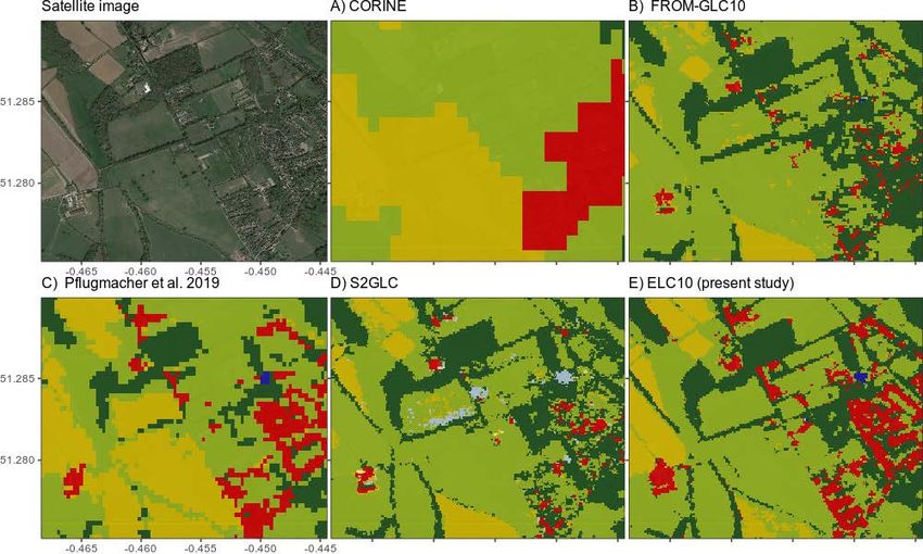
      Figure 9. Example of land cover classifications at the local scale for a selected landscape in Woking (south of London,
      England). Maps are shown for the present study relative to the four comparative datasets. Please refer to Supplementary
      Figures S3–S5 for more comparative examples.

                                 4. Discussion
                                 4.1. Comparison to State of the Art
                                       The ELC10 map produced here has accuracy levels (90.2%) that are comparable with
                                 multiple city- and country-scale Sentinel-based land cover maps globally [16]. Within
                                 the European context, we find that ECL10 has 18% less error than the CORINE dataset
                                 which is widely used for research and accounting purposes. This corroborates results from
                                 others [15,52] who have also found uncertainty and bias associated with CORINE maps.
                                 The primary explanation for this discrepancy in accuracy is that the CORINE minimum
                                 mapping unit (25 ha) is very coarse compared to Landsat- and Sentinel-based maps (e.g.,
                                 ELC10 minimum mapping unit of 0.01 ha). The CORINE project also adopts a bottom-up
                                 approach of consolidating nationally produced land cover datasets into one and is therefore
                                 prone to inconsistencies and spatial variations in mapping error. Although CORINE has
                                 been effectively used to stratify the probabilistic sampling of land cover for unbiased area
                                 estimates [53], it may not be functional in small municipalities or for other land use and
                                 ecosystem models that require fine-grained spatial data.
                                       To address the need for fine-grained land cover data, the European Space Agency
                                 recently initiated the development of the S2GLC map over Europe at 10 m resolution
                                 (http://s2glc.cbk.waw.pl/) [14]. The ELC10 map produced here extends on the S2GLC
                                 work by improving the overall accuracy by 7% and adopting an open source and trans-
                                 parent approach in a similar vein to the Landsat-based map by Pflugmacher et al. [15].
                                 Unlike previous pan-European maps, our approach relies on purely satellite-based input
                                 data and is therefore annually updatable for the foreseeable future lifespan of Sentinel and
                                 VIIRS sensors (assuming accuracy levels from LUCAS 2018 survey). It is thus indepen-
                                 dent of national topographic mapping datasets that take considerable resources to update
                                 (e.g., national land resource map of Norway; [54]. ELC10 also leverages Google’s cloud
                                 computing infrastructure, made freely available for research purposes through Google
                                 Earth Engine. We were able to train and make inference with our random forest model
                                 over 700 TB of satellite data at a rate of 100,000 km2 per hour which equates to approx.
                                 4 days of computing time to generate the 10 m product for Europe. In this way, regional
Remote Sens. 2021, 13, 2301                                                                                            16 of 22

                              or continental scale mapping of land cover, which has typically been the domain of large
                              transnational institutions, may become more democratised and independent of political
                              agenda [55].

                              4.2. Potential Applications
                                   As satellite technology and cloud computing improve, the ability to map land cover
                              at high spatial resolutions is becoming increasingly possible. This opens up a range of
                              novel use-cases for land cover maps at continental scales. One example is for mapping
                              small patches of green space within and outside of urban areas. Rioux et al. [56] found that
                              urban green space cover and associated ecosystem services were generally underestimated
                              at spatial resolutions coarser than 10 m. Similarly, green spaces constituting important
                              habitat for biodiversity such as semi-natural grasslands are often not portrayed in current
                              land cover maps. This is significant given that habitat loss is one of the main threats facing
                              biodiversity, particularly pollinator species, in agricultural landscapes across Europe [57,58].
                              Quantifying and monitoring the remaining fragmented habitat is therefore a conservation
                              concern at both regional and national levels [59]. This is also true for monitoring the
                              corollary of habitat loss–habitat restoration initiatives. Agri-environmental schemes [60]
                              such as the establishment of stone walls, hedge rows, and strips of semi-natural vegetation
                              along field margins are not detected by current land cover mapping initiatives. High-
                              resolution land cover maps such as the ELC10, presented here, provide a means to monitor
                              the status and trends of the remaining patches of semi-natural habitats and other small
                              green spaces over Europe. It is also possible to extend this mapping workflow to areas
                              outside of the European continent assuming there are reference data to calibrate the RF
                              model. This Google Earth Engine workflow may be particularly beneficial in monitoring
                              tropical ecosystems such as mangrove forests [61].

                              4.3. Limitations and Opportunities
                                     As with all land cover products, there are several limitations to ELC10 that are impor-
                              tant to note in the interest of data users and future iterations of pan-European land cover
                              maps. Our model produced classification errors that were greatest (accuracies below 80%)
                              in southern Europe due to the predominance of, and spectral similarity between shrubland
                              and bare land classes. For future refinements of the map one could aim to partition the LU-
                              CAS shrubland class into, e.g., 2–3 levels of vegetational succession. Although some regions
                              (i.e., central Europe, Figure 5) and classes (i.e., woodland: 95%, Table 2) exhibited much
                              higher accuracies than southern Europe, the error rate may still be significant, particularly
                              in the context of monitoring land use changes. A 95% accuracy implies that a land cover
                              class would have to change by 10% within a spatial unit (e.g., country or municipality)
                              from year to year in order for a map like ELC10 to detect it with statistical confidence.
                                     A major source of error in land cover models is the reference data. The LUCAS dataset
                              is vulnerable to geolocation errors due to GPS malfunctioning in the field, interpretation
                              errors and land cover ambiguities. For instance, the European Environment Agency
                              found that a post-screening of the LUCAS dataset increased CORINE-2000 accuracy by
                              6.4 percentage points [62]. In addition to mislabelled LUCAS points, intersecting Sentinel
                              pixels may contain mixed land cover classes and therefore introduce noise into the spectral
                              signal [25]. This is why the LUCAS Copernicus Module was initiated to produce quality-
                              assured homogeneous polygons for integration with earth observation. However, here we
                              found that intersecting Sentinel pixels with LUCAS polygon centroids did not significantly
                              improve classification accuracy relative to the raw theoretical LUCAS point locations alone
                              (Figure 3E). This finding supports the well-established characteristic of random forest
                              models which makes them robust against noisy training data [63]. It remains to be seen
                              whether utilising all pixels within LUCAS polygons increases accuracy further.
                                     Users of ELC10 should also be aware that our classification model is extrapolating into
                              areas without any reference data in countries including Norway, Switzerland, Liechtenstein,
                              and the non-EU Balkan states. However, because the LUCAS data cover a broad range of
Remote Sens. 2021, 13, 2301                                                                                           17 of 22

                              environmental conditions, it is reasonable to assume similar accuracies for neighbouring
                              countries, although this needs to be tested. The efficacy of integrating ground reference
                              samples with remote sensing may be illustrative for Norway and other countries and
                              stimulate future open-access land cover surveys. The fact that we found accuracies >85%
                              with
Remote Sens. 2021, 13, 2301                                                                                          18 of 22

                                   sive and therefore excludes its benefit of fast and on-the-fly land cover classifications
                                   where desirable. However, we acknowledge that we only used a single median and
                                   standard deviation per band and orbit mode for a full year of data. Speckle filtering
                                   may be more effective if one derives seasonal or monthly composites as inputs into
                                   the classifier, as we did with Sentinel-2 NDVI.
                              •    The fusion of Sentinel-1 and Sentinel-2 data has large increases in classification accu-
                                   racy (3–10%) and is therefore encouraged. The addition of auxiliary variables that
                                   capture large-scale environmental gradients important for distinguishing spectrally
                                   similar classes (e.g., shrubland and forest) also improve classification accuracies and
                                   should be included. However, users should be cautious of spatial overfitting to these
                                   auxiliary variables which may cause geographical biases due to spatial autocorrela-
                                   tions [72,73].
                              •    Cleaning reference samples through initiatives like the LUCAS Copernicus Module
                                   may not be worth the marginal gains in classification accuracy. RF models are robust
                                   against noisy training data [63] and therefore, so long as a clean validation sample
                                   is maintained, filtering noise in training data may not be necessary. Nevertheless,
                                   clean reference data supplied by the Copernicus Module is invaluable to deriving
                                   realistic accuracy estimates. We supplemented the Copernicus Module polygons with
                                   LUCAS points (n = 18,009) in order to balance class representativity in the training
                                   sample. We did this using an outlier removal procedure which may have artificially
                                   inflated our final accuracy estimates. Therefore, we recommend that initiatives like
                                   the Copernicus Module ensure that their sample is representative of the class area
                                   proportions in the study area, so that augmenting the training sample is not necessary
                                   for earth observation applications in the future.
                              •    Collecting tens of thousands of reference data points may also not be necessary de-
                                   pending on the desired classification accuracy. We found that accuracies above 85%
                                   are achievable with less than 5000 LUCAS points, albeit for an eight-class classifica-
                                   tion typology.
                              •    Cloud computing infrastructure like Google Earth Engine make ideal platforms given
                                   that we could produce a pan-European map within approx. 4 days of computation
                                   time from a single research user account.

                              5. Conclusions
                                    The recent proliferation of freely available satellite data in combination with advances
                              in machine learning and cloud computing has heralded a new age for land cover clas-
                              sification. What has previously been the domain of transnational institutions, such as
                              the European Space Agency, is now open to individual researchers and members of the
                              public. We present ELC10 as an open source and reproducible land cover classification
                              workflow that adheres to open science principles and democratises large scale land cover
                              monitoring. We find that combining Sentinel-2 and Sentinel-1 data is more important for
                              classification accuracy than the atmospheric correction and speckle filtering pre-processing
                              steps individually. We also confirm the findings of others that the random forest is robust
                              against noisy training data, and that investing resources in collecting tens of thousands
                              of ground-truth points may not be worth the gains in accuracy. Despite the effects of
                              data pre-processing, ELC10 has unique potential for quantifying and monitoring detailed
                              landscape elements important to climate mitigation and biodiversity conservation such as
                              urban green infrastructure and semi-natural grasslands. Looking to the future, maps like
                              ELC10 can be annually updated, and repeated in situ surveys like LUCAS can be used for
                              quantifying uncertainty and accuracy in area change estimates. Quantifying uncertainty
                              is crucial for earth observation products to be taken seriously by policy makers and land
                              use planners.
You can also read