Agricultural and Forest Meteorology
←
→
Page content transcription
If your browser does not render page correctly, please read the page content below
Agricultural and Forest Meteorology 296 (2021) 108216
Contents lists available at ScienceDirect
Agricultural and Forest Meteorology
journal homepage: www.elsevier.com/locate/agrformet
Biases in open-path carbon dioxide flux measurements: Roles of instrument
surface heat exchange and analyzer temperature sensitivity
M Julian Deventer a, b, *, Tyler Roman c, Ivan Bogoev d, Randall K. Kolka c, Matt Erickson a,
Xuhui Lee e, John M. Baker a, f, Dylan B. Millet a, Timothy J. Griffis a
a
University of Minnesota – Dept. Soil, Water & Climate, St. Paul, MN, USA
b
ANECO Institut für Umweltschutz GmbH & Co, Hamburg, Germany
c
US Forest Service – Northern Research Station Grand Rapids, Grand Rapids, MN, USA
d
Campbell Scientific, Logan, UT, USA
e
School of Forestry & Environmental Studies, Yale, New Haven, CT, USA
f
US Department of Agriculture (ARS) – Soil and Water Management Research, St. Paul, MN, USA
A B S T R A C T
Eddy covariance (EC) measurements of ecosystem-atmosphere carbon dioxide (CO2) exchange provide the most direct assessment of the terrestrial carbon cycle.
Measurement biases for open-path (OP) CO2 concentration and flux measurements have been reported for over 30 years, but their origin and appropriate correction
approach remain unresolved. Here, we quantify the impacts of OP biases on carbon and radiative forcing budgets for a sub-boreal wetland. Comparison with a
reference closed-path (CP) system indicates that a systematic OP flux bias (0.54 μmol m− 2 s− 1 ) persists for all seasons leading to a 110% overestimate of the
ecosystem CO2 sink (cumulative error of 78 gC m− 2). Two potential OP bias sources are considered: Sensor-path heat exchange (SPHE) and analyzer temperature
sensitivity. We examined potential OP correction approaches including: i) Fast temperature measurements within the measurement path and sensor surfaces; ii)
Previously published parameterizations; and iii) Optimization algorithms. The measurements revealed year-round average temperature and heat flux gradients of 2.9
◦
C and 16 W m− 2 between the bottom sensor surfaces and atmosphere, indicating SPHE-induced OP bias. However, measured SPHE correlated poorly with the
observed differences between OP and CP CO2 fluxes. While previously proposed nominally universal corrections for SPHE reduced the cumulative OP bias, they led to
either systematic under-correction (by 38.1 gC m− 2) or to systematic over-correction (by 17-37 gC m− 2). The resulting budget errors exceeded CP random uncertainty
and change the sign of the overall carbon and radiative forcing budgets. Analysis of OP calibration residuals as a function of temperature revealed a sensitivity of
5 μmol m− 3 K− 1 . This temperature sensitivity causes CO2 calibration errors proportional to sample air fluctuations that can offset the observed growing season flux
bias by 50%. Consequently, we call for a new OP correction framework that characterizes SPHE- and temperature-induced CO2 measurement errors.
1. Introduction et al., 2016).
Necessary for this endeavor are fast-response and accurate in
Networks of continuous trace gas flux measurements provide the struments that can resolve atmospheric scalar fluctuations near their
most direct tool for quantifying global biogeochemical cycles of green background levels across a wide range of hydro-meteorological condi
house gases (GHGs), and are critical for monitoring ecosystem responses tions. Accurate measurements of CO2 fluxes are of particular interest
to climate variations. The current generation of fast-response gas ana given their importance for climate change and because they form the
lyzers is able to directly resolve temporal and spatial variations in net foundation for understanding the carbon balance of ecosystems. EC-
ecosystem exchange (NEE) of the 4 most abundant greenhouse gases based CO2 flux measurements date back to the early 1970s (e.g. Des
(GHGs)—water vapor (H2O), carbon dioxide (CO2), methane (CH4), and jardins, 1974), but did not gain global popularity until the commercial
nitrous oxide (N2O)—by eddy covariance (EC) (Nemitz et al., 2018; development of fast response sonic anemometers and low-power open-
Rebmann et al., 2018). Globally synthesized long-term measurements of path (OP) infrared gas analyzers (e.g. Jones et al., 1967; Bingham et al.,
these GHG fluxes help constrain terrestrial carbon and nitrogen cycling 1978; Heikinheimo et al., 1989).
and the radiative forcing contributions of different ecosystems across the Despite over four intervening decades of measurements, technolog
globe. Such measurements are key to understanding the variability and ical and methodological refinements, debates about measurement arti
trajectory of the climate system (e.g. Petrescu et al., 2015; Baldocchi facts for OP gas analyzers persist. In particular, there are now many
* Corresponding author.
E-mail address: deventer@umn.edu (M.J. Deventer).
https://doi.org/10.1016/j.agrformet.2020.108216
Received 9 April 2020; Received in revised form 4 August 2020; Accepted 11 October 2020
0168-1923/© 2020 Elsevier B.V. All rights reserved.
M.J. Deventer et al. Agricultural and Forest Meteorology 296 (2021) 108216
reports of physiologically unreasonable OP-derived net CO2 uptake problematic given the extensive use of OP-derived flux data within the
fluxes during photosynthetically inactive periods and in ecosystems community. Based on a review of site documentation for the BASE data
lacking photosynthetically active vegetation (e.g. Hirata et al., 2005; products (AMERIFLUX 2019), early-generation LI-7500 instruments
Amiro, 2010; Welp et al., 2007; Wohlfahrt et al., 2008; Ono et al., 2008; have been deployed at more than 50 flux towers across the U.S. and
Lafleur and Humphreys, 2008; Ma et al., 2014; Wang et al., 2016; Hel Canada, yielding >300 site-years and >30,000 unique downloads of
big et al., 2016). Other studies have reported systematic discrepancies potentially biased flux data. This is a conservative estimate, as instru
between OP and concurrent closed-path (CP) EC or chamber measure mentation documentation is not provided publicly for a large number of
ments that persist into the growing season, manifesting as sites. Furthermore, Wang et al. (2017) report similar biases for
smaller-magnitude positive and larger-magnitude negative OP-derived later-generation OP sensors that consume lower power and are intended
fluxes (e.g. Anthoni et al., 2002; Ono et al., 2008; Järvi et al., 2009; to be bias-free.
Kittler et al., 2017; Holl et al., 2019). In a meta-study, Wang et al. (2017) Here we re-evaluate the currently-proposed corrections for SPHE-
found evidence of cold-season NEE open-path sensor artifacts across the induced flux biases at a cold sub-boreal wetland site via concurrent OP
majority of examined FLUXNET sites. Similar findings have been re and CP CO2 flux measurements. Specifically, we examine the un
ported in the marine flux community: for example, Butterworth and Else certainties and the systematic biases among the different correction
(2018) report that net CO2 uptake fluxes measured via OP EC over methods outlined above, and the implications for assessing ecosystem
land-fast sea ice were on average 25 times larger than chamber-derived carbon balance and radiative forcing based on eddy flux measurements
fluxes. Such discrepancies have now been reported for over 30 years (e. of CO2 and CH4.
g., Broecker et al., 1986).
The above findings have spurred an ongoing and unresolved debate 2. Methods
on the underlying mechanisms driving OP biases. Discussions evolved
around the Webb-Pearman-Leuning (WPL) formulations that account for 2.1. Measurement site and instrumentation
heat-, water vapor-, and static pressure-driven air density fluctuations,
which are required for OP flux calculations (Webb et al., 1980; Lee and Eddy covariance measurements were carried out at the Bog Lake
Massman 2011). Massman and Lee (2002) argued that in complex Peatland flux tower (US-MBP on AMERIFLUX) in the USDA Forest Ser
terrain (e.g. for tall canopies) and under high wind speeds, the WPL vice’s Marcell Experimental Forest (47.505 N, 93.489 W, Minnesota,
pressure variance term becomes significant, contradicting the common USA). The tower lies in an open natural peatland with short vegetation
practice of neglecting this effect. Under such conditions, erroneous sonic dominated by peat mosses (Sphagnum ssp). The climate is cold conti
temperature and consequently sensible heat flux measurements were nental with warm summers, characterized by mean annual precipitation
proposed to bias the OP flux calculations (Grelle and Lindroth, 1996). and temperature (1961-2009 reference period) of 780 mm and 3.4◦ C,
Subsequently, implausible OP fluxes were identified over simple terrain, respectively. The snow-covered period usually starts in November and
and under low wind speeds; such conditions render the above typically lasts for ~120 days. The site’s ecology, hydrology, and EC-
pressure-related mechanisms unlikely (Ono et al., 2008). Others have derived carbon balances have been described previously in Shurpali
postulated that thermal expansion and contraction of the instrument’s et al. (1993, 1995), Sebestyen et al. (2011), Olson et al. (2013), and
frame, contamination/degradation of optical components, instrument Deventer et al. (2019).
calibration drift, or incomplete surface energy balance closure could Three-dimensional wind velocity and sonic temperature measure
explain the observed OP flux artifacts (Serrano-Ortiz et al., 2008; Fratini ments were made using an ultrasonic anemometer (CSAT-3, Campbell
et al., 2014; Liu et al., 2006). Scientific Inc., Logan, Utah, USA) mounted 2.4 m above-canopy. An OP
Two proposed bias mechanisms have gained the most persistent CO2 and H2O infrared gas analyzer (LI-7500 from 04/2009-07/2015, LI-
attention in the EC community, specifically artifacts related to: 1) 7500A from 08/2015-present; LI-COR Biosciences Inc., Lincoln,
spectroscopic corrections; and 2) sensor path heat exchange (SPHE). Nebraska, USA) was positioned at the same height as the sonic
Edson et al. (2011), Kondo et al. (2014), Bogoev et al. (2015), Helbig anemometer (in reference to the center of its measurement path) and
et al. (2016), Wang et al. (2016), and Russel et al. (2019) showed that offset by 10 cm to the east. For a short period (2/15/2019 to 3/19/2019)
inaccurate/insufficient spectroscopic corrections (accounting for ab the LI-7500A was replaced by an identical sensor type of more recent
sorption line broadening due to barometric pressure, air temperature serial number. During this time the original LI7500A was refurbished
and dilution gases e.g. H2O) led to biased fluxes with two widely-used and factory-calibrated by LI-COR. The OP sensor was tilted by ~40
commercial non-dispersive infrared (NDIR) OP gas analyzers (EC150, degrees relative to the sonic anemometer to reduce retention of water
Campbell Scientific Inc., Logan, Utah, USA; LI-7500, LI-COR Bio droplets and particles on optical surfaces. The LI-7500A chopper hous
sciences, Lincoln, Nebraska, USA). In contrast, Burba et al. (2019) argue ing was maintained at 20◦ C year-round, matching the hard-coded fac
that aside from water vapor broadening, no spectroscopic corrections tory setup for the earlier-generation LI-7500. In this way the analyzer’s
are needed for the LI-7500 since the Boltzman distributions are heat emissions remained constant between both versions. Note that with
well-sampled, and thus temperature sensitivities are essentially elimi the introduction of the LI-7500A/RS updates, an optional “winter
nated. Steered by frequent reports of implausible LI-7500 flux mea setting” became available for this analyzer. In winter mode the power
surements under cold conditions, Grelle and Burba (2007) found consumption and heat production from the chopper motor housing are
evidence that heat exchange from OP sensor surfaces and from air within reduced to mitigate sensor-path heat exchange. This study did not
the measurement path is the dominant cause of OP measurement bias. evaluate the potential of the winter settings to minimize wintertime OP
An influential review on this mechanism (Burba et al., 2008) has biases.
informed the implementation of SPHE corrections in the widely-used Starting in November 2018, CO2 and H2O (dry) mole fractions were
“EddyPro” (LI-COR, Biosciences) open-source EC processing software. also measured with a CP analyzer (LI-7200, LI-COR Biosciences Inc.).
Since then, efforts have been initiated to revise previously-published Here, air was sampled through a 1 m insulated intake tube installed at
NEE budgets across regional flux networks to account for sensor sur the same height and offset 4 cm east from the sonic reference. The
face heating biases (e.g. Reverter et al. 2011). volumetric flow rate was maintained at ~14 l min− 1. Additionally, high-
Despite this broad implementation, only a few studies have experi frequency CH4 concentrations were measured with a low-power OP
mentally tested whether SPHE is the main driver of OP-derived flux analyzer (LI-7700, LI-COR Biosciences Inc.) that was vertically aligned
biases at their sites, and if the proposed corrections yield satisfactory but offset 40 cm south from the sonic reference. Methane-specific flux
constraints (Wohlfahrt et al., 2008; Järvi et al., 2009; Haslwanter et al., calculations and uncertainties were described earlier by Deventer et al.
2009; Kittler et al., 2017). This lack of systematic assessment is (2019).
2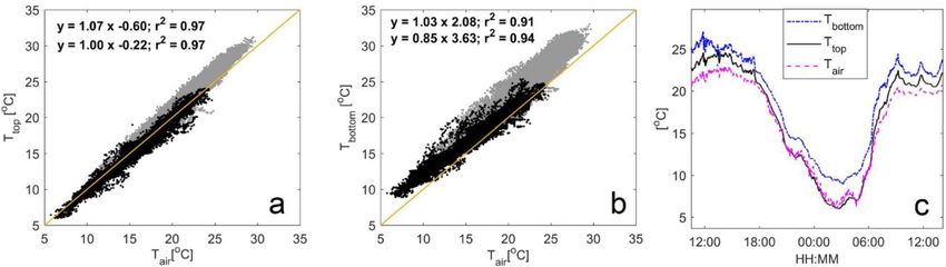
M.J. Deventer et al. Agricultural and Forest Meteorology 296 (2021) 108216
To monitor OP analyzer temperatures and calculate heat fluxes in the extra investment in measurements and data processing for direct SPHE
OP measurement path, fast ambient and sensor surface temperature measurements, to date there have been no independent studies evalu
measurements were made using fine-wire (FW) thermocouples (0.017 ating their potential for OP corrections. However, a few studies have
mm diameter; TT-T-40-SLE, OMEGA Engineering, Norwalk, CT, USA). evaluated the two nominally universal BC corrections (e.g. Järvi et al.,
These thermocouples were mounted in close proximity (≈1 cm) to the 2009; Helbig et al. 2016; Kittler et al., 2017).
LI-7500(A) bottom and top windows, and either directly fixed to the Within the BC framework, the sensible heat flux H in Eq. 1 is replaced
white instrument surfaces or at ~3 cm vertical distance from those by the measurement path sensible heat flux S (W m− 2), thereby taking
surfaces. To compare our FW measurements to the ones from Burba into account additional heat exchange from the instrument surfaces
et al., (2008) we average the two point-measurements to obtain an es (SOP ). If temperatures within the optical-path are measured, SPHE is
timate of LI-7500 optical path heat fluxes. Our method is different from calculated following:
the one deployed in Burba et al., (2008) who used platinum wire strung
(2)
′
across the entire measurement volume. Comprehensive auxiliary mea S = ρcp w′ TOP ,
surements are routinely performed at Bog Lake Peatland, with de
scriptions provided by Sebestyen et al. (2011) and Deventer et al. where TOP is the temperature measured within the LI-7500 optical-path.
(2019). If S is not measured directly, the BC method provides a
parameterization:
2.2. Traditional (WPL) open-path calculation: the default OP flux S = H + SOP , with SOP = Sbot + Stop + 0.15 Sspar . (3)
− 2
Here, SOP (W m ) is the instrument surface heat flux estimated from
We apply WPL theory to account for air density fluctuations in
the sum of heat fluxes from the bottom, top, and spars of the instrument
calculating OP-derived fluxes. For simplicity, we discuss only the carbon
(Grelle & Burba 2007; Burba et al., 2008). In controlled experiments, the
flux corrections here and formulate WPL in terms of the fluxes of water
authors observed a linear relationship between instrument surface
vapor and sensible heat. The resulting WPL-calculated flux (FOP ; kg m− 2
temperatures (Ts ) and ambient meteorological conditions, which was
s− 1) is hereafter designated the “default OP flux” (Webb et al., 1980):
then formulated either as a simple linear regression of Ts vs. Ta (referred
( )
ρ ρ ρ to here as the BC SLR approach) or as a multiple linear regression that
FOP = w’ ρc ’ + μ c E0 + c 1 + μ v H;
ρdry ρcp Ta ρdry (1) also includes radiation components and wind speed as independent
μ = 1.6077, variables (BC MLR approach):
TS,SLR = d1 Ta + d0 , (4)
where w is the vertical wind speed, ρc , ρv , ρdry , and ρ are the densities of
CO2, H2O, dry air, and air (kg m− 3), E0 is the H2O flux (kg m− 2 s− 1), cp is or
the specific heat of air (J kg− 1 K− 1), Ta is the air temperature (K), μ is the
air:water molecular mass ratio (unitless), and H is the ecosystem sensi TS,MLR = d1 Ta + d2 K + d3 U + d0 + Ta , (5)
ble heat flux (W m− 2). Overbars denote time averages and primes denote
where U is horizontal wind speed (m s− 1), and K is radiation flux (W
turbulent fluctuations.
m− 2), specifically incoming shortwave during day- and incoming long
wave radiation during nighttime. The SLR and MLR fitting coefficients
2.3. Open-path corrections accounting for sensor-path heat exchange
(d) are provided by Burba et al. (2008), and are differentiated by day- vs.
(SPHE)
night-time conditions. Surface temperatures are then passed to model
equations following Nobel (1983) that estimate instrument surface heat
Several correction approaches for SPHE have been proposed. In the
flux components based on the surface-to-ambient temperature gradient
following we present the theoretical framework for each approach that
scaled by laminar boundary layer thicknesses. The latter vary with
will later be evaluated against reference fluxes from the CP system.
horizontal wind speed and need to be modified by surface shape factors
(Burba et al., 2008). All empirical parameterizations and theoretical
2.3.1. Parameterizing instrument heat fluxes based on controlled
heat flux models within the BC framework were obtained assuming a
experiments: the “Burba” correction (BC)
vertical sensor placement, despite the manufacturer’s recommendation
Grelle and Burba (2007) found experimental evidence for SPHE that
of 10-15◦ sensor tilt to mitigate water or dust residue on the mirrors.
was greater than the actual ecosystem sensible heat fluxes (H), and that
originated from sensor surfaces that were either a few degrees warmer or
2.3.2. Direct path heat exchange parameterization: the “Wang” correction
cooler than ambient air. Three hypotheses were proposed to explain this:
Wang et al. (2017) derived a simplification of the BC approach that
(i) under cold conditions, electronic components can heat instrument
circumvents the underlying laminar boundary layer and surface tem
surfaces to above-ambient temperatures (sensor self-heating); (ii) on
perature model and directly estimates the instrument path heat flux S
clear days, solar radiation can heat exposed instrument surfaces to
from the ecosystem heat flux H. This is achieved by exploiting the linear
above-ambient temperatures (external heating); and (iii) on clear nights,
relationship between H and S reported by Burba et al. (2008):
radiative cooling can lead to below-ambient surface temperatures. Once
air density fluctuations due to internal and external SPHE had been ’
) H =bS− a,
’
( (6)
accounted for, Grelle and Burba (2007) and Burba et al. (2008) both with a’ = 2.67 W m− 2 , and b’ = 0.86.
reported good agreement between OP- and CP-derived CO2 fluxes.
Substituting into Eq. 1 yields the instrument heating-corrected flux:
Burba et al. (2008) introduced three different methods (hereafter
( ) [( ) ]
designated as Burba Corrections, “BC”) to account for the above effects; ρc ρ 1 a’
FWang = FOP + 1+μ v 1− ’ H− , (7)
these are distinct from the traditional WPL terms. The BC methods are ρcp Ta ρdry b b’
specific to the LI-7500 model and rely either on fast temperature mea
surements within the measurement path or are based on empirical which can be expressed as a linear regression on H :
models derived from controlled experiments. The first method is
FWang = FOP + b H + a, (8)
informed by direct heat flux measurements within the optical path of the
gas analyzer, and is thus recommended by Burba et al. (2008). The latter
with
two methods have the advantage that they can be applied (as universal)
to historic datasets, though without any direct validation. Owing to the
3
M.J. Deventer et al. Agricultural and Forest Meteorology 296 (2021) 108216
( )( ) [ 2]
ρc ρ 1 s complements the stepwise linear regression analysis by strengthening
b= 1+μ v 1 − ′ , in unit, 2 (9)
ρcp Ta ρdry b m our ability to identify the key explanatory variables and the likely
physical drivers of FOP − FCP .
and Our neural network construction follows standard community pro
( ) tocols (e.g. Moffat et al., 2007) and proceeds by splitting all available
ρc ρ data into training, optimizing and validation subsamples in a repeated
a= 1+μ v
ρc p T a ρdry randomized approach using k-means clustering. Details and uncertainty
( ) [ ] (10)
ρv ( a’ ) kg inference are as described in our past work (Deventer et al., 2019).
1+μ − ’
, in unit 2
.
ρdry b ms
2.4. Flux calculations and spectral corrections
Eq. 6 to Eq. 10 can be applied to historic datasets to obtain a CO2 flux
that is corrected for the effects of sensor surface heat exchange on the
Open- and closed-path fluxes were calculated, corrected, quality-
basis of co-measured sensible heat fluxes. The a and b coefficients
′ ′
controlled and filtered using the latest community protocols (Sabba
originate from Burba et al. (2008) based on a 1-week experiment in the
tini et al., 2018). Post-processing was performed in EddyPro 7.0 (LI-COR
non-growing season; it is an open question whether the same coefficients
Biosciences, Lincoln, USA). Closed-path H2O measurements were
can be reliably applied in other seasons and at other sites. This debate
aligned with vertical wind measurements using a relative
can only be resolved through direct measurements of S; it is not possible
humidity-dependent time lag optimization to compensate for H2O
to derive a parameterization based on H during the growing season
adsorption/desorption on inlet tubing surfaces. Spectral corrections for
when NEE and H are strongly related via ecophysiological and physical
high-frequency attenuation were calculated in two ways to assess the
processes.
associated uncertainty: 1) using an in-situ (empirical) method (Ibrom
et al., 2007; Fratini et al., 2012); and 2) using the analytical (theoretical)
2.3.3. Optimization via concurrent closed-path flux measurements: the
approach (Moncrieff et al. 1997). Attenuation due to sensor separation
“fitting” correction
(crosswind and vertical separation only) were corrected following Horst
An additional correction method that does not rely on temperature
and Lenschow (2009). Lastly, high-pass filtering effects due to
and heat flux models was discussed by Järvi et al. (2009) and slightly
de-trending were estimated following Moncrieff et al. (2005). For both
modified by Kittler et al. (2017). This correction applies a simplified
CO2 measurement systems the total spectral correction factors were
calculation of SOP and introduces a scaling coefficient to account for
similar, with median values of 1.11 (OP) and 1.13 (CP). The distribu
tilted sensor placement. Here, we re-evaluate their fitting method as:
tions of fluxes and of the OP - CP flux difference were insensitive to the
( )
(TS − Ta )ρc ρ choice of high frequency correction approach (p < 0.05, Wilcoxon
FFit = FOP + γ 1+μ v ,
ra (Ta + 273.15) ρdry (11) Rank-Sum Test). We therefore judge spectral correction uncertainties to
be negligible and use empirically-corrected fluxes for the sensor
with ra = Uu2* , inter-comparisons that follow.
where γ is a unitless coefficient interpreted as the fraction of Sop that is
being transported through the measurement cell, ra is the aerodynamic 2.5. Temperature sensitivities of the LI-7500 calibration function
resistance to heat transfer (s m− 1), ρc here in (µmol m− 3), and u* is the
friction velocity (m s− 1). Two parameterizations for TS have been used in In this work we also characterized the LI-7500 factory calibration
the past. The first one uses Eq. 4, whereas the second one follows a performance. Factory calibration follows the framework established by
polynomial: Welles and McDermitt (2005), with the OP analyzer measuring air
mixtures of variable and known CO2 concentrations under varying
TS = 0.0025 Ta2 + 0.9 Ta + 2.07. (12) ambient temperatures (− 25◦ C < Ta ≤ 43◦ C) in a climate chamber. A
5th-order polynomial is then derived fitting the measured absorptance
Here the γ and d parameters are estimated for night- and daytime
(α) to the corresponding gas concentrations. In our analysis we evaluate
conditions separately by non-linear least-squares optimization (initial
this approach by quantifying the calibration fit residuals (δρCO2 ) as a
guesses: γ = 0.05, d0 = 0, d1 = 1) (Järvi et al., 2009). We further
evaluate the performance of the fitting correction when γ is estimated function of ambient temperature at our site. Total infrared absorption in
using a fixed TS model (Eq. 12) following Kittler et al. (2017), and when the 4.26 micron CO2 absorption band depends not only on ρCO2 , but also
parameters are optimized to minimize bias (median absolute deviation, on the temperature of the air mixture due to the temperature depen
MAD) rather than sum of squares (SS). dence of the spectral line strength and the line shape (Gordon et al.,
2017). Thus, apparent changes in ρCO2 due to this δT δα
a
sensitivity can
2.3.4. Regression and machine learning based analysis of the potential falsely be interpreted as CO2 concentration changes; if correlated with
drivers of observed OP flux bias the vertical wind these will then manifest as flux errors. Such effects are
In addition to the existing corrections above, we apply machine fundamentally different from the WPL dilution effects and are termed
learning to the observed OP and CP flux differences using a variable spectroscopic effects associated with absorption line broadening.
combination of potential explanatory variables. A pre-selection of The LI-7500 internal calculation for CO2 number density is inde
explanatory variables was performed using stepwise linear regression pendent of ambient temperature (Eq. 3–19 and 3–23, LI-COR Bio
initiated with all variables used in the above SPHE corrections, i.e. Ta , U, sciences Inc 2015), corresponding to an assumption that calibration
incoming shortwave- and longwave radiation fluxes, the covariances errors do not correlate with ambient temperature fluctuations. The im
between w Ta and w ρv , and the means of ρc , ρv , and Ta . We then trained
′ ′ ′ ′ pacts of this assumption are reduced by maintaining the critical LI-7500
an ensemble of feed-forward artificial neural networks (ANNs) to predict optical components at constant temperature. In this study we investigate
the OP flux bias (i.e. FOP − FCP ). The most powerful set of explanatory the magnitude of the LI-7500 calibration error and how it corresponds to
variables was then determined based on statistical analysis against the observed flux errors relative to a closed-path system where
observed FOP − FCP data withheld from ANN training. The uniqueness of heat-exchange related measurement errors are substantially mitigated
this approach lies in the flexibility of neural networks to decipher non- because fluctuations in temperature are dampened by bringing the
linear relationships and interactions between explanatory variables sample air to a common temperature within the sample inlet and sample
without prior knowledge of functional dependencies. The approach cell. In the past, Bogoev et al. (2015) and Helbig et al. (2016) observed a
systematic bias in the IRGASON and the EC150 with a magnitude
4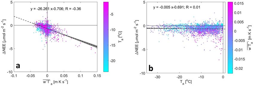
M.J. Deventer et al. Agricultural and Forest Meteorology 296 (2021) 108216
proportional to the sensible heat flux. They attributed the bias to the
temporally inadequate spectroscopic corrections of the thermistor probe
used in spectroscopic calculations.
3. Results
3.1. Plausibility of observed NEE
Between November 2018 and April 2019, the mean air temperatures
at Bog Lake Peatland was − 9◦ C, the mean soil temperatures at 10 cm
depth was 1.5◦ C, and the albedo exceeded 0.4. Weekly photographs
document a fully snow-covered vegetation canopy. Despite such
photosynthetically unfavorable meteorology and phenology, we
observed a strong correlation (r2 = 0.35) between OP-derived NEE and
H during this time, with a statistically significant (p < 0.05) and
negative slope. For the CP analyzer, however, the NEE-H correlation was
very weak (R2 = 0.01) with near-zero slope (Table 1). The positive
intercept in the CP NEE-H regression suggests ongoing microbial CO2
respiration in winter, even during nighttime, which can be explained by
above-zero soil temperatures (insulated from freezing air temperatures
by snow). The observed baseline respiration (0.3 µmol m− 2 s− 1) agrees Fig. 1. (a) Histograms of CO2 fluxes measured with open- (purple) and closed-
well with observations from flux chamber measurements made at path (black) analyzers from November 2018 through June 2019 (mean Ta =
SPRUCE (Hanson et al., 2016). − 3.7◦ C). Panels inset show median hourly fluxes (lines) with standard errors
In contrast, OP NEE-H regression results suggest net CO2 uptake at (shaded areas) for (b) November 2018 through April 2019 and (c) May 2019
near-zero values of H, and increasing net CO2 uptake during winter through June 2019.
daytime with increasing H. Based on the local meteorological and
phenological conditions we consider these fluxes to be physically un between day- and nighttime conditions. For the snow-covered season
realistic. Any systematic errors (excluding differences between OP vs. CP the default OP fluxes implied (on average) net CO2 uptake with a
measurement principles) inherent in the EC application or site-specific maximum around noon, whereas CP fluxes showed a relatively steady
violation of EC theory should be common to both the OP and CP release of CO2 throughout the day (Fig. 1b). During the growing season
fluxes as measurement height and sonic measurements were identical. the OP system measured larger net daytime CO2 uptake than did the CP
Observed OP - CP differences are thus assumed hereafter to reflect sensor, with the OP and CP CO2 fluxes tending to converge at night
biases in the OP measurements or in their associated flux calculations. In (Fig. 1c).
the following, we examine the magnitude of this bias, its persistence
throughout both cold and warm seasons, and its sensitivity to different
sensor-surface path heat exchange corrections. 3.3. Relation of NEE bias to environmental conditions
The largest Δ NEE episodes in this study were observed during pe
3.2. NEE bias
riods of largely positive ecosystem heat fluxes (p < 0.01, R2 = 0.12),
with larger negative OP biases associated with upward heat fluxes
The concurrent CO2 flux measurements reveal a persistent OP vs. CP
(Fig. 2a). This relationship was most evident in the snow covered season
NEE bias (Δ NEE = FOP − FCP ) (Fig. 1). Values of Δ NEE follow a double
(Δ NEE = − 26.3 w′ Ta − 0.71), but was also significant in the growing
′
exponential distribution skewed towards negative values; this OP ten
dency towards smaller-magnitude upward fluxes and/or larger- season (Δ NEE = − 4.1 w′ Ta − 0.31) as seen in Fig. 1c. In contrast, Δ NEE
′
magnitude downward fluxes manifested during the winter as well as values showed no significant relationship with horizontal wind speed (p
during the growing seasons (Fig 1b, c). The median Δ NEE value was = 0.11, R2 = 0.00) or with ambient temperatures on either weekly (p =
− 0.4 µmol m− 2 s− 1 with an inter-quartile range (IQR) of − 0.9 to − 0.1 0.65, R2 = − 0.03) or 30-min (p = 0.165, R2 = 0.00) timescales (Fig. 2b).
µmol m− 2 s− 1. When dividing Δ NEE by the CP flux it becomes apparent that the largest
The Δ NEE magnitude exhibited temporal variability at our site. In fractional biases occurred under near-zero ecosystem heat fluxes and
the growing season during daytime (albedo < 0.4; global radiation > 20 cold air temperatures (p < 0.01, R2 = 0.5).
W m− 2), the median fractional bias (ΔNEE |Fcp | ) was approximately 30% The negative Δ NEE:w’ Ta ’ intercept for all seasons (Fig. 2a) reveals
(− 0.36 µmol m− 2 s− 1). At night, biases were smaller (~14%, − 0.20 µmol the presence of a residual OP bias that is independent of ecosystem heat
m− 2 s− 1). During the snow-covered season, biases became much larger fluxes, suggesting increased SPHE due to OP sensor self-heating. How
(median ≈ 150%, − 0.46 µmol m− 2 s− 1) with less systematic difference ever, we find no significant differences in the ΔNEE : w′ Ta regression
′
coefficients under varying degrees of turbulence (all data, u* > 0.2, and
Table 1 u* > 0.35). Thus, while the OP measurement biases scale with heat
Orthogonal regression statistics between sensible heat fluxes and NEE. fluxes, they are independent of turbulence, suggesting that SPHE is not
Analyzer Coefficient 95% Confidence Limits the only reason for OP CO2 flux bias.
lower upper
In addition to the above single-variable regression analyses, we
− 2 − 1 − 2
performed multiple (stepwise) linear regressions (SLR) to test the degree
slope [(µmol m s )/(W m )]
to which a combination of explanatory variables could improve upon a
7200 − 0.003 − 0.005 − 0.001 model based on heat fluxes alone. We find that additional statistical
7500A − 0.023 − 0.024 − 0.022
power is provided by (in descending order of F statistics): w′ Ta , Ta , ρc ,
′
2 − 1
intercept [µmol m− s ]
ρv , w′ ρv ′ , and longwave radiation fluxes. Non-significant contributions (p
7200 0.324 0.307 0.342 > 0.05) were found for wind speed and shortwave radiation fluxes
7500A − 0.345 − 0.366 − 0.323
(Table 2). ANNs trained on combinations of the above variables confirm
5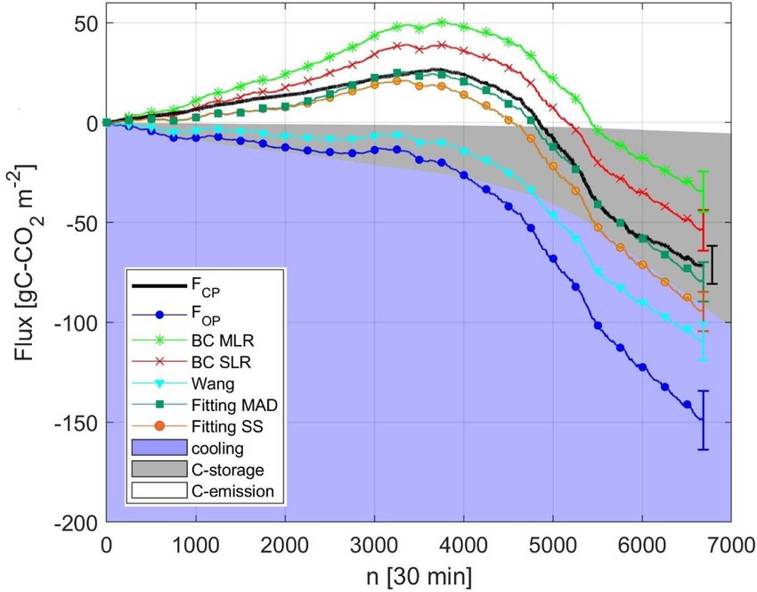
M.J. Deventer et al. Agricultural and Forest Meteorology 296 (2021) 108216
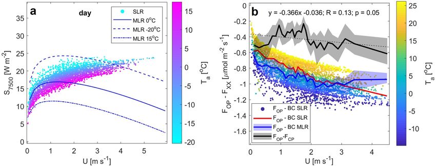
Fig. 2. Relationship between absolute flux bias (Δ NEE = FOP − FCP ), kinematic heat flux (w′ Ta ), and ambient temperatures (Ta ). Data plotted (n = 3061) are for the
′
snow-covered season (albedo > 0.4) when Ta < 0 ◦ C. Dashed lines and equations represent ordinary least squares regressions with 95% confidence intervals in
shaded gray.
Table 2
The relation between observed OP-CP flux differences and auxiliary variables. The top part of the table summarizes stepwise linear regression analyses. The bottom
panel summarizes the root mean square error and correlation coefficients between reference CP fluxes and OP fluxes after flux bias was predicted using artificial neural
networks (ANN) that were trained based on explanatory data combinations, that either excluded H2O terms*, or excluded temperature terms**.
Variable sum of squares sum of squares/df F p-value
w′ T a
′
255.3 255.3 243.8 5.40E-54
Ta 150.1 150.1 143.3 1.10E-32
ρc 68.1 68.1 65 8.80E-16
ρv 66.4 66.4 63.5 1.90E-15
w′ ρv ′ 25.5 25.5 24.3 8.30E-07
net longwave radiation 4.8 4.8 4.6 3.20E-02
Statistic FOP_ANN FOP_ANN (w/o H2O) FOP_ANN (w/o temperature) FOP
RMSD (FOP_ANN, FCP) 0.88 0.90 1.04 1.10
R (FOP_ANN, FCP) 0.93 0.92 0.90 0.89
R (Δ (FOP_ANN-FCP), Δ (FOP-FCP)) 0.50 0.47 0.31 n/a
*
w′ ρv ′ and ρv
**
w′ Ta and Ta
′
the overpowering importance of temperature terms (in particular the a much larger-than-predicted enhancement during daytime. Overall, the
kinematic heat flux) in explaining the observed Δ NEE (Table 2). The Ts vs. Ta regression parameters estimated here diverge from those of
SLR and ANN analyses both show that the inclusion of water vapor terms Burba et al. (2008) (Table 3), suggesting that these coefficients are
adds explanatory power to the models/networks (p < 0.05). This points site-specific (e.g. our OP tilt angle was ~40◦ vs. near-vertical alignment
towards previously identified CO2 measurement biases associated with in Burba et al. (2008)), rather than constants that can be applied
line broadening effects and direct absorption interference from water universally.
vapor (Welles and McDermitt 2005; Kondo et al., 2014). It thus appears Burba et al. (2008) noted that instrument surface temperatures are
that, in addition to SPHE, OP NEE biases may arise from incomplete likely to vary between sites due to tower- and sensor-placement specific
spectroscopic corrections. influences from shading, sun angle, and wind distributions. The aero
Overall, we find only weak evidence for the Δ NEE dependence on dynamic resistance to heat transfer decays approximately exponentially
environmental conditions proposed by Burba et al. (2008), indicating with wind speed. Thus, at low wind speeds surface temperatures can
that SPHE theory alone is insufficient to explain OP measurement bias. increase due to suppressed heat exchange and air parcel transport. In
In the following, we quantify the OP instrument surface temperatures Table 3 and below we examine uncertainties in the surface temperature
and analyzer path heat fluxes and assess the degree to which they model; these will later be propagated into the SLR correction to estimate
co-vary with ambient temperatures and ecosystem heat fluxes. its sensitivity to the parameter estimates from Table 3.
3.4. The extent and variability of OP surface heating 3.5. Relationship between sensor path heat exchange and ecosystem heat
fluxes
Instrument surface temperature measurements allow us to quantify
OP surface heating and assess the representativeness of the temperature Fig. 4 shows that heat fluxes measured close to the OP measurement
models presented in Burba et al. (2008). Our bottom-surface tempera path (S) differ from the true ecosystem heat fluxes (H), especially under
ture observations follow the trends observed in Burba et al. (2008), weakly established turbulence. In particular, S measured near the bot
namely: (i) surface temperatures varied near-linearly with ambient tom exceeded ambient heat fluxes measured by the sonic anemometer
temperatures; (ii) bottom-surface temperatures nearly always exceeded (H = 0.84 S + 13 W m− 2), with a mean bias error of 16.1 W m− 2. For
ambient temperatures during both day and night; and (iii) this offset was comparison, Burba et al. (2008) reported a similar slope (0.86), but a
enhanced at night and at low temperatures (Fig. 3). The top-surface smaller intercept (2.67 W m− 2) for their measurements over a clear-cut
temperatures agreed well with the Burba model at night but exhibited forest. We find here that the S -H differences become smaller (minimum
6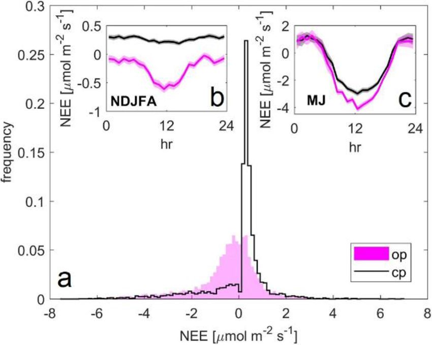
M.J. Deventer et al. Agricultural and Forest Meteorology 296 (2021) 108216
Fig. 3. Scatterplot (n > 30,000) of ambient vs. LI-7500A surface temperatures. Surface temperatures were measured in close proximity to the top (panel a) and
bottom (panel b) windows; data shown are separated into nighttime (black dots) and daytime (gray dots) with the 1:1 relation in yellow. Panel c shows an example
24-hour period (noon to noon, June 20th/21st 2019) with a large ambient temperature amplitude during mostly clear-sky conditions. Lines denote temperature
measurements near the bottom window (blue dash dotted), the top mirror (black solid) and in ambient air (magenta dashed).
in summer (as compared to H) (Table 4). When averaging our two S
Table 3 measurements to estimate OP representative S, we find a weak rela
Coefficients from regression analysis of ambient vs. sensor surface
tionship with Ta (R2 = 0.002; RMSD = 19.1 W m− 2; p < 0.01). Stepwise
temperaturesa.
linear regression yields best predictions using a 2-term model using
top bottom shortwave incoming radiation and U but yields negligible improvement
slope ( C/
◦
Intercept ( C)
◦
slope ( C/
◦
intercept (◦ C) in predictive power (R2 = 0.09; RMSD = 17.9 W m− 2; p < 0.01) over the
C) C) simple linear regression above, suggesting that seasonality in S-H is
◦ ◦
Daytime complex, complicating a robust parameterization of S(H).
This study 1.07 [1.06; − 0.60 [− 0.69; 1.03 [1.00; 2.08 [2.05; If the observed NEE bias is caused by OP surface heat exchange, we
1.11] − 0.58] 1.06] 2.23] expect to find a relationship between ΔNEE and S − H. Here we observe
Burba et al. 1.01 0.24 0.94 2.57
(2008)
only a very weak positive relationship between flux bias and S − H, both
Nighttime on an absolute (ΔNEE; p < 0.01, R2 = 0.01) and normalized
This study 1.00 [0.98; − 0.22 [− 0.23; 0.85 [0.83; 3.63 [3.60; (ΔNEE /|Fcp |; p < 0.01, R2 = 0.01) basis, suggesting that (within the
1.01] − 0.21] 0.88] 3.73] uncertainty of our S measurements) S − H does not in fact drive vari
Burba et al. 1.01 − 0.41 0.83 2.17
ability in ΔNEE. The sensor heating theory posits that the surface:
(2008)
ambient temperature gradient causes additional heat fluxes in the OP
a
values in brackets indicate the 95% confidence intervals. measurement path leading to air density fluctuations not accounted for
in the traditional WPL terms. Properly accounting for S should in that
of 9.0 W m− 2) and the S(H) regression becomes more linear with slopes case reduce the bias between OP and CP flux measurements. If, on the
close to unity for u* > 0.35 m s− 1 (Fig. 4c). During our study, S measured other hand, other sources of OP flux bias persist (e.g. inadequate spec
near the top yielded much smaller and on average negative (i.e. cooling) troscopic corrections) an SPHE-based dilution correction will be un
deviations from H, with a mean bias error of 1.1 W m− 2 and H = 1.36 S - successful in eliminating ΔNEE. In the following, we evaluate each of the
2 W m− 2. These results indicate that Sbot is partly offset by Stop . Seasonal SPHE corrections outlined in section 2.3 in terms of their performance in
analysis our S measurements as functions of H reveal that the heat reducing the ΔNEE observed in this study.
source from the bottom of the instrument is particularly large in winter,
and that the cooling from the top of the instrument is particularly large
Fig. 4. Panel a shows scatter plots of ecosystem heat fluxes (H) vs. heat fluxes measured close to the open-path windows (S) for the top surface (black) and bottom
surface (magenta) with orthogonal regression lines. Also shown (blue line) are the regression results of Burba et al. (2008) which represent path-averaged heat flux
measurements. Panel b shows the frequency distributions of the differences between OP and ecosystem heat fluxes measured. Panel c shows orthogonal regression
statistics for Sbottom vs. H binned into 0.05 m s− 1 friction velocity classes.
7
M.J. Deventer et al. Agricultural and Forest Meteorology 296 (2021) 108216
Table 4
Geometric regression estimates of SPHE as a function of ecosystem heat fluxes (H) with 95% confidence intervals in parenthesis. SPHE was measured near the top (Stop),
and near the bottom (Sbot) of the LI-7500A analyzer.
Sbot* Stop* mean(Sbot*,Stop*)
intercept slope intercept slope intercept slope
day snow 21.1 (20.2, 21.9) 1.65 (1.56, 1.75) 2.7 (2.3, 3.2) 0.94 (0.89, 1.0) 9.9 (9.4, 10.4) 1.07 (1.02, 1.13)
day green 19.3 (17.1, 21.5) 1.09 (1.04, 1.15) − 0.25 (− 1.5, 0.99) 0.73 (0.7, 0.75) 10.9 (9.3, 12.5) 0.89 (0.85, 0.93)
night snow 15.0 (14.3, 15.6) 1.19 (1.13, 1.25) 1.6 (1.3, 0.7) 0.70 (0.66, 0.71) 7.0 (6.6, 7.4) 0.83 (0.79, 0.87)
night green 16.0 (14.95, 16.97) 1.17 (1.05, 1.29) 1.0 (0.5, 1.4) 0.64 (0.58, 0.69) 8.0 (7.3, 8.7) 0.84 (0.76, 0.91)
*
here Sbot and Stop represent the measured heat flux in the LI-7500 path near the bottom or top mirror of the analyzer, and not just the heat emitted from the analyzer
surfaces alone.
CO2 m− 2—a bias of − 77.8 gC-CO2 m− 2, or 110% of the CP value. During
the snow-covered season, these two time series diverge with apparent
net CO2 uptake in the default FOP timeseries versus a steady increase in
the cumulative FCP values. Finally, although the CP- and default OP-
based cumulative NEE time series both decrease during the growing
season, the CO2 uptake rate inferred from the default OP dataset is
larger, thus further exacerbating the NEE bias accrued during the snow-
covered season. Cumulative flux differences between the default FOP and
reference FCP are much larger than the respective flux random errors
(Table 5).
Each of the SPHE corrections decreases the inferred OP sink strength
and hence the bias against the cumulative reference fluxes (Table 5).
Among them, the MLR and Wang methods respectively introduced the
largest (147%) and smallest (51%) corrections relative to the observed
FOP − FCP bias. Overall, the best agreement in terms of the cumulative
FOP − FCP flux difference was found for the Fitting method when opti
mized for MAD (− 8.4 gC-CO2 m− 2), and for the BC SLR method (17.4
gC-CO2 m− 2). Of all investigated correction approaches, only these two
yield cumulative fluxes within the uncertainty of the reference dataset
(Fig. 5, Table 5). Less accurate results were obtained from (in ascending
Fig. 5. Cumulative time series for default calculated (blue) and sensor-path
heat exchange (SPHE)-corrected open-path (OP) NEE estimates (BC SLR – red order of bias): the BC MLR method, the Fitting method when optimized
with crosses, BC MLR – green with asterisks, Wang – cyan with triangles, Fitting for SS, and the Wang method.
optimized for MAD – dark green with squares, Fitting optimized for SS – orange Table 5 and Fig. 5 show that one’s choice of OP correction approach
with circles). Also shown is the reference closed-path NEE estimate (thick black can change not only the magnitude but also the sign of the derived
line). Error bars denote the cumulative flux random errors in each case (Fin ecosystem C-balance and net radiative forcing. To illustrate this, we
kelstein and Sims, 2001). The error bar of the reference flux is offset to the right compare the range of OP NEE corrections to the wetland’s methane
for easier comparison. The graph background is color coded into C-emitting, budget derived via concurrent CH4 EC measurements. At the end of our
C-storing, and cooling regimes as discussed in-text. measurement period, the maximum discrepancy between cumulative
OP NEE estimates was ≈115 gC m− 2—greater than the threshold at
3.6. Cumulative fluxes which the ecosystem switches between net positive and negative radi
ative forcing (based on a 100 year forcing-neutral flux ratio of − 19.2
Quantification of OP biases is essential when deriving carbon and gC− CO2
(Petrescu et al., 2015)). Seasonally, the default OP fluxes,
gC− CH4
radiative forcing budgets used for global syntheses and model evalua
SPHE-corrected OP fluxes, and reference CP fluxes fall into 3 different
tions. As a first benchmark for the various OP corrections above, we
regimes: C-emitting, C-storing, and cooling, with the latter indicating
compare the cumulative NEE budget in each case with the correspond
net C storage sufficient to offset the radiative forcing of the wetland’s
ing reference CP NEE budget (Fig. 5, Table 5). While the CP measure
CH4 emissions. Such NEE uncertainties diminish our confidence in the
ments yield a cumulative (non-gap-filled, n = 6681) flux of − 71.3 gC-
radiative forcing budget of wetland sites; a better constraint on OP flux
CO2 m− 2, the default OP fluxes imply a much larger sink of − 149.1 gC-
Table 5
Carbon flux budgets from all deployed analyzers and all evaluated SPHE correction methods.
cumulative flux ± random error ΔFOP − FCP correction
correction relative to (FOP − FCP )
− 2 − 2 − 2
gC-CO2 m gC-CO2 m gC-CO2 m %
FCP − 71.3 ± 9.5
FOP − 149.1 ± 14.8 − 77.8
BC SLR − 53.9 ± 10.0 17.4 95.2 122
BC MLR − 34.5 ± 10.1 36.8 114.6 147
BC with measured S − 87.1 ± 9.5 − 15.8 62.0 83
Wang − 109.4 ± 9.5 − 38.1 39.7 51
Fitting MAD − 79.7 ± 9.8 − 8.4 69.4 89
Fitting SS − 94.62 ± 9.9 − 23.3 54.5 70
CH4 4.83 ± 0.9 gC-CH4
8
M.J. Deventer et al. Agricultural and Forest Meteorology 296 (2021) 108216
Table 6
Taylor diagram statistics of regression analysis between the reference NEE and the various corrected open-path flux estimates.
reference FCP default FOP BC MLR BC SLR Wang Fitting MAD Fitting SS
NEE mean (µmol m− 2 s− 1) − 0.49 − 1.03 − 0.24 − 0.37 − 0.76 − 0.55 − 0.65
NEE standard deviation (µmol m− 2 s− 1) 2.34 2.38 2.30 2.30 2.14 2.37 2.39
RMSE (µmol m− 2 s− 1) 1.10 1.08 1.10 1.08 1.20 1.08
correlation coefficient 0.89 0.89 0.89 0.89 0.88 0.89
bias error − 0.54 0.25 0.12 − 0.26 − 0.06 − 0.16
slope x = H *; y = NEE (µmol m− 2 s− 1/W m− 2) − 0.003 − 0.023 − 0.016 − 0.019 − 0.014 − 0.017 − 0.018
slope x = FCP ; y = FOP 1.13 0.98 0.98 1.02 0.98 0.98
*
orthogonal regression estimates for a period with Albedo > 0.4 and mean Ta = − 9 C; n = 3673
◦
biases is critical to better constrain these budgets. each temperature coefficient within its 95% confidence interval
(Table 3) and obtained minimum and maximum cumulative FOP cor
3.7. Correlation statistics of 30 min fluxes rections of 111 gC m− 2 and 131 gC m− 2, respectively. The resulting
( )
sensitivity index max−
mean
min
is ~17% (20 gC m− 2), or 25% of the bias
In addition to evaluating the OP correction approaches based on the
resulting cumulative fluxes, we examine here their correlation statistics between the default OP and reference CP fluxes (Table 5). This 17%
with respect to the reference CP fluxes on a 30-min timescale. Table 6 uncertainty arises solely from the 95% confidence interval of the SLR
shows that none of the evaluated corrections significantly improve the surface temperature model. Additional and likely larger uncertainties
correlation coefficients and RMSE over the default OP fluxes. All for the BC approach stem from radiation and wind speed parameter
investigated approaches yielded an FOP : FCP regression slope close to 1.0 uncertainties (in the case of MLR) and from assumptions of vertical heat
(± 0.03). As expected, the Fitting (optimized for MAD) method was most transfer through the measurement path (in the case of tilted sensors).
successful in minimizing bias errors, followed by the SLR method. The Burba et al. (2008) did not provide uncertainties for their boundary
Wang approach suppressed the flux standard deviation below that of the layer, temperature, or heat flux models, preventing any direct uncer
reference, and it most strongly reduced the spurious cold-season FOP : H tainty inference. However, from Fig. 2 and 3 in Burba et al. (2008) the
slope (section 3.1.). However, none of the corrected FOP : H slope esti scatter around their fitted temperature models is similar to that found
mates fall within a factor of 4 of the reference value. Based on this here, so that our error analysis above is likely a fair representation.
finding it is insufficient to constrain OP flux bias solely based on SPHE The SLR and MLR methods share identical surface boundary layer
theory. and surface heat flux formulations; differences between these correc
In the following we explore in detail the relevant error sources for tions thus arise solely from the instrument surface temperature param
each SPHE OP flux correction method. eterizations. We find here that: (i) for a given radiation flux SS,MLR and
SS,SLR diverge as a function of wind speed (Fig. 6a); (ii) in our study the
3.8. Evaluation of the Burba corrections SLR correction is systematically less than the MLR correction for wind
speeds < 3 m s− 1 and (iii) this relation is reversed at higher wind speeds
When considering historic OP datasets without available reference (Fig. 6b). Together, these observations explain the cumulative difference
flux measurements, a key question arises: How representative are the between MLR- and SLR-corrected fluxes found above (Fig. 5). We find
Burba et al. (2008) parameterizations for EC stations with variable that the cumulative SLR-corrected OP fluxes agree more closely with the
tower designs and sensor tilt? reference CP fluxes than do the MLR results (Fig. 5), with MLR corrected
To evaluate the sensitivity of the BC approach to the model tem OP fluxes higher (p < 0.05) than the SLR-corrected fluxes by 0.13 µmol
perature coefficients, we propagate the uncertainties associated with our m − 2 s− 1 .
measured surface and ambient temperatures (section 3.4) into the cu When applying the BC with directly measured S (Eq. 2) corrected
mulative flux time series. Specifically, we randomly resample (n = 1000) cumulative OP fluxes fall within the uncertainty of the reference fluxes
Fig. 6. Panel a shows calculated instrument surface heat fluxes (S7500 ) for the BC SLR method (dots, color mapped by air temperature) and for the BC MLR method
(lines). The latter were calculated for a radiation flux of 150 W m− 2 and for 3 different ambient temperatures. Panel b shows the differences between traditionally
calculated FOP to BC corrected fluxes as well as the difference to the closed-path (CP) reference flux as a function of wind speed. Lines show median values for n = 30
wind speed bins chosen to encompass equal number of flux differences. Shaded areas show the IQR of each bin. Dots show 30-min differences (FOP – BC SLR) heat-
mapped by ambient temperature. Also shown is the orthogonal regression (dashed black line) for the FOP - FCP relation with wind speed.
9
M.J. Deventer et al. Agricultural and Forest Meteorology 296 (2021) 108216
Table 7
Taylor diagram statistics of regression analysis between the reference NEE, default FOP and FOP corrected using BC with either directly measured S or modeled S. This
analysis was performed for a subset of the dataset, where S was directly measured near the top (Stop) and bottom (Sbot) of the OP analyzer (n = 2391).
reference FCP default FOP BC S from Sbot BC S from Stop BC S from mean(Sbot, Stop) BC S from SLR
− 2 − 1
NEE mean (µmol m s ) − 0.13 − 0.64 0.27 − 0.62 − 0.17 0.10
2 − 1
NEE standard deviation (µmol m− s ) 1.49 1.64 2.06 2.28 2.08 1.44
RMSE (µmol m− 2 s− 1) 0.00 0.78 1.46 1.33 1.24 0.83
correlation coefficient 1.00 0.88 0.70 0.83 0.81 0.83
bias error 0.00 − 0.51 0.40 − 0.49 − 0.05 0.13
2 − 1
slope x = H *; y = NEE (µmol m− s /W m− 2) − 0.004 − 0.020 − 0.031 − 0.045 − 0.025 − 0.045
slope x = FCP ; y = FOP 1.12 1.12 1.08 1.16 1.08
*
orthogonal regression estimates for a period with Albedo > 0.4 and mean Ta = − 9 C; ◦
(mean bias error = 0.05 µmol m− 2 s− 1). However, this cumulative example, FOP : FCP correlation coefficients remained unchanged at 0.89
agreement does not manifest in regression statistics of 30-min fluxes. We when minimizing the sum of squares. Kittler at al. (2017) likewise re
observe that OP fluxes corrected with BC using measured S yield worse ported minimal improvement in correlation coefficients (from 0.96 to
forecasting statistics against FCP as compared to the default FOP or FOP 0.97 during daytime, and from 0.81 to 0.82 during nighttime) when
corrected with BC SLR (Table 7). applying the same approach. When the Fitting corrections are performed
based on median absolute deviation (MAD), cumulative Δ NEE is
reduced from 23.3 to 8.4 gC-CO2 m− 2, i.e. to within the uncertainty of
3.9. Evaluation of the Wang correction
the reference flux (Table 5). The use of MAD optimization, however,
increases the RMSE above that of the default FOP (Table 6).
We next investigate the degree to which bias in OP-derived NEE
A cross-study comparison of γ estimates (Eq. 11; Table 8) suggests
estimates can be corrected solely on the basis of collocated sensible heat
that 6% to 18% (during daytime) and 4 to 9% (during nighttime) of heat
flux measurements. Applying Eq. 9 and 10 to our observations yields
from sensor surfaces is transported through the measurement path. A
coefficients (median with IQR) of a = − 0.17 (0.004) μmol m− 2 s− 1 and
larger degree of variability is observed for the temperature coefficient d
b = − 0.009 (0.001) (μmol m− 2 s− 1 )/(W m− 2 ). For comparison, Wang
(Table 8). Our γ and d estimates differ from those of Järvi et al. (2009),
et al. (2017) reported mean coefficients across 64 FLUXNET sites of a =
but are close to those of Kittler et al. (2017) who reported variability in γ
0.02 μmol m− 2 s− 1 and b = − 0.008 (μmol m− 2 s− 1 )/(W m− 2 ). as a function of wind speed and wind direction. We thus expect differing
When we estimate a and b directly from the observed relationship sensor orientation, tower design, and site climatology to cause vari
between H, S and FOP via directly measured instrument-path heat fluxes ability in γ and d between sites and studies.
(Eq. 2) rather than using Eq. 9 and Eq. 10 with default values for a and
′
We find here that the Fitting approach under-corrects the cumulative
b , the resulting coefficients are significantly larger: a = − 0.34 Δ NEE by 52.0, 28.1, and 24.7 gC-CO2 m− 2 when using coefficients from
′
μmol m− 2 s− 1 ; b = − 0.023 (μmol m− 2 s− 1 )/(W m− 2 ). These values fall at Järvi et al. (2009) (urban site), Järvi et al. (2009) (forest site), and
the upper end of the coefficients presented in the Wang et al. (2017) Kittler et al. (2017), respectively. All 3 corrections thus yield a larger
meta-analysis (which were not obtained from direct measurements). NEE bias than the universal BC SLR approach (17.4 gC-CO2 m− 2 over
This discrepancy between the calculated and parameterized a and b correction). Furthermore, the 3 Fitting corrections above yield respec
coefficients is due to the a and b constants in Eq. 7-10, which are from tive FOP : FCP RMSE values of 1.09, 1.15, and 1.08 µmol m− 2 s− 1, similar
′ ′
Burba et al. (2008) and not representative for our study site (section 3.4 or slightly worse than the result obtained for BC SLR (1.08 µmol m− 2
and 3.5). Direct estimation of a and b is thus recommended. s− 1).
3.10. Evaluation of the Fitting method 3.11. Temperature sensitivities of the LI-7500 calibration
We find that the Fitting approach does not appreciably improve the To quantitatively assess the temperature sensitivity of the LI-7500
linearity between the corrected OP and reference CP fluxes. For response we characterized its factory calibration performance under
Table 8
Optimization results for the parameters γ (fraction of heat transported through the sensor path, d1 (slope for the Ts : Ta regression), and d0 (intercept
for the Ts : Ta regression) used in Eqs. 10a and 10b, separated by day- and nighttime conditions.
γ d1 d0
(dimensionless) slope ( C/ C)
◦ ◦
intercept (◦ C)
Ts from Eq. 10a
this study day 0.180 ± 0.024 0.98 ± 0.002 1.43 ± 0.112
Järvi et al. (2009), urban day 0.060 ± 0.011 1.14 ± 0.010 1.77 ± 0.070
Järvi et al. (2009), forest day 0.085 ± 0.003 0.93 ± 0.010 3.17 ± 0.170
this study night 0.062 ± 0.008 0.89 ± 0.014 2.93 ± 0.129
Järvi et al. (2009), urban night 0.060 ± 0.011 1.13 ± 0.010 − 0.38 ± 0.040
Järvi et al. (2009), forest night 0.085 ± 0.003 1.05 ± 0.020 1.52 ± 0.140
Ts from Eq. 10b
this study day 0.098 ± 0.0024
Kittler et al. (2017) day 0.130 ± 0.0040
this study night 0.067 ± 0.0017
Kittler et al. (2017) night 0.042 ± 0.0030
Coefficients are shown ± 1 standard deviation from repeated optimizations based on 100 subsamples randomly drawn out of 75% of all data.
10You can also read