Climate of the past and present and its hydrological relevance - ITIA

School for Young Scientists:

 “Modelling and forecasting of river flows and managing
 hydrological risks: towards a new generation of methods”

 Moscow, Russia, 21-25 September, 2020

Climate of the past and present
and its hydrological relevance
 Demetris Koutsoyiannis
 Department of Water Resources and Environmental Engineering
 School of Civil Engineering, National Technical University of Athens
 (dk@ntua.gr, http://itia.ntua.gr/dk/)

 Available online: http://www.itia.ntua.gr/2065/

Parts of the presentation

1. Prologue: My personal involvement with climate
2. Weather and climate: Definitions, meaning and historical
 background
3. Climate of the past
4. Climate of the present
5. Basics of climate theory
6. The energy cycle
7. The carbon cycle
8. The hydrological cycle and its alleged intensification
9. The alleged intensification of hydrological extremes
10. Dealing with the future of climate and water
11. Epilogue: Is our future dark?
 D. Koutsoyiannis, Climate of the past and present 2

1. Prologue:
My personal involvement with climate

My first paper on climate
◼ This is my only journal paper with the term climate change in its
 title; it was rejected twice by Water Resources Research.
◼ It was accepted by Hydrological Sciences Journal, whose Editor,
 Zbigniew W. Kundzewicz, has been, at the same time, the IPCC
 leader for hydrology (Chairing Lead Author of the IPCC freshwater
 chapter in IPCC AR4 and Review Editor in IPCC AR5 & AR6).
◼ Later Kundzewicz, who appreciates diversity of opinion, invited me
 to jointly lead the Journal, which we did for more than a decade.
◼ The paper has now almost 400 citations.

 Koutsoyiannis (2003)

 Citations per year

Sources of images: https://scholar.google.com/citations?user=OPA_BScAAAAJ,
https://iahs.info/Publications-News/Hydrological-Sciences-Journal.do

 D. Koutsoyiannis, Climate of the past and present 4

My latest paper on climate (together with ZWK)
 Koutsoyiannis and Kundewicz (2020)

 D. Koutsoyiannis, Climate of the past and present 5

Dialogue and dialectic:
How science works (and Nature too)
◼ Tὸ ἀντίξουν συμφέρον καὶ ἐκ τῶν διαφερόντων
 καλλίστην ἁρμονίαν καὶ πάντα κατ' ἔριν
 γίνεσθαι.
 (Opposition unites, the finest harmony springs
 from difference, and all comes about by strife;
 Heraclitus, Fragment B 8).
◼ Γίνεσθαί τε πάντα κατ᾽ ἐναντιότητα καὶ ῥεῖν τὰ ὅλα ποταμοῦ
 δίκην, πεπεράνθαι τε τὸ πᾶν καὶ ἕνα εἶναι κόσμον […] καὶ τὴν
 μεταβολὴν ὁδὸν ἄνω κάτω, τόν τε κόσμον γίνεσθαι κατ᾽ αὐτήν.
 (All things come into being by conflict of opposites,
 and the sum of things flows like a river. Further, all
 that is limited and forms one world. […] Change [is]
 a pathway up and down, and this determines the
 evolution of the world; Heraclitus quoted by
 Diogenes Laertius IX.8).
 D. Koutsoyiannis, Climate of the past and present 6

Part 2
Weather and climate: Definitions,
meaning and historical background

The The Scientific School The Poetic School
importance Ἀρχὴ παιδεύσεως ἡ τῶν ὀνομάτων
 What’s in a name? That
 which we call a rose, by any
of ἐπίσκεψις (The beginning of other name would smell as
 education is the inspection of names) sweet.
definitions Socrates (from Epictetus, Discourses, Ι.17,12) William Shakespeare (“Romeo
 and Juliet”, Act 2, scene 2)
 Each definition is a piece of secret
 ripped from Nature by the human
 Let me argue that this
 spirit. I insist on this: any complicated
 situation [absence of a
 thing, being illumined by definitions,
 definition] ought not create
 being laid out in them, being broken
 concern and steal time
 up into pieces, will be separated Into
 from useful work. Entire
 pieces completely transparent even to
 fields of mathematics
 a child, excluding foggy and dark
 thrive for centuries with a
 parts that our intuition whispers to us
 clear but evolving self-
My own view: while acting, separating into logical
 image, and nothing
I am not a poet. pieces, then only can we move further,
 resembling a definition.
I strongly believe that towards new successes due to
 Benoit Mandelbrot (1999, p. 14)
in science we should definitions . . .
follow Luzin. Nikolai Luzin (from Graham and Kantor, 2009)
 D. Koutsoyiannis, Climate of the past and present 8

Weather – Tempus – Καιρός
◼ Weather is the state of the atmosphere at a
 particular time, as defined by the various
 meteorological elements (WMO, 1992)1.
◼ The elements are meteorological variables: e.g.,
 pressure, temperature, humidity, precipitation,
 cloudiness, visibility and wind.
◼ It is often used with respect to its effects upon life
 and human activities2.
◼ In Greek and Romance (Neo-Latin) languages the
 Source: https://lsj.gr/wiki/καιρός
 term has also the meaning of time.
◼ In English and Greek (not in all languages), weather
 Greek Καιρός
 refers to short-scale (min to d) variations in the
 atmosphere and is distinguished from climate. Italian Tempo
 French Temps, Météo
1 See also the glossary of the NOAA's National Weather Service: Spanish Tiempo, Clima
https://w1.weather.gov/glossary/index.php?letter=w. Portuguese Tempo, Clima
2 Cf. the glossary of the American Meteorological Society,
 Russian Погода
http://glossary.ametsoc.org/wiki/Weather
 D. Koutsoyiannis, Climate of the past and present 9

Climate < Clima < Κλίμα: Definitions1
 ◼ Climate system is the system consisting of the atmosphere,
 hydrosphere (including its solid phase, cryosphere),
 lithosphere and biosphere, which mutually
 interact and respond to external influences.
 ◼ Climatic processes are the physical, chemical and
 biological processes, which are produced by the
 interactions and responses of the climate system
 components through flows of energy and mass,
 and chemical and biological reactions.
 ◼ Climate is a collection of climatic processes
 at a specified area, stochastically characterized
 for a range of time scales.
 Source: https://en.wikipedia.org/wiki/Climate_system
 ◼ The term process means change (Kolmogorov,
 1931). Thus, climate is changing by definition.
 ◼ The term stochastic means random (i.e., unpredictable, unknowable in deterministic
 terms) and the term stochastic process means a family of stochastic (random) variables
 indexed by time .
 ◼ The terms stochastic characterization and stochastics collectively refer to the scientific
 areas of probability, statistics and stochastic processes.
 ◼ The term hydroclimatic is used to give more emphasis on the hydrological processes.
1 My definitions (Koutsoyiannis, 2021) are based on, but are not identical to, common ones in the
literature (see next slides).
 D. Koutsoyiannis, Climate of the past and present 10

Climate < Clima < Κλίμα: History
◼ Aristotle (384–322 BC) in his Meteorologica describes
 the climates on Earth in connection with latitude but
 he does not use the term climate. Instead, he uses
 the term crasis (κρᾶσις, literally meaning mixing,
 blending, temperament; cf. εὔκρατος, εὐκρασία).
◼ The term climate (κλίμα, plural κλίματα) was coined
 as a geographical term by the astronomer Hipparchus
 (190 –120 BC; founder of trigonometry). It originates
 from the verb κλίνειν, meaning ‘to incline’ and
 denoted the angle of inclination of the celestial
 sphere and the terrestrial latitude characterized by
 this angle.
◼ Hipparchus’s Table of Climates is described by Stabo
 the Geographer (63 BC – AD 24), from whom it
 becomes clear that the Climata of that Table are just
 latitudes of several cities, from 16° to 58°N (see
 Shcheglov, 2007, for a reconstruction of the Table).
◼ Furthermore Strabo, defined the five climatic zones,
 torrid (διακεκαυμένη), two temperate (εὔκρατοι) and
 two frigid (κατεψυγμέναι), as we use them to date. Source: https://lsj.gr/wiki/κλίμα

 D. Koutsoyiannis, Climate of the past and present 11

Climate < Clima < Κλίμα: Contemporary history
◼ The term climate was used with the ancient Greek geographical meaning
 until at least 1700. The term climatology appears after 1800.
◼ With the increasing collection of meteorological measurements, the term
 climate acquires a statistical character as the average weather. Indeed, the
 geographer A.J. Herbertson (1907) in his book entitled “Outlines of
 Physiography, an Introduction to the Study of the Earth”, gave the following
 definition of climate, based on weather (but also distinguishing it from
 weather):
 By climate we mean the average weather as ascertained by many years'
 observations. Climate also takes into account the extreme weather
 experienced during that period. Climate is what on an average we may
 expect, weather is what we actually get.
◼ Herbertson also defined climatic regions of the world based on statistics of
 temperature and rainfall distribution.
◼ Herbertson’s work was influential for the famous and most widely used
 Köppen (1918) climate classification; this includes six main zones and eleven
 climates which are on the same general scale as Herbertson's (Stamp, 1957).
 D. Koutsoyiannis, Climate of the past and present 12

Climate < Clima < Κλίμα: Some modern definitions
◼ Definition by the USA National Weather Service, Climate Prediction Center
 (https://www.cpc.ncep.noaa.gov/products/outreach/glossary.shtml#C):
 Climate – The average of weather over at least a 30-year period. Note that the climate taken
 over different periods of time (30 years, 1000 years) may be different. The old saying is climate
 is what we expect and weather is what we get.
◼ Definition by the American Meteorological Society (http://glossary.ametsoc.org/wiki/Climate):
 Climate – The slowly varying aspects of the atmosphere–hydrosphere–land surface system. It
 is typically characterized in terms of suitable averages of the climate system over periods of a
 month or more, taking into consideration the variability in time of these averaged quantities.
 Climatic classifications include the spatial variation of these time-averaged variables.
 Beginning with the view of local climate as little more than the annual course of long-term
 averages of surface temperature and precipitation, the concept of climate has broadened and
 evolved in recent decades in response to the increased understanding of the underlying
 processes that determine climate and its variability.
◼ Definition by the IPCC (2013)
 Climate – Climate in a narrow sense is usually defined as the average weather, or more
 rigorously, as the statistical description in terms of the mean and variability of relevant
 quantities over a period of time ranging from months to thousands or millions of years. The
 classical period for averaging these variables is 30 years, as defined by the World
 Meteorological Organization. The relevant quantities are most often surface variables such as
 temperature, precipitation and wind. Climate in a wider sense is the state, including a
 statistical description, of the climate system.
 D. Koutsoyiannis, Climate of the past and present 13

Some remarks on climate’s modern definitions
◼ Why “at least a 30-year period”? Is there anything special with the 30 years?
 ❑ This reflects a historical belief that 30 years are enough to smooth out “random”
 weather components and establish a constant mean. In turn, this reflects a perception
 of a constant climate—and a hope that 30 years would be enough for a climatic
 quantity to get stabilized to a constant value. It can be conjectured that the number 30
 stems from the central limit theorem and in particular the common (albeit wrong)
 belief that the sampling distribution of the mean is normal for sample sizes over 30
 (e.g. Hoffman, 2015). Such a perception roughly harmonizes with classical statistics of
 independent events.
 ❑ This perception is further reflected in the term anomaly (from the Greek ανωμαλία,
 meaning abnormality), commonly used in climatology to express the difference from
 the mean.
 ❑ Thus, the dominant idea is that a constant climate would be the norm and a deviation
 from the norm would be an abnormality, perhaps caused by an external agent.
 ❑ The entire line of thought is incorrect.
◼ Why “climate taken over different periods of time (30 years, 1000 years) [is] different”?
 ❑ The obvious reply is: Because different 30-year periods have different climates. This
 contradicts the tacit belief of constancy and harmonizes with the perception of an
 ever-changing climate.
◼ Is Herbertson’s idea, “climate is what we expect, weather is what we get”, correct?
 ❑ No. A correct reformulation would be “weather is what we get immediately, climate is
 what we get if we keep expecting for a long time” (Koutsoyiannis, 2011).
 D. Koutsoyiannis, Climate of the past and present 14

The meaning of “climate change”
 ◼ In scientific terms, the content of the term climate change is almost equivalent to
 that of weather change or even time change (climate is changing as is weather and
 time).
 ◼ Thus, “the term 'climate change' is a misleading popular slogan” (Vit Klemes†) and
 serves political aims. It is not a scientific term.
 ◼ Even according to the IPPC’s (2013) definition, its meaning is ambiguous:
 Climate change refers to a change in the state of the climate that can be identified
 (e.g., by using statistical tests) by changes in the mean and/or the variability of its
 properties, and that persists for an extended period, typically decades or longer.
 Climate change may be due to natural internal processes or external forcings such
 as modulations of the solar cycles, volcanic eruptions and persistent
 anthropogenic changes in the composition of the atmosphere or in land use.
 Note that the Framework Convention on Climate Change (UNFCCC), in its Article 1,
 defines climate change as: ‘a change of climate which is attributed directly or
 indirectly to human activity that alters the composition of the global atmosphere
 and which is in addition to natural climate variability observed over comparable
 time periods’. The UNFCCC thus makes a distinction between climate change
 attributable to human activities altering the atmospheric composition, and climate
 variability attributable to natural causes.
† 1932-2010; https://motls.blogspot.com/2011/03/vit-klemes-1932-2010.html

 D. Koutsoyiannis, Climate of the past and present 15

Evolution of the use of the term “climate change”
 Source: https://books.google.com/ngrams/graph?content=climate+change%2Cgood+day
 &case_insensitive=on&year_start=1900&year_end=2005&corpus=15&smoothing=0

 A neutral two-word everyday
 expression for comparison

◼ The graph shows the evolution of the frequency of appearance of the term “climate
 change” in the millions of books archived by Google Books. The neutral term “good
 day” is used as a reference for comparison.
◼ The term appeared in the 1970s.
◼ It looks that after 1990 climate change became more important than good day.

 D. Koutsoyiannis, Climate of the past and present 16

The launch of the Climate Change Agenda
 ◼ Henry Kissinger, the then powerful
 Secretary of State and National
 Security Advisor of USA raised the
 issue of “climatic changes” in the UN
 Assembly in 1974.
 ◼ WMO reacted immediately (in a
 month).
 Kissinger (1974)

 WMO (1974)

 Reproduced
 from
 Lewin (2017)

 D. Koutsoyiannis, Climate of the past and present 17

Scientists get involved immediately: NOAA, Oct. 1974
 ◼ Was the climate alert about
 global cooling or global warming?
 ◼ The answer was not categorical
 and in fact did not matter.
 ◼ What did matter was the alert
 per se.

Hughes (1974)

 D. Koutsoyiannis, A voyage in climate, hydrology and life 18

The first book with a
title containing
“climate change”

 CIA (1976)

A cold-war report referring to USSR, in
which climate change is the cooling of
the Northern Hemisphere since 1940.
 D. Koutsoyiannis, Climate of the past and present 19

A necessary clarification ending Part 2

◼ “Climate change” is a political agenda—not anything
 scientifically sound.
◼ What follows purports to be scientific—not political.
◼ I have also conducted research on the political, historical and
 socio-economic aspects of the Climate Change Agenda.
◼ Those in the audience interested in my latter research are
 invited to visit my presentation (Koutsoyiannis 2020b):

 The political origin of the Climate Change Agenda
 http://www.itia.ntua.gr/2035/

 D. Koutsoyiannis, Climate of the past and present 20

Part 3
Climate of the past

“Πάντα ρεῖ”1 & “Μεταβάλλει τῷ χρόνῳ πάντα”2
Changes on Earth since the appearance of earliest
life, 4 billion years ago
 1.8 10000
 The graph has been
 Earth rotation constructed from

 CO₂ concentrtation. ratio to present day value
 1.6 rate
 estimates by Kuhn et al.
(all variables except CO₂ concentrtation)

 1.4 Temperature, (1989). Temperature is
 1000 Kasting (1987) expressed in K and
 Ratio to present day value

 1.2
 Temperature, corresponds to 35°
 1 Hart (1978) latitude; a change in the
 100
 Solar constant temperature ratio by 0.01
 0.8
 (solar radiation) corresponds to ~2.9 K.
 0.6 Although the estimates
 Land area
 10 are dated and uncertain,
 0.4
 CO₂ concentr., evidence shows existence
 0.2
 Time’s
 Time's arrow
 arrow Kasting (1987) of liquid water on Earth
 0 1 CO₂ concentr.,
 even in the early period,
 4 3 2 1 0 Hart (1978) when the solar activity
 Billion years before present
 was smaller by 20-25%.
 ______ This is known as the faint
 1 “Everything flows” Heraclitus, quoted in Plato’s Cratylus, 339-340 young Sun problem
 2 “Everything changes in course of time”, Aristotle, Meteorologica, I.14, (Feulner, 2012).
 353a 16
 D. Koutsoyiannis, Climate of the past and present 22

Sea level during the Phanerozoic
 600
 Exxon sea level curve, Haq et al. (1987)
 500
 Exxon sea level curve, Haq and Al-Qahtani (2005)
 400
 Hallam (1984)
 300
Sea level (m)

 200
 100
 0
 Time’s
 Time'sarrow
 arrow
 -100
 600 550 500 450 400 350 300 250 200 150 100 50 0
 Million years before present
 Proterozoic Paleozoic Mesozoic Cenozoic

 Quaternary
 Ordovic- Silur- Carboni- Paleo- Neo-
 Ediacaran Cambrian Devonian Permian Triassic Jurassic Cretaceous
 ian ian ferous gene gene

 Phanerozoic = Paleozoic + Mesozoic + Cenozoic. High sea level suggests high temperature.
 Digitized data sources:
 For Haq et al. (1987): https://figshare.com/articles/Haq_sea_level_curve/1005016.
 For Haq and Al-Qahtani (2005):
 https://web.archive.org/web/20080720140054/http://hydro.geosc.psu.edu/Sed_html/exxon.sea;
 Note though that it has discrepancies from the graph in Miller et al. (2005).
 For Hallam (1984), data were digitized in this study using chronologies of geologic eras from the
 International Commission on Stratigraphy, https://stratigraphy.org/chart.
 For other reconstructions see van der Meer (2017).

 D. Koutsoyiannis, Climate of the past and present 23

Life evolution and sea level during the Phanerozoic

 Cretaceous–Paleogene extinction
 Complex multicellular organisms

 Ordovician–Silurian extinction

 Permian–Triassic extinction
 Sharks, insects, land plants

 Triassic–Jurassic extinction
 Late Devonian extinction

 Dinosaurs, fist mammals

 Homo sapiens
 Arachnids, scorpions

 First birds (toothed)
 Fish, vertebrates

 Flowering plants
 Animals on land

 Amphibians

 SARS-CoV-2
 Mammals
 Tetrapods

 Primates
 Conifers
 Reptiles

 Homo
 Bees
 600
 Exxon sea level curve, Haq et al. (1987)
 500 Exxon sea level curve, Haq and Al-Qahtani (2005)
 400 Hallam (1984)
 Creation events
 300
Sea level (m)

 Extinction events
 200
 100
 0
 Time’s
 Time'sarrow
 arrow
 -100
 600 550 500 450 400 350 300 250 200 150 100 50 0
 Million years before present
 Proterozoic Paleozoic Mesozoic Cenozoic

 Quaternary
 Ordovic- Silur- Carboni- Paleo- Neo-
 Ediacaran Cambrian Devonian Permian Triassic Jurassic Cretaceous
 ian ian ferous gene gene

 ◼ Q: When did extinction happen? On temperature rise or fall?
 D. Koutsoyiannis, Climate of the past and present 24

Co-evolution of temperature, CO₂ concentration and
sea level in the Phanerozoic
 40
 Scotese (2018)
 35
 Temperature T (°C)

 30
 25
 20
 15
 10
 600 550 500 450 400 350 300 250 200 150 100 50 0
 10000
 CO₂ conc. (ppmv)

 1000

 100
 Davis (2017) Berner (2008) Ekart et al. (1999)
 10
 600 600 550 500 450 400 350 300 250 200 150 100 50 0
 500
 Sea level (m)

 400
 300
 200
 100
 Hallam (1984)
 0 Time’s arrow
 -100
 600 550 500 450 400 350 300 250 200 150 100 50 0
 Million years before present
 Proterozoic Paleozoic Mesozoic Cenozoic

 Quaternary
 Ordovic- Silur- Carboni- Paleo- Neo-
 Ediacaran Cambrian Devonian Permian Triassic Jurassic Cretaceous
 ian ian ferous gene gene

 D. Koutsoyiannis, Climate of the past and present 25

Temperature change in different time windows
from observations and proxies Markonis and Koutsoyiannis (2013)
 1.5 6

 T (oC)
 CRU & NSSTC EPICA 4

 δT
 1
 2
 0.5
 0
 0 -2
 -0.5 -4
 -1 -6
 -1.5 -8
 -10
 -2
 -12
 1850 1870 1890 1910 1930 1950 1970 1990 2010
 Year 800 700 600 500 400 300 200 100 0
 Thousand Years BP
 1 -1.5

 δT
 Moberg & Lohle

 δ18Ο
 Huybers
 0.5 -1
 0 -0.5
 -0.5
 0
 -1
 0.5
 -1.5
 1
 0 200 400 600 800 1000 1200 1400 1600 1800
 Year
 2500 2000 1500 1000 500 0
 Thousand Years BP
 -35 0

 δ18Ο
 Taylor Dome

 δ18Ο
 -37 1

 -39 2

 -41 3

 -43 4
 Zachos
 -45 5
 10 9 8 7 6 5 4 3 2 1 0 50 45 40 35 30 25 20 15 10 5 0
 Thousand Years BP Million Years BP
 15
 -30
 Veizer

 δΤ
 GRIP -32
 δ18Ο

 10
 -34
 -36
 -38 5
 -40
 -42 0
 -44
 -46 -5
 -48
 -50 -10
 100 90 80 70 60 50 40 30 20 10 0 500 450 400 350 300 250 200 150 100 50 0
 Thousand Years BP Million Years BP

 D. Koutsoyiannis, Climate of the past and present 26

Focus on the last deglaciation: temperature
 -25
 Pleistocene
 Abrupt
 -30
 changes
 Temperature (°C)

 -35

 -40

 -45 Younger Dryas
 cool period

 -50 Holocene
 Glacial Transient Interglacial Experimental drilling on the
 -55 Greenland Ice Cap in 2005,
 -20000 -18000 -16000 -14000 -12000 -10000 -8000 -6000 -4000 -2000 0 2000 https://earthobservatory.nasa.
 gov/features/Paleoclimatology
 Calendar year ('+' = AD, '-' = BC) _IceCores
Noticeable facts:
(1) The difference of the interglacial from glacial temperature is > 20 °C.
(2) In periods of temperature increase, the maximum rate of change has been 8.5
°C/century.
(3) In periods of decrease, the maximum rate has been -4.3 °C/century.
Data: Temperature reconstruction from Greenland ice cores; averages from GISP2, NGRIP and NEEM Ice Drilling
locations as given by Buizert et al. (2018) for a 20-year time step (available from https://www.ncdc.noaa.gov/paleo-
search/study/23430).
 D. Koutsoyiannis, Climate of the past and present 27

Focus on the last deglaciation: sea level
22050 20050 18050 16050 14050 12050 10050 8050 6050 4040 2050 50 BC 1950 AD

 Max increase rate:
 15 m / 500 years =
 30 mm/year

Source: https://commons.wikimedia.org/wiki/File:Post-Glacial_Sea_Level.png
 D. Koutsoyiannis, Climate of the past and present 28

Focus on the last 10 thousand years: temperature
 -26 Medieval warm period:
 Minoan climate optimum: 1940, -27.8
 -1020, -27.0 700, -26.5
 -27 -5840, -26.7
Temperature (°C)

 -28

 -29
 Roman climate optimum:
 ±1, -27.4
 -30
 180, -30.4
 -31 840, -30.3
 -6240, -30.6 20-year time step
 500-year average 1860, -31.3
 -32
 -8000 -7000 -6000 -5000 -4000 -3000 -2000 -1000 0 1000 2000
 Calendar year ('+' = AD, '-' = BC)
 Noticeable facts:
 (1) 1940 was warmer than present. (2) The warmest period was around 700 AD. (3) There
 has been a dominant cooling trend for more than 7000 years.
 Data: Greenland ice cores as in a previous slide.
 D. Koutsoyiannis, Climate of the past and present 29

Part 4
Climate of the present

Recent global sea-level rise
 50
 Dangendorf et al. (2019) Copernicus
difference from the 2000-15 average (mm)

 0 Holocene maximum rate,
 18 times higher than current
 Global mean sea level,

 -50

 -100
 Acceleration
 after 1990, to
 be discussed
 -150
 later
 Uncertainty bands (equal to ± one standard deviation, as
 given by Dangendorf et al., 2019), are also plotted
 -200
 1900 1920 1940 1960 1980 2000 2020
Data:
(1) Dangendorf et al (2019): Synthesis of satellite altimetry with 479 tide-gauge records
(https://static-content.springer.com/esm/art%3A10.1038%2Fs41558-019-0531-8/MediaObjects/41558_2019_531_MOESM2_ESM.txt)
(2) Copernicus: satellite altimetry for the global ocean from 1993 to present (http://climexp.climexp-knmi.surf-
hosted.nl/getindices.cgi?WMO=CDSData/global_copernicus_sla&STATION=global_sla_C3S&TYPE=i&id=someone@somewhere)

 D. Koutsoyiannis, Climate of the past and present 31

Ocean heat 300
 Annual or 3-monthly
 0.114

content 10-year climate (average of past 10 years)

 Upper ocean (0-2000 m) heat content, ZJ
 250 0.095

 200

 Equivalent temperature, K
 0.076

 150 0.057

 277 ZJ → 0.105 K
 100 0.038

 50 0.019

 0 0.000

 -50 -0.019

 -100 -0.038
 1950 1960 1970 1980 1990 2000 2010 2020

Noticeable fact: During the 54-year period 1966 -2020 the upper ocean heat content has
increased by 277 ZJ, averaged globally at a 10-year climatic scale; this corresponds to a
temperature increase of 0.105 K (average rate

Atmospheric temperature averaged over the globe
 17 -6
 NCEP-NCAR ERA5 UAH
 16 -7
 Temperature (°C)

 Temperature (°C)
 15 -8

 14 -9

 13 -10

 12 -11
 2 m above ground Lower troposphere
 11 -12
 1940 1950 1960 1970 1980 1990 2000 2010 2020 1940 1950 1960 1970 1980 1990 2000 2010 2020

Noticeable fact: During the recent years, climatic temperature increases at a rate of:
◼ 0.19 °C/decade at the ground level, or
◼ 0.13 °C/decade at the lower troposphere.
Compare with the rate 0.85 °C/decade in the distant past.
Source of graph: Koutsoyiannis (2020a); data: (1) NCEP/NCAR R1 reanalysis; Thin and thick lines of the same colour
(2) ERA5 reanalysis by ECMWF; and (3) UAH satellite data for the lower represent monthly values and running
troposphere gathered by advanced microwave sounding units on NOAA and annual averages (right aligned),
NASA satellites (see Koutsoyiannis, 2020a for the data access sites). respectively.

 D. Koutsoyiannis, Climate of the past and present 33

Part 5
Basics of climate theory

Dominant theory: CO₂ and Svante Arrhenius

 ◼ Arrhenius regards CO₂ (which he calls carbonic acid)
Arrhenius (1896)
 as the cause of temperature changes of the past.
 ◼ In his calculations, he underestimates by a factor of
 7 the relative importance of atmospheric water (in
 fact, 4 times stronger than CO₂ in greenhouse
 effect).
 ◼ Following the Italian meteorologist De Marchi
 (1895), he rejects the orbital changes of the Earth
 as possible causes of the glacial periods.
 ◼ He does not explain what causes the changes in the
 CO₂ concentration in the atmosphere.
 D. Koutsoyiannis, Climate of the past and present 35

Astronomical theory and Milutin Milankovitch
◼ Milutin Milankovitch (Милутин Миланковић; 1879 – 1958) was a Serbian civil
 engineer (by basic studies and PhD, as well as work in the design of dams, bridges,
 aqueducts and other reinforced concrete structures). He is also known as
 mathematician, astronomer, climatologist and geophysicist.
◼ He characterized the climates of all the planets of the Solar system.
◼ He provided an astronomical explanation of Earth's long-term climate changes caused
 by Earth’s orbital changes.
◼ He proposed the Milankovitch calendar (revising the Julian calendar) in 1923, which in
 May 1923 was adopted by a congress of some Eastern Orthodox churches, including
 the Ecumenic Patriarchate of Constantinople and the Greek church. It is more accurate
 than the Gregorian (but the difference is small, now 0 to become +1 day in 2800).
 Years AD (dates from Milankovitch
 1 Mar to 28/29 Feb) – Gregorian
 1 –200 0
 …
 1500 – 1600 −1
 1600 – 2800 0
 2800 – 2900 +1
 …
 10 000 – 10 100 +3 Milankovitch (1935) Milankovitch (1941)

 D. Koutsoyiannis, Climate of the past and present 36

Milankovitch cycles

 ◼ Astronomical changes (already known):
 ❑ Eccentricity (ἐκκεντρότης);
 ❑ Obliquity (λόξωσις);
 ❑ Precession (μετάπτωσις, first
 calculated by Hipparchus);
 ◼ Milankovitch calculated the insolation at
 latitude 65°N, which he regarded most
 sensitive to the change of thermal balance
 of Earth.
Source of figures and calculations:
https://biocycle.atmos.colostate.edu/shiny/Milankovitch/
based on the solutions of equations by Laskar et al. (2004).

 D. Koutsoyiannis, Climate of the past and present 37

Recent confirmation of
Milankovitch theory
 Roe (2006) Notice the inversion of
 the vertical axis

◼ Roe (2006) confirmed the Milankovitch
 theory by comparing the insolation at
 latitude 65°N with changes of global ice
 volume (d /d ).
◼ He also observed that variations in ice
 melting precede variations in
 atmospheric CO2, which implies a
 secondary role for CO2.
◼ However, the Milankovitch theory does
 not explain every change, thus pointing
 at the need for a stochastic theory.
 D. Koutsoyiannis, Climate of the past and present 38

Climate stochastics: Kolmogorov, Hurst and the Nile

Kolmogorov (1940)

 Hurst (1951)

 “Although in random
 Kolmogorov proposed a events groups of high or
 stochastic process that low values do occur, their
 describes a behaviour tendency to occur in
 unknown at that time. It natural events is greater.
 was discovered a decade This is the main difference
 later in geophysics by H.E. Hurst between natural and
A.N Kolmogorov Hurst. (Courtesy J. Sutcliffe, 2013) random events.”

 D. Koutsoyiannis, Climate of the past and present 39

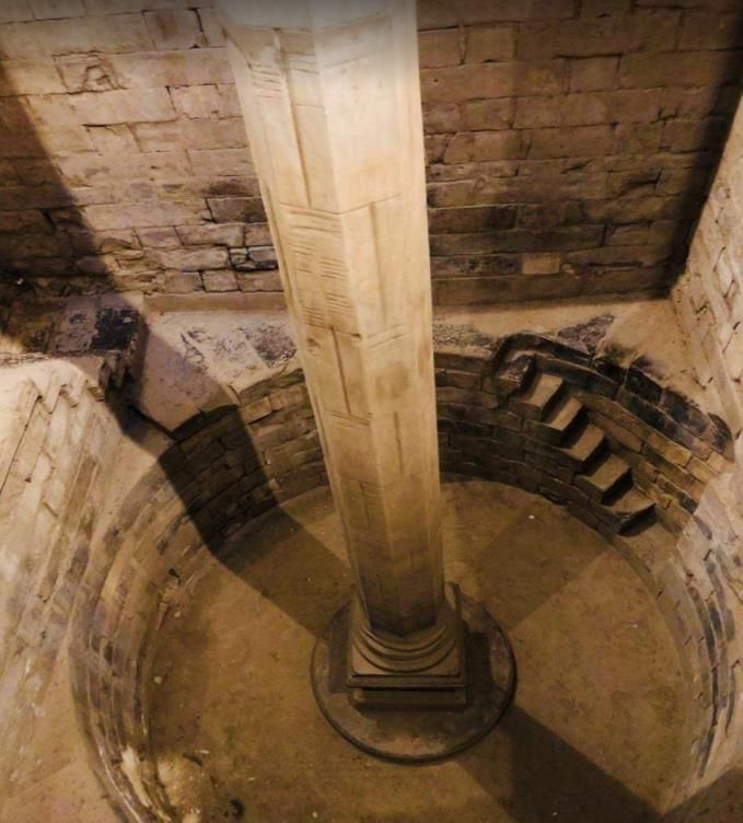
The Roda Nilometer and the longest instrumental record on Earth

 Photos by Loai Samen and
 Mohamd Mubarak; Google
 maps,
 https://goo.gl/maps/T8NUgo
 DAorK2 and
 https://goo.gl/maps/dsdJHJY
 Vv572.

The Roda Nilometer, near Cairo. Water entered through three tunnels and filled the Nilometer
chamber up to river level. The measurements were taken on the marble octagonal column (with
a Corinthian crown) standing in the centre of the chamber; the column is graded and divided into
19 cubits (each slightly more than 0.5 m) and could measure floods up to about 9.2 m. A
maximum level below the 16th mark could portend drought and famine and a level above the 19th
mark meant catastrophic flood.
 D. Koutsoyiannis, Climate of the past and present 40

Hurst-Kolmogorov (HK) dynamics and the perpetual change of
Earth’s climate 7

 Minimum water depth (m)
 Nile River annual minimum Annual
 6 30-year average water level (849 values)

 5

 4

 3

 2

 A hydroclimatic process 1
 as seen in the longest 0
 instrumental record 600 700 800 900 1000 1100 1200 1300 1400 1500
 Year AD
 7
 Minimum roulette wheel outcome

 "Annual" Each value is the minimum of m=36 roulette wheel
 6 30-"year" average outcomes. The value of m was chosen so that the standard
 A “roulette” process deviation be equal to the Nilometer series
 5

 4

 3

 2

 1

 0
 600 700 800 900 1000 1100 1200 1300 1400 1500
Nilometer data: Koutsoyiannis (2013) "Year"

 D. Koutsoyiannis, Climate of the past and present 41

The climacogram: A simple statistical tool to quantify
change across time scales
 ◼ Take the Nilometer time series, x1, x2, ..., x849, and calculate the sample estimate of
 variance γ(1), where the superscript (1) indicates time scale (1 year).
 ◼ Form a time series at time scale 2 (years):
 x1(2) := (x1 + x2)/2, x2(2) := (x3 + x4)/2, ..., x424 (2) := (x847 + x848)/2
 and calculate the sample estimate of the variance γ(2).
 ◼ Repeat the same procedure and form a time series at time scale 3, 4, … (years), up to
 scale 84 (1/10 of the record length) and calculate the variances γ(3), γ(4),… γ(84).
 ◼ The climacogram is a logarithmic plot of the variance γ(κ) vs. scale κ.
 ◼ If the time series xi represented a pure random process, the climacogram would be a
 straight line with slope –1 (the proof is very easy).
 ◼ In real world processes, the slope is different from –1, designated as 2H – 2, where H
 is the so-called Hurst parameter (0 < H < 1).
 ◼ The scaling law γ(κ) = γ(1) / κ2 – 2H defines the Hurst-Kolmogorov (HK) process.
 ◼ High values of H (> 0.5) indicate enhanced change at large scales, else known as long-
 term persistence, or strong clustering (grouping) of similar values.
Koutsoyiannis (2010, 2013, 2016)

 D. Koutsoyiannis, Climate of the past and present 42

The climacogram
 7

 Minimum water depth (m)
 Annual
 6 30-year average

of the Nilometer 5

 4

time series 3

 2

◼ The Hurst-Kolmogorov process 1
 seems consistent with reality. 0
 600 700 800 900 1000 1100 1200 1300 1400 1500
◼ The Hurst coefficient is H = 0.87. Year AD
 (Similar H values are estimated

 Bias
 The classical statistical estimator of standard
 from the simultaneous record of 1
 deviation was used, which however is biased
 maximum water levels and from for HK processes

 Variance (m²)
 the modern, 131-year, flow record
 of the Nile flows at Aswan).
◼ The Hurst-Kolmogorov behaviour,
 seen in the climacogram, indicates
 that:
 0.1
 (a) long-term changes are more
 frequent and intense than
 commonly perceived, and
 Empirical (from data)
 (b) future states are much more Purely random (H = 0.5)
 Markov
 uncertain and unpredictable on Hurst-Kolmogorov, theoretical (H = 0.87)
 long time horizons than 0.01
 Hurst-Kolmogorov adapted for bias

 implied by pure randomness. 1 10 100
 Scale (years)

 D. Koutsoyiannis, Climate of the past and present 43

A combined climacogram of temperature observations
 and proxies (Hurst-Kolmogorov + Milankovitch)
 1

 Orbital forcing
 20-100 kyears
 This slope NSSTC
 supports an HK CRU
Standard deviation (arbitrary units)

 behaviour with Moberg
 H > 0.92 Lohle
 Enhanced change Taylor
 GRIP
 EPICA
 Common perception: Slop
 Huybers
 Slop

 Purely random change e=- Zachos
 0.08
 Veizer
 e=

 Climate would stabilize
 -0.5

 in 30 years
 28 months

 The actual climatic variability at
 1 month

 the scale of 100 million years HK dynamics
 equals that of 28 months of a extends over all
 purely random climate! scales
 0.1
 10-2
 1.E-02 10-1
 1.E-01 100
 1.E+00 101
 1.E+01 102
 1.E+02 103
 1.E+03 104
 1.E+04 105
 1.E+05 106
 1.E+06 107
 1.E+07 108
 1.E+08
 Scale (years)
 Milankovitch’ theory explains only
Source: Markonis and Koutsoyiannis (2013) this “local” reduction of variance

 D. Koutsoyiannis, Climate of the past and present 44

Part 6
The energy cycle

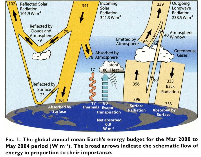
Global energy flows and energy balance

Trenberth et al.
(2009)

 D. Koutsoyiannis, Climate of the past and present 46

Comparison of human and natural locomotives
 (not to scale) Human locomotive
 All human energy
 production (2014):
 170 000 TWh/year
 = 0.612 × 1021 J/year
 = 0.612 ZJ/year (Mamassis
 et al., 2020)

 Natural locomotive
 Power density (for
 evaporating water):
 80 W/m2
 For earth’s area
 5.101× 1014 m2:
 4.08 × 1016 W = 40.8 PW
 Annual energy:
 1.290 × 1024 J/year
 = 1290 ZJ/year.
Image from http://4-designer.com/2014/03/Cartoon-steam-train-vector-material/ Koutsoyiannis (2020a)

 D. Koutsoyiannis, Climate of the past and present 47

Comparison of human and natural locomotives
(to scale)
 All human energy production
 Human
 locomotive
 0.612 ZJ/year

 Natural
 locomotive
 1290 ZJ/year
 (2100 times
 higher than all
 human energy
 production)

Image from http://4-designer.com/2014/03/Cartoon-steam-train-vector-material/ Koutsoyiannis (2020a)

 D. Koutsoyiannis, Climate of the past and present 48

Part 7
The carbon cycle

Anthropogenic changes
in atmospheric carbon
according to IPCC
(2013)
Questions:
1. Does the measured atmospheric
 growth rate (cyan in the lower
 part of the figure) originate from
 anthropogenic emissions as
 implied by the figure?
2. What percentage of the total
 carbon flow to the atmosphere
 do anthropogenic emissions From the original figure caption (IPCC, 2013)
 represent? Figure TS.4 | Annual anthropogenic CO2 emissions and
3. Is the net human effect on land their partitioning among the atmosphere, land and
 ocean (Gt / year; 1 Gt = 1 Pg) from 1750 to 2011. […].
 use increasing the emissions, as
 CO2 emissions from net land use change, mainly
 implied by the figure? deforestation, are based on land cover change data. […]

 D. Koutsoyiannis, Climate of the past and present 50

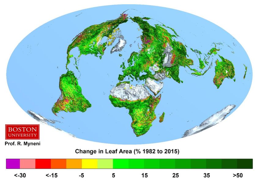
Quoting Zhu et al. (2016):
On question 3: “We show a persistent and
Is Earth browning or greening? widespread increase of
 growing season integrated
 LAI [Leaf Area Index]
 (greening) over 25% to 50%
 of the global vegetated
 area, whereas less than 4%
 of the globe shows
 decreasing LAI (browning).
 Factorial simulations with
 multiple global ecosystem
 models suggest that CO2
 fertilization effects explain
 70% of the observed
 greening trend, followed by
 nitrogen deposition (9%),
 climate change (8%) and
 land cover change (LCC)
 (4%). CO2 fertilization effects
 explain most of the greening
Image source: http://sites.bu.edu/cliveg/files/2016/04/LAI-Change.png trends in the tropics […]”
 D. Koutsoyiannis, Climate of the past and present 51

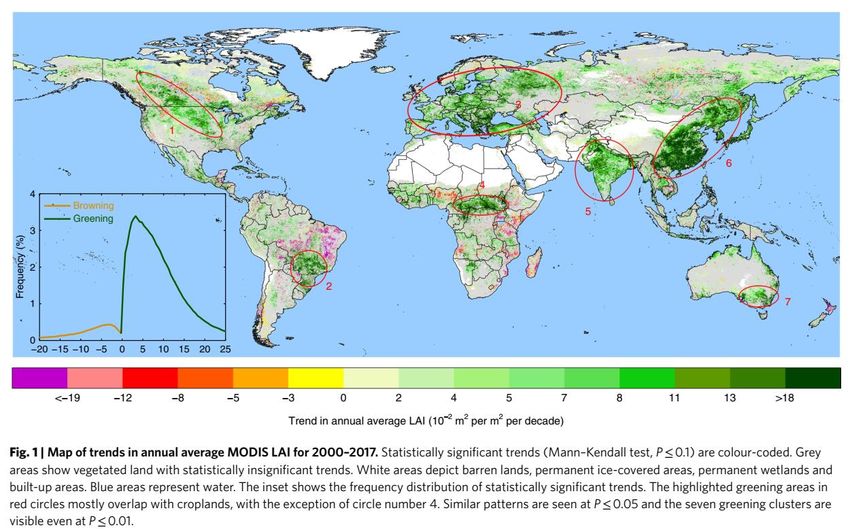
On question 3: Are human activities browning or
greening the Earth?
 Source: Chen
 et al. (2019)

Quoting Chen et al. (2019): “recent satellite data (2000–2017) reveal a greening pattern
that is strikingly prominent in China and India and overlaps with croplands world-wide.”
 D. Koutsoyiannis, Climate of the past and present 52

On question 2: Synthesis of the atmospheric carbon
balance
 Photosynthesis -123
 Terrestial

 Respiration 59.8
 Decay 53.9
 Fire 5
 Freshwater outgassing 1
 Volcanism & weathering 0.4
 Human Maritime

 Absorption and photosynthesis -80
 Respiration 78.4

 Fossil fuels & cement production 7.8
 Land use change 1.1
 Outflows: -203 Gt C / year Inflows: 207.4 Gt C / year
 -140 -120 -100 -80 -60 -40 -20 0 20 40 60 80 100
 Average increase of atmospheric CO₂
 CO₂ flux (Gt C / year)
 concentration: 4.4 Gt C / year

Totals according to IPCC (2013) and additional information from Green and Byrne (2004).

 D. Koutsoyiannis, Climate of the past and present 53

On question 2: Percentage of the anthropogenic
emissions on total carbon flux to the atmosphere
 Human CO₂ emissions
 (fossil fuels and
 cement production):
 3.8%

 Natural CO₂ emissions
 (respiration, decay,
 etc., in land and sea):
 96.2%

 Areas plotted to scale

Images from: https://www.whitehorse.vic.gov.au/dust-smoke-fumes-and-odour-nuisance
https://www.wallpapers13.com/tropical-landscape-marine-animal-underwater-world-sea-dolphin-colorful-sea-fish-corals-land-coast-
palm-trees-scarlet-birds-sunrise-art-wallpaper-hd-1920x1200/

 D. Koutsoyiannis, Climate of the past and present 54

On Question 1: Covid-19 and an unfortunate experiment

 0.5
 0.25
Gt CO2/year

 Gt C/year
 0
 0.25
 0.5
 418
 2020 0.75
 416 2019
 CO₂ concentration (ppm)

 2018
 414
 2017 ◼ The global CO2 emissions
 412
 were over 5% lower in the
 410 first quarter of 2020 than
 408 in that of 2019 (IEA, 2020).
 406 ◼ However, the increasing
 404 pattern of atmospheric
 402
 CO2 concentration, as
 1 2 3 4 5 6 7 8 9 10 11 12 measured in Mauna Loa,
 Month did not change.
 Koutsoyiannis and Kundzewicz (2020)

 D. Koutsoyiannis, Climate of the past and present 55

Causation between CO₂ and temperature:
“ὄρνις ἢ ᾠὸν;” (“hen or egg?”)1

 T↗ CO₂↗

 Koutsoyiannis and Kundzewicz (2020)

Koutsoyiannis and Kundzewicz (2020) postulate that the link between CO₂ and
temperature classifies as a “hen-or-egg” causality problem, as it is not clear
which of two is the cause and which the effect.
1Plutarch first posed this type of causality as a philosophical problem using the example of the hen
and the egg: “Πότερον ἡ ὄρνις πρότερον ἢ τὸ ᾠὸν ἐγένετο” (Πλούταρχος, Ηθικά, Συμποσιακὰ Β,
Πρόβλημα Γ) —Which of the two came first, the hen or the egg? (Plutarch, Moralia, Quaestiones
convivales, B, Question III).

 D. Koutsoyiannis, Climate of the past and present 56

4 320
Palaeoclimatic data T CO₂

 Temperature difference from present
 2 300

in search of causality

 CO₂ concetration (ppmv)
 0 280

 -2 260
Time series of temperature and CO₂ -4 240
concentration from the Vostok ice
 -6 220
core, covering part of the
Quaternary (420 000 years) with -8 200
time step of 1000 years. -10 180
 400000 300000 200000 100000 0
 Years before present
Auto- and cross-correlograms of 1
the two time series. The maximum T
value of the cross-correlation 0.8 CO₂
 T - CO₂

 Correlation coefficient
coefficient is 0.88 and appears at lag 0.6
1 thousand years. 0.4

 0.2
This suggests that the dominant
 0
causality direction is T → CO₂ and that
Milankovitch, rather than Arrhenius, is -0.2

right. -0.4
 -40 -30 -20 -10 0 10 20 30 40
Adapted from Koutsoyiannis (2019) Lag (thousand years)

 D. Koutsoyiannis, Climate of the past and present 57

Recent 1
 0.8
 ΔΤ Δln[CO₂]
 0.01

instrumental 0.6
 0.4
 0.008

temperature

 Δln[CO₂]
 0.2 0.006

 ΔT
and CO₂ data 0
 -0.2 0.004

Differenced monthly time -0.4

series of global temperature -0.6 0.002

(UAH) and logarithm of CO₂ -0.8

concentration (Mauna Loa) -1 0
 1980 1985 1990 1995 2000 2005 2010 2015 2020
Annually averaged time series of 0.4
 ΔΤ
 0.009
differenced temperatures (UAH) and 0.3 Δln[CO₂] 0.008
logarithm of CO₂ concentration
 0.2 0.007
(Mauna Loa). Each dot represents
the average of a one-year duration 0.1 0.006

 Δln[CO₂]
ending at the time of its abscissa.
 ΔT

 0 0.005

 -0.1 0.004
Which is the cause and which the
effect? -0.2 0.003

 -0.3 0.002
Koutsoyiannis and Kundzewicz (2020); notice that
logarithms of CO₂ concentration are used for -0.4 0.001
linear equivalence with temperature. 1980 1985 1990 1995 2000 2005 2010 2015 2020

 D. Koutsoyiannis, Climate of the past and present 58

1 ΔΤ
 Changes in CO₂ 0.8
 Δln[CO₂]
 ΔΤ - Δln[CO₂], monthly

 follow changes in ΔΤ - Δln[CO₂], annual

 Correlation coefficient
 0.6 ΔΤ - Δln[CO₂], fixed year

 global temperature 0.4

 Auto- and cross-correlograms of the 0.2

 differenced time series of 0
 temperature (UAH) and logarithm of
 CO₂ concentration (Mauna Loa) -0.2

 Which is the cause and which -0.4
 -48 -36 -24 -12 0 12 24 36 48
 the effect? Lag (months)

 Maximum cross-correlation coefficient (MCCC) and corresponding time lag in months
 Monthly time Annual time series – Annual time series –
 series sliding annual window fixed annual window
 Temperature - CO₂ series MCCC Lag MCCC Lag MCCC Lag
 UAH – Mauna Loa 0.47 5 0.66 8 0.52 12
 UAH – Barrow 0.31 11 0.70 14 0.59 12
 UAH – South Pole 0.37 6 0.54 10 0.38 12
Koutsoyiannis UAH – Global 0.47 6 0.60 11 0.60 12
and
Kundzewicz CRUTEM4 – Mauna Loa 0.31 5 0.55 10 0.52 12
(2020) CRUTEM4 – Global 0.33 9 0.55 12 0.55 12

 D. Koutsoyiannis, Climate of the past and present 59

Towards a physical explanation for causality direction
◼ We start from the Arrhenius equation for the rate of chemical reactions (which should
 not be confused with the Arrhenius climate theory):

 = exp −
 
 where k is the rate constant of the chemical reaction, T is the absolute temperature
 (in kelvins), A is a constant, E is the activation energy and R is the universal gas
 constant.
◼ Assuming = 0 + Δ for some 0 > 0 for which = 0 and for Δ ≪ 0 , we can
 write:
 Δ Δ 
 = exp − + = exp − ≈ exp −
 0 0 + Δ 0 0 + Δ 0 0 0
◼ Hence:
 Δ 1
 0 0
 ≈ 0 = 0 Δ , where ≔
 0 0
 This is an exponential function of Δ .

 D. Koutsoyiannis, Climate of the past and present 60

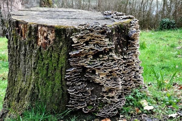
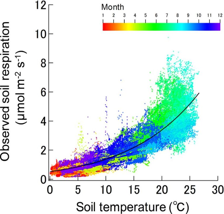
Physical explanation of the T → CO₂ causality
◼ The approximation of the Arrhenius equation for the
 rate of chemical reactions, i.e.:
 ≈ 0 Δ Makita et al. (2018, Fig. 2)
 remains valid for biochemical and biological
 processes (for typical temperature ranges).
◼ Thus, the graph on the right for the respiration rate
 s (emission of CO₂ from plants and microorganisms)
 of a coniferous forest can be modelled as:
 s = 2.18 1.09 −15
◼ This entails a 9% increase of respiration for an
 increase of temperature by 1 °C (= 1 K).
◼ Also, it has been known since 70 years ago (Pomeroy
 and Bowlus, 1946) that the metabolic rate (activity of
 microorganisms) in sewer networks follows similar
 dynamics, i.e.:
 EBOD = BOD 1.07 −20 Graph reproduced from Makita et al.
 where BOD stands for biochemical oxygen demand (2018) showing the relationship between
 and EBOD for effective BOD. soil respiration and temperature during
◼ The latter equation (routinely used in engineering 2005-10 in a temperate evergreen
 design even today) suggests a 7% increase of coniferous forest area in Japan. The best-
 metabolic rate for temperature increase of 1 °C. fit model is shown by the solid black line.
 D. Koutsoyiannis, Climate of the past and present 61

How does the natural increase of respiration
compare to human emissions?
◼ The soil respiration, assumed to be the sum of respiration (plants) and decay
 (microbes) is 113.7 Gt C/year (see graph of atmospheric carbon balance).
◼ According to Koutsoyiannis (2020, Table 2), in the last 30 years the land
 temperature has been increasing by 0.29 °C/decade, corresponding to an
 increase in temperature over land of 1.16 °C for the 40-year period 1980 –
 2020.
◼ This means that between 1980 and 2020 there was an increase of annual
 respiration and decay over land, amounting to 11% or 12 Gt C/year.
◼ This annual increase is by 50% higher than human emissions (7.8 Gt/year as
 shown in the graph of atmospheric carbon balance).
◼ We can expect that the sea
 respiration would have increased
 too, but at a lower rate as the
 sea temperature increase is much T↗ CO₂↗
 lower.

 D. Koutsoyiannis, Climate of the past and present 62

Part 8
The hydrological cycle
and its alleged intensification

The hydrological cycle: A recent quantification
 Koutsoyiannis (2020a)

 Notice the
 groundwater
 depletion, i.e.,
 Condensation (unsustainable)
 over pumping
 Advection (net), A beyond the rate of
 31 900 km3/year natural recharge.
 This contributes

 399 400 km3/year
 (1094 mm/year)
 123 300 km3/year

 Precipitation, PS
 (+ transpiration) , EL
 Precipitation, PL

 (850 mm/year)

 431 300 km3/year
 1/3 of the sea-

 (1182 mm/year)
 91 400 km3/year
 (630 mm/year)

 Evaporation, ES
 Evaporation
 level rise—the
 most significant
 anthropogenic
 effect on the
 hydrological cycle.
 Surface runoff, R
 Another 1/3 is
 32 000 km3/year contributed by ice
 (219 mm/year) Climatic variability
 (30-year scale, 95% confidence) loss (not
 Precipitation and evaporation: ±7% necessarily
 Runoff and advection: ±23%
 depletion, dSG/dt

 anthropogenic),
 (2.1 mm/year)
 300 km3/year
 Groundwater

 Groundwater discharge, G while 1/3 is due to
 500 km3/year
 (3.4 mm/year) thermal
 expansion.

 D. Koutsoyiannis, Climate of the past and present 64

Dew point and its comparison to temperature
 ◼ The presence of water in the atmosphere (and hence hydrology) is affected more by
 the dew point, Td, than the temperature, T.
 ◼ The dew point is defined as the temperature at which the air must be cooled to
 become saturated with water vapour; thus when the relative humidity is 100%, the
 dew point equals the temperature.
 1.6
 Zonal distribution of the
Difference from 1980-1999 average (°C)

 Temperature, T
 1.4 difference of the earth
 Dew point, T_d
 temperature and dew point from
 1.2
 their averages in the 20-year
 1 period 1980-99, from ERA5
 reanalysis data. Note that the
 0.8 Polar Temperate Tropical Temperate graph represents averages for the
 0.6 entire 40+ year period 1980-
 2019, rather than differences
 0.4 between two periods (the latter
 Polar
 0.2 are about twice the former).
 0 Notice the zero change in the
 dew point in the tropics, which
 -0.2 are responsible for most part of
 -90 0 -60
 30 -30
 60 90 evaporation.
 Latitude (°)
 Koutsoyiannis (2020a); Reanalysis data access and processing through http://climexp.knmi.nl

 D. Koutsoyiannis, Climate of the past and present 65

1000

Saturation vapour pressure Proposed

 Saturation vapour pressure (hPa)
 Standard solution of Clausius-Clapeyron
 100

and humidity 10

◼ The saturation vapour pressure, , increases almost
 exponentially with temperature, T: 1

 L − / 
 0 0 0.1
 = = 0 exp 1− -40 -30 -20 -10 0 10 20 30 40 50
 0 
 Temperature (°C)
 5.06
 0 0
 = 0 exp 24.921 1 −
 
 where (T0, e0) are the coordinates of the triple point of
 water, R is the specific gas constant of water vapour, cp is
 the specific heat at constant pressure of the vapour and cL is
 the specific heat of the liquid water.
◼ The dew point is ≔ −1 ( A ), where A is the actual
 vapour pressure, and the relative humidity is the ratio: The law was derived by studying
 A ( d ) a single molecule and maximizing the
 ≔ = combined uncertainty of its state, i.e.:
 ( )
◼ The specific humidity is the ratio of the density of vapour (a) its phase (whether gaseous or liquid);
 v to the density of air v + d , where d is the density of (b) its position in space; and
 dry air, and is related to vapour pressure by: (c) its kinetic state, i.e., its velocity and
 v A other coordinates corresponding to its
 ≔ = degrees of freedom and making up its
 v + d − 1 − A
 thermal energy.
 where ε =0.622 is the ratio of the molecular mass of water
 to that of the mixture of gases in the dry air. Koutsoyiannis (2012, 2014a)

 D. Koutsoyiannis, Climate of the past and present 66

Basic assumptions of IPCC on hydrological cycle
◼ As a result of increasing temperature, the saturation vapour pressure is increasing by
 6%–7% per °C of warming.
 ❑ This is a fact resulting from the Clausius–Clapeyron relationship and does not need
 observations to confirm.
◼ In a warming climate, atmospheric moisture is changing in a manner that the relative
 humidity remains constant, but specific humidity increases according to the Clausius–
 Clapeyron relationship. As a result, the established view is that the global atmospheric
 water vapour should increase by about 6%–7% per °C of warming.
 ❑ This is a conjecture that needs to be tested by data.

◼ This gives rise to what has been called intensification of hydrological cycle.
 ❑ Because of the alleged intensification, the role of hydrology becomes thus
 important in the climate agenda from a sociological point of view: some of the
 most prominent predicted catastrophes are related to water shortage and extreme
 floods (Koutsoyiannis, 2014b).
◼ The rate of increase of precipitation, necessarily accompanied by an equal rate of
 increase of evaporation, estimated from climate model simulations, is conjectured to
 be smaller, 1% to 3% per °C, with a typical estimate of 2.2% per °C (Kleidon and
 Renner, 2013).
 ❑ Even accepting this IPCC assertion and the celebrated target of 2 °C of global
 warming, which translates in 2-6% increase of rainfall, the change is negligible.
 D. Koutsoyiannis, Climate of the past and present 67

Decadal change as seen in a long daily precipitation record
All 10-year 200 4
climatic indices Daily 10-year high, KM

 Precipitation, daily & 10-year high daily (mm)
 180 10-year high, OS 10-year average 3.6
have varied

 Precipitation. 10-year average daily (mm)
 10-year probability wet
substantially and 160 1933: 155.7 mm 3.2
irregularly:

 Probability wet x 10 (-)
The average by 140 2.8
100% (from 1.2 120 2.4
to 2.4 mm).
 100 2
The probability
wet by 120% 80 1.6
(from 0.15 to
 60 1.2
0.33).
The high daily 40 0.8
precipitation by 20 0.4
150% (from 44 to
110 mm/d). 0 0
Why hydrologists 1800 1850 1900 1950 2000
have given so
much energy in Bologna, Italy (44.50°N, 11.35°E, +53.0 m). Available from the Global Historical Climatology
studying impacts Network (GHCN) – Daily (https://climexp.knmi.nl/gdcnprcp.cgi?WMO=ITE00100550).
a priori framed Uninterrupted for the period 1813-2007: 195 years. For the period 2008-2018, daily data are
within 2-6%? provided by the repository Dext3r of ARPA Emilia Romagna. Total length: 206 years.

 D. Koutsoyiannis, Climate of the past and present 68

Saturation vs. actual water vapour pressure
 ◼ The graph shows the variation of the water vapour pressure, saturation, e(T),
 (continuous lines) and actual, e(Td), (dashed lines) for the average temperature T and
 dew point Td.
 ◼ Clearly, the increase in e(Td) is smaller than that in e(Td), thus falsifying the constant
 relative humidity conjecture of IPCC.
 ◼ In particular, in land, where hydrological processes mostly occur, there is no increase
 in e(Td), while there is in e(T).
 20 20 20
 Land
Vapour pressure, e(T), e(T₋d) (hPa)

 Vapour pressure, e(T), e(T₋d) (hPa)
 Vapour pressure, e(T), e(T₋d) (hPa)
 18 18 18

 16 16 16

 14 14 14

 12 12 12

 10 10 10

 8 8 8

 6 6 6
 Earth Sea
 4 4 4
 1985

 2010
 1975
 1980

 1990
 1995
 2000
 2005

 2015
 2020

 1975
 1980
 1985
 1990
 1995
 2000
 2005
 2010
 2015
 2020
 1975
 1980
 1985
 1990
 1995
 2000
 2005
 2010
 2015

Source of graph: Koutsoyiannis (2020a); source of Thin and thick lines of the same colour represent monthly 2020
data: ERA5 reanalysis, http://climexp.knmi.nl values and running annual averages (right aligned), respectively.

 D. Koutsoyiannis, Climate of the past and present 69

850 hPa (~1500 m) 300 hPa (~9000 m)
Specific 9 0.35

 Specific humidity (g/kg)

 Specific humidity (g/kg)
 8
humidity: 7
 6
 0.3

 0.25

Does it 5
 4
 0.2

increase? 3
 2
 NCEP-NCAR
 ERA5 Earth
 0.15

 0.1
 1940 1950 1960 1970 1980 1990 2000 2010 2020 1940 1950 1960 1970 1980 1990 2000 2010 2020
◼ The specific 9 0.35
 humidity is Specific humidity (g/kg)

 Specific humidity (g/kg)
 8
 0.3
 7
 fluctuating— 0.25
 6
 not increasing 5 0.2
 monotonically. 4
 NCEP-NCAR 0.15
 3
◼ Hence, the IPCC 2 ERA5 Land
 0.1
 Land
 conjecture is 1940 1950 1960 1970 1980 1990 2000 2010 2020 1940 1950 1960 1970 1980 1990 2000 2010 2020
 falsified. 9 0.35
 Specific humidity (g/kg)

 Specific humidity (g/kg)
 8
 0.3
◼ Interestingly, in 7
 the NCEP-NCAR 6 0.25
 5
 reanalysis at the 0.2
 4
 300 hPa, the 3
 NCEP-NCAR 0.15
 ERA5 Sea Sea
 specific humidity 2 0.1
 is decreasing. 1940 1950 1960 1970 1980 1990 2000 2010 2020 1940 1950 1960 1970 1980 1990 2000 2010 2020

Source of graph: Koutsoyiannis (2020a); data: NCEP- Thin and thick lines of the same colour represent monthly
NCAR & ERA5 reanalysis, http://climexp.knmi.nl values and running annual averages (right aligned), respectively.

 D. Koutsoyiannis, Climate of the past and present 70