Monitoring aerosols over Europe: an assessment of the potential benefit of assimilating the VIS04 measurements from the future MTG/FCI ...
←
→
Page content transcription
If your browser does not render page correctly, please read the page content below
Atmos. Meas. Tech., 12, 1251–1275, 2019
https://doi.org/10.5194/amt-12-1251-2019
© Author(s) 2019. This work is distributed under
the Creative Commons Attribution 4.0 License.

Monitoring aerosols over Europe: an assessment of the potential
benefit of assimilating the VIS04 measurements from the future
MTG/FCI geostationary imager
Maxence Descheemaecker1 , Matthieu Plu1 , Virginie Marécal1 , Marine Claeyman2 , Francis Olivier2 , Youva Aoun3 ,
Philippe Blanc3 , Lucien Wald3 , Jonathan Guth1 , Bojan Sič1 , Jérôme Vidot4 , Andrea Piacentini5 , and Béatrice Josse1
1 CNRM,  Université de Toulouse, Météo-France, CNRS, Toulouse, France
2 ThalesAlenia Space, Cannes la Bocca, 06156, France
3 Mines ParisTech, PSL Research University, O.I.E. – Center for Observation, Impacts, Energy,

Sophia Antipolis, 06904, France
4 CNRM, Université de Toulouse, Météo-France, CNRS, Lannion, France
5 CERFACS – CNRS, UMR5318, 31057, Toulouse, France

Correspondence: Matthieu Plu (matthieu.plu@meteo.fr)

Received: 2 July 2018 – Discussion started: 6 August 2018
Revised: 2 January 2019 – Accepted: 7 February 2019 – Published: 27 February 2019

Abstract. The study assesses the possible benefit of assim-        sensor to bring added value to the MOCAGE aerosol simu-
ilating aerosol optical depth (AOD) from the future space-         lations, and in general, to other chemistry transport models.
borne sensor FCI (Flexible Combined Imager) for air quality
monitoring in Europe. An observing system simulation ex-
periment (OSSE) was designed and applied over a 4-month
period, which includes a severe-pollution episode. The study       1   Introduction
focuses on the FCI channel centred at 444 nm, which is the
shortest wavelength of FCI. A nature run (NR) and four             Aerosols are liquid and solid compounds suspended in the
different control runs of the MOCAGE chemistry transport           atmosphere, which have sizes ranging from a few nanome-
model were designed and evaluated to guarantee the robust-         tres to several tens of micrometres and lifetimes in the tro-
ness of the OSSE results. The synthetic AOD observations           posphere varying from a few hours to a few weeks (Seinfeld
from the NR were disturbed by errors that are typical of the       and Pandis, 1998). Stable sulfate aerosols at high altitude can
FCI. The variance of the FCI AOD at 444 nm was deduced             last for years (Chazette et al., 1995). The sources of aerosols
from a global sensitivity analysis that took into account the      may be natural (dust, sea salt, ashes from volcanic eruptions,
aerosol type, surface reflectance and different atmospheric        for instance) or anthropogenic (from road traffic, residential
optical properties. The experiments show a general benefit to      heating, industries, for instance), and they can be transported
all statistical indicators of the assimilation of the FCI AOD at   up to thousands of kilometres. Aerosols are known to have
444 nm for aerosol concentrations at the surface over Europe,      significant impacts on climate (IPCC, 2007) and on air qual-
and also a positive impact during the severe-pollution event.      ity and further on human health as WHO (2016) estimated
The simulations with data assimilation reproduced spatial          over 3 million deaths in 2012 to be due to aerosols.
and temporal patterns of PM10 concentrations at the surface           Aerosols absorb and diffuse solar radiation, which leads to
better than those without assimilation all along the simula-       local heating of the aerosol layer and cooling of the climate
tions and especially during the pollution event. The advan-        system through the backscatter of solar radiation to space for
tage of assimilating AODs from a geostationary platform            most of the aerosols, except for black carbon (Stocker et al.,
over a low Earth orbit satellite has also been quantified. This    2013). The absorption of solar radiation modifies the vertical
work demonstrates the capability of data from the future FCI       temperature profile, affecting the stability of the atmosphere

Published by Copernicus Publications on behalf of the European Geosciences Union.
1252                                                                M. Descheemaecker et al.: Monitoring aerosols over Europe

and cloud formation (Seinfeld and Pandis, 1998). Aerosols,            Different AODs are retrieved over lands from SEVIRI data
as condensation nuclei, play a significant role in the forma-         in the VIS0.6 and VIS0.8 channels, respectively centred at
tion and life cycle of clouds (Seinfeld and Pandis, 1998).            0.635 µm (0.56–0.71 µm) and 0.81 µm (0.74–0.88 µm). AOD
Deposition of aerosols on the Earth’s surface may also af-            products are retrieved following different methods. Carrer et
fect surface properties and albedo. All these effects show that       al. (2010) presented a method to estimate a daily quality-
aerosols play a key role on the energy budget of the climate          controlled AOD based on a directional and temporal analyses
system.                                                               of SEVIRI observations of channel VIS0.6. Another method
   Aerosols, also called particulate matter in the context of air     consists of matching simulated top-of-the-atmosphere (TOA)
quality, are responsible for serious health problems all over         reflectances (from a set of five models) with TOA SEVIRI
the world, as they are known to favour respiratory and cardio-        reflectances (Bernard et al., 2011) to obtain an AOD for
vascular diseases as well as cancers (Brook et al., 2004). The        VIS0.6. Another method (Mei et al., 2012) estimates the
World Health Organization (WHO) has set regulatory lim-               AOD and the aerosol type by analysing the reflectances at
its for aerosol concentrations, which are annual means of 20          0.6 and 0.8 µm in three orderly scan times. These methods
and 10 µg m−3 for PM10 and PM2.5 (particulate matter with             derive AODs for specific channels from the combined analy-
diameters less than 10 and 2.5 µm, respectively) concentra-           sis of the data from several channels and from multiple times.
tions. The European Union regulation also introduces PM10                Numerical models, even if they are subject to errors, are
daily mean limits of 50 µg m−3 . The presence of a dense              necessary to describe the variability of the aerosol types
layer of aerosols can also affect air traffic by the reduction        and their concentrations with space and time, as a comple-
in visibility (Bäumer et al., 2008) and by risking disruption         ment to the observations. Aerosol forecasts on regional and
in the engines of aeroplanes (Guffanti et al., 2010). There-          global scales are made by three-dimensional models, such as
fore, it is essential to accurately determine the evolution of        the chemistry transport model (CTM) MOCAGE (Sič et al.,
the concentration and size of the different types of aerosols         2015; Guth et al., 2016). MOCAGE is currently used daily to
in space and time in order to assess their effect on climate          provide air quality forecasts to the French platform Prev’Air
and on air quality and to mitigate their impacts. A pertinent         (Rouil et al., 2009) and also to the European CAMS ensem-
approach to achieving a continuous and accurate monitoring            ble (Marécal et al., 2015). Data assimilation of AOD can
of aerosols is to combine measurements and models, a good             be used in order to improve the representation of aerosols
example being the Copernicus Atmosphere Monitoring Ser-               within the model simulations (Benedetti et al., 2009, Sič et
vice (CAMS) (https://atmosphere.copernicus.eu, last access:           al., 2016). Studies on geostationary sensors have also proved
19 February 2019; Peuch and Engelen, 2012; Eskes et al.,              to have a positive effect of the assimilation of AOD; see e.g.
2015; Marécal et al., 2015).                                          Yumimoto, et al. (2016), who assessed this positive effect
   Ground-based stations, which measure aerosol and gas               using the AOD at 550 nm from AHI (Advanced Himawari
concentrations in situ, have been used for several decades            Imager) sensor aboard Himawari-8.
to monitor air quality, such as the stations in the Air Qual-            The future geostationary Flexible Combined Imager (FCI,
ity e-Reporting programme (EEA, 2019) from the European               Eumetsat, 2010), which will be aboard the Meteosat Third
Environment Agency (EEA). Other observations can also be              Generation satellite (MTG), will perform a full disk in
used to measure aerosols. The AERONET (AErosol RObotic                10 min, and in 2.5 min for the European Regional-Rapid-
NETwork) programme (NASA, 2019) performs the retrieval                Scan, which covers one-quarter of the full disk, with a spa-
of the aerosol optical depth (AOD) at several ground sta-             tial resolution of 1 km at nadir and around 2 km in Europe.
tions (Holben et al., 1998). Similarly, AOD observations              Like AHI, FCI is designed to have multiple wavelengths and
can be retrieved from images taken in different channels              the assimilation of its data into models should be beneficial
by imagers aboard low Earth orbit (LEO) or GEOstation-                to aerosol monitoring. The aim of the paper is to assess the
ary (GEO) satellites. Generally, AOD from satellite provides          possible benefit of assimilating measurements from the fu-
a better spatial coverage than ground-based stations at the           ture MTG/FCI sensor for monitoring aerosols on a regional
expense of additional sources of uncertainty, such as the             scale over Europe. Since MOCAGE cannot assimilate AODs
surface reflectance. For example, daily AOD products are              at multiple wavelengths simultaneously (Sič et al., 2016),
derived from the Moderate Resolution Imaging Spectrora-               the study focuses on the assimilation of AODs from a sin-
diometer (MODIS) (Levy et al., 2013) sensor on board Terra            gle channel. Among the 16 channels of FCI, the VIS04 band
and Aqua LEO satellites: AOD products at 10 km resolu-                (centred at 444 nm) has been chosen because it covers the
tion (MOD 04 and MYD 04 products) or at 1 km resolu-                  shortest wavelengths, which is expected to be the most rele-
tion (MAIAC product). Sensors on geostationary orbit satel-           vant to detect small particles (Petty, 2006). Besides, VIS04 is
lites can continuously scan one-third of the Earth’s surface          a new channel compared to MSG/SEVIRI, the shortest band
much more frequently than low Earth orbit satellites. The SE-         of which is around 650 nm (Carrer et al., 2010), and so as-
VIRI (Spinning Enhanced Visible and Infrared Imager) sen-             sessing the benefit of VIS04 over Europe is original.
sor, aboard MSG (Meteosat Second Generation), is an ex-                  As FCI is not yet operational, an OSSE (Observing Sys-
ample of a GEO sensor providing information on aerosols.              tem Simulation Experiments) approach (Timmermans et al.,

Atmos. Meas. Tech., 12, 1251–1275, 2019                                                 www.atmos-meas-tech.net/12/1251/2019/
M. Descheemaecker et al.: Monitoring aerosols over Europe                                                                       1253

2015) is used in this study. In an OSSE, synthetic observa-
tions are created from a numerical simulation that is as close
as possible to the real atmosphere (the nature run) and then
are assimilated in a different model configuration. The dif-
ferences between model outputs with and without assimila-
tion provide an assessment of the added value of the assim-
ilated data. OSSE have been widely developed and used for
assessing and designing future sensors for air quality moni-
toring: for carbon monoxide (Edwards et al., 2009; Abida et
al., 2017) and ozone (Claeyman et al., 2011; Zoogman et al.,
2014) from LEO or GEO satellites (Lahoz et al., 2012), and
for aerosol analysis from GEO satellites over Europe (Tim-
mermans et al., 2009a, b). Some of these studies have suc-
cessfully assessed the potential benefit of future satellites and
they have helped to design the instruments (Claeyman et al.,
2011). However cautions and limitations on the OSSE for air
quality have been addressed (Timmermans et al., 2009a, b,
2015), such as the “identical twin problem” and the control
over the boundary conditions of the model, and the accuracy
and the representativeness of the synthetic observations.           Figure 1. Schematic representation of the OSSE principle.
   By designing an OSSE that takes into account these pre-
cautions, the present study proposes a quantitative assess-
                                                                    differences between AR and CR quantify the added value of
ment of the potential benefit of assimilating AOD at 444 nm
                                                                    the instrument.
from FCI for aerosol monitoring in Europe. The OSSE and
                                                                       The NR should be as close as possible to the actual at-
its experimental set-up are described in Sect. 2. Then, the
                                                                    mosphere because it serves as a reference for producing the
case study and an evaluation of the ability of the reference
                                                                    synthetic observations. The temporal and spatial variations of
simulation to represent a true state of the atmosphere are pre-
                                                                    the NR should approximate those of actual observations. An
sented. The calculation of synthetic observations is explained
                                                                    evaluation of the NR, presented in Sect. 2.2, includes a com-
in Sect. 3. An evaluation of the control simulations is made
                                                                    parison of the model with aerosol concentrations and AOD
in Sect. 4. In Sect. 5, the results of the assimilation of FCI
                                                                    data from ground-based stations.
synthetic observations are presented and discussed. Finally,
                                                                       In addition, the differences between the NR and the CR
Sect. 6 concludes this study.
                                                                    must be significant and approximate those between the CR
                                                                    and the actual observations. Ideally, the NR and CR should
                                                                    be run with different models, as the use of the same model
2     Methodology                                                   could lead to over-optimistic results (Masutani et al., 2010);
                                                                    this issue is called the identical twin problem. It is strongly
2.1    Experimental set-up                                          recommended that the spatio-temporal variability of the NR
                                                                    and its differences should be evaluated with the CR to avoid
                                                                    this problem (Timmermans et al., 2015). As MOCAGE is
Figure 1 shows the general principle of the OSSE (Timmer-
                                                                    used for both NR and CR in the present study, a method sim-
mans et al., 2015). A reference simulation, called “nature
                                                                    ilar to that used in Claeyman et al. (2011) is proposed. Instead
run” (NR) is assumed to represent the “true” state of the
                                                                    of one CR, various CR simulations (Fig. 1) are performed
atmosphere. Synthetic AOD observations are generated by
                                                                    in different configurations, and they are assessed indepen-
combining AOD retrieved from the NR and the error char-
                                                                    dently and compared to the NR to ensure the robustness of
acteristics of FCI. These error characteristics are described
                                                                    the OSSE results. An evaluation of those differences is pre-
in Sect. 3. The second kind of simulations in the OSSE is
                                                                    sented in Sect. 4.
the control run (CR) simulation. The differences between NR
output and CR output should represent the errors of current
models without the use of observations. Finally, the assimi-
lation run (AR) is done by assimilation in the CR of the syn-
thetic observations. To assess the added value of the instru-
ment, a comparison is made between the output of the AR
and the NR and between the CR and the NR. If the AR is
closer to the NR than the CR, it means that the observations
provide useful information for the assimilation system. The

www.atmos-meas-tech.net/12/1251/2019/                                                 Atmos. Meas. Tech., 12, 1251–1275, 2019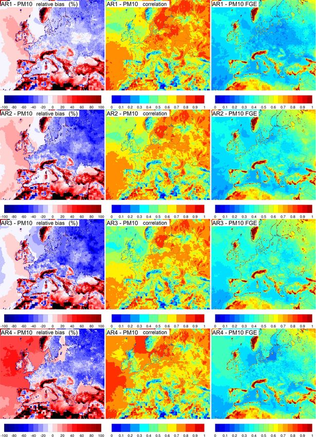
1254                                                             M. Descheemaecker et al.: Monitoring aerosols over Europe

2.2    MOCAGE                                                      scheme (Williamson and Rasch, 1989), a parameterization
                                                                   for convection (Bechtold et al., 2001) and a diffusion scheme
The CTM model used in this study is MOCAGE (Modèle de              (Louis, 1979) are used to transport gaseous and particulate
Chimie Atmosphérique à Grande Echelle, Guth et al., 2016),         species.
which has been developed for operational and research pur-
poses. MOCAGE is a three-dimensional model that cov-               2.3   Assimilation system PALM
ers the global scale, down to regional scale using two-way
nested grids. MOCAGE vertical resolution is not uniform:           The assimilation system of MOCAGE (Massart et al., 2009),
the model has 47 vertical sigma-hybrid altitude-pressure lev-      is based on the 3-dimensional first guess at appropriate time
els from the surface up to 5 hPa. Levels are denser near the       (3D-FGAT) algorithm. This method consists of minimizing
surface, with a resolution of about 40 m in the lower tropo-       the cost function J :
sphere and 800 m in the lower stratosphere.                                                      1
   MOCAGE simulates gases (Josse, 2004; Dufour et al.,             J (δx) = Jb (δx) + Jo (δx) = (δx)T B−1 δx
                                                                                                 2
2005), primary aerosols (Martet et al., 2009; Sič et al.,                     N
2015) and secondary inorganic aerosols (Guth et al., 2016).                 1X
                                                                          +       (di − Hi δx)T R−1
                                                                                                  i (di − Hi δx) ,             (1)
Aerosols species in the model are primary species (desert                   2 i=0
dust, sea salt, black carbon and organic carbon) and sec-
ondary inorganic species (sulfate, nitrate and ammonium),          where Jb and Jo are respectively the parts of the cost func-
formed from gaseous precursors in the model. For each type         tion related to the model background and to the observations;
of aerosol (primary and secondary), the same 6 bin sizes are       δx = x − x b is the difference between the model background
used between 2 nm and 50 µm: 2 nm–10 nm–100 nm–1 µm–               x b and the state of the system x; di = yi − Hi x b (ti ) is the
2.5 µm–10 µm–50 µm. All emitted species are injected ev-           difference between the observation yi and the background
ery 15 min in the five lower levels (up to 0.5 km), follow-        x b in the observations space at time ti ; Hi is the observation
ing an hyperbolic decay with altitude: the fraction of pol-        operator; H is its linearized version; B is the background co-
lutants emitted in the lowest level is 52 % and then 26 %,         variance matrix; and Ri is the observation covariance matrix
13 %, 6 % and 3 % in the four levels above. Such a ver-            at time ti .
tical repartition ensures continuous concentration fields in          The general principal for the assimilation of AOD
the first levels, which guarantee proper behaviour of the of       (Benedetti et al., 2009) is the same as in Sič et al. (2016).
the semi-Lagrangian advection scheme. Carbonaceous parti-          The control variable x used in the minimization is the 3-D
cles are emitted using emission inventories. Sea salt emis-        total aerosol concentration. After minimization of the cost
sions are simulated using a semi-empirical source func-            function, an analysis increment δx a , is obtained, which is a
tion (Gong, 2003; Jaeglé et al., 2011) with the wind speed         3-D-total aerosol concentration. This increment δx a is then
and the water temperature as input. Desert dust is emit-           converted into all MOCAGE aerosol bins according to their
ted using wind speed, soil moisture and surface character-         local fractions of the total aerosol mass in the model back-
istics based on Marticorena and Bergametti (1995), which           ground. The result is added to the background aerosol field
give the total emission mass, which is then distributed in         at the beginning of the cycle. Then the model is run over the
each bin according to Alfaro et al. (1998). Secondary in-          1 h cycle length to obtain the analysis. The state at the end
organic aerosols are included in MOCAGE using the mod-             of this cycle is used as a departure point for the background
ule ISORROPIA II (Fountoukis and Nenes, 2007), which               model run of the next cycle.
solves the thermodynamic equilibrium between gaseous, liq-            The observation operator H for AOD uses as input the
uid and solid compounds. Chemical species are transformed          concentrations of all bins (6) of the seven types of aerosols
by the RACMOBUS scheme, which is a combination of the              and the associated optical properties. For this computation,
RACM scheme (Regional Atmospheric Chemistry Mecha-                 the control variable x is also converted into all MOCAGE
nism; Stockwell et al., 1997) and the REPROBUS scheme              aerosol bins according to the local fractions of the total
(Reactive Processes Ruling the Ozone Budget in the Strato-         aerosol mass in the model background. The AOD is com-
sphere; Lefèvre et al., 1994). Dry and wet depositions of          puted for each model layer to obtain a sum of the AOD of the
gaseous and particulate compounds are parameterized as in          total column. The optical properties of the different aerosol
Guth et al. (2016).                                                types are issued from a look-up table that is computed from
   MOCAGE uses meteorological forecasts (wind, pres-               the Mie code scheme of Wiscombe (1980, 1996) for spheri-
sure, temperature, specific humidity, precipitation) as input,     cal and homogeneous particles. The refractive indices come
such as the Météo-France operational meteorological fore-          from Kirchstetter et al. (2004) for organic carbon and from
cast from ARPEGE (Action de Recherche Petite Echelle               the Global Aerosol Data Set (GADS, Köpke et al., 1997)
Grande Echelle) or ECMWF (European Centre for Medium-              for other aerosol species. The hygroscopicity of sea salts and
Range Weather Forecasts) meteorological forecast from IFS          secondary inorganic aerosols is taken into account based on
(Integrated Forecast System). A semi-lagrangian advection          Gerber (1985).

Atmos. Meas. Tech., 12, 1251–1275, 2019                                              www.atmos-meas-tech.net/12/1251/2019/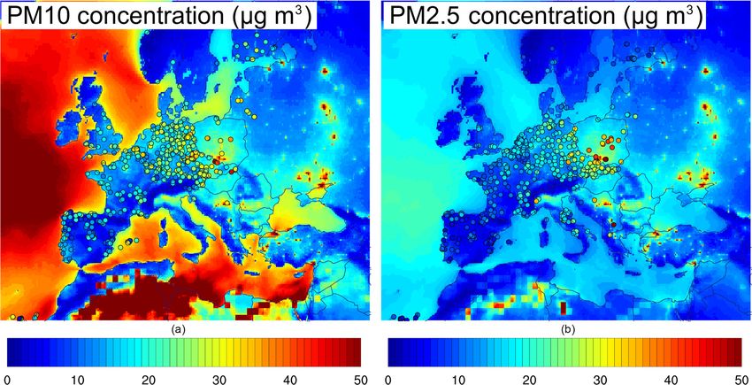
M. Descheemaecker et al.: Monitoring aerosols over Europe                                                                   1255

   While the observation operator is designed to assimilate       tion between the two data sets, the Spearman correlation is a
the AOD of any wavelength from the UV to the IR, the as-          mean used to assess their monotonic relationship.
similation system MOCAGE-PALM cannot assimilate data                 The AQeR stations are mainly located over western Eu-
on several wavelengths simultaneously (Sič et al., 2016).        rope (Fig. 2). After selection of the surface stations that are
This limitation is due to the choice of the control vector,       representative of background air pollution (following Joly
which is the 3-D total aerosol concentration: assimilating dif-   and Peuch, 2012), 597 and 535 stations are respectively used
ferent wavelengths simultaneously would require rethinking        for the PM10 –PM2.5 comparison. Figure 2 represents the
and extending the control vector, for instance splitting it by    mean surface concentration of the NR and selected AQeR
aerosol size bins or types. This explains why the study fo-       measurements over the domain from January to April 2014.
cuses on the assimilation of the AOD of a single wavelength.      The left panel shows the PM10 concentrations of the NR in
                                                                  the background and the AQeR concentrations as a circle,
2.4   Case study                                                  while the right panel shows the PM2.5 concentrations. The
                                                                  concentration of the NR PM10 and PM2.5 are generally un-
The period extends from 1 January to 30 April 2014 and in-        derestimated compared to the observations. Nevertheless, in
cludes several days of PM pollution over Europe. From 7           both figures, the spatial variability and, particularly, the lo-
to 15 March, a secondary-particle episode (EEA, 2014) oc-         cation of maxima are reasonably well represented. Over the
curs, while from 29 March to 5 April a dust plume originating     European continent, the NR and AQeR data show clear max-
from the Sahara propagates northwards to Europe (Vieno et         ima in the centre of Europe for both PM10 and PM2.5 con-
al., 2016).                                                       centrations, even if the NR underestimates these maxima.
   The MOCAGE simulation covers the whole period from                Table 1 shows the statistical indicators of this compari-
January to April 2014 on a global domain at 2◦ resolu-            son for hourly surface concentrations in PM10 and PM2.5 .
tion and in a nested regional domain, which covers Europe         A negative mean bias is observed, around −6.23 µg m−3
from 28 to 72◦ N and from 26◦ W to 46◦ E, at 0.2◦ reso-           (∼ −35.1 %) for PM10 and −3.20 µg m−3 (∼ −24.7 %) for
lution (see Fig. 2). A 4-month spin-up is made before the         PM2.5 . The RMSE is equal to 16.2 µg m−3 for PM10 and
simulation. The NR is forced by ARPEGE meteorological             11.9 µg m−3 for PM2.5 , while the FGE equals 0.56 and 0.543.
analysis. Emissions of chemical species in the global do-         The factor of 2 is equal to 64.7 % and 67.5 % for PM10 and
main come from the MACCity inventory (van der Werf et al.,        PM2.5 . Pearson and Spearman correlations are respectively
2006; Lamarque et al., 2010; Granier et al., 2011) for anthro-    0.452 and 0.535 for PM10 and PM2.5 and 0.537 and 0.602
pogenic gas species and biogenic species are from the Global      for PM10 and PM2.5 . The NR underestimation is greater for
Emissions InitiAtive (GEIA) for the global and regional do-       PM10 than for PM2.5 in relative differences. This suggests a
main. ACCMIP project emissions are used for anthropogenic         lack of aerosol concentrations in the PM10−2.5 (concentra-
organic and black carbon emissions on the global scale. The       tion of aerosols between 2.5 and 10 µm). Not taking into ac-
TNO-MACC-III inventory for the year 2011 provides anthro-         count wind-blown crustal aerosols may cause a potential un-
pogenic emissions in the regional domain. TNO-MACC-III            derestimation of PM in the models (Im et al., 2015). Taking
emissions are the latest update of the TNO-MACC inventory         them into account requires a detailed ground-type inventory
based on the methodology developed in the MACC-II project         to compute those emissions unavailable in MOCAGE. For
described in Kuenen et al. (2014). These anthropogenic emis-      PM2.5 , the underestimation of aerosol concentrations can be
sions are completed in our regional domain, at the boundary       due to a lack of carbonaceous species (Prank et al., 2016).
of the MACC-III inventory domain by emissions from MAC-           Other possible reasons for the negative PM bias at the sur-
City. Daily biomass burning sources of organic and black          face are the underestimation of emissions in the cold winter
carbon and gases from the Global Fire Assimilation Sys-           period and the uncertainty in the modelling of stable winter
tem (GFAS) (Kaiser et al., 2012) are injected in the model.       conditions with shallow surface layers.
The NR includes secondary organic aerosols (SOAs) in or-             A time-series graph of the median NR surface concen-
der to enhance its realism and to fit the observations made       trations and the median surface concentrations of the AQeR
at ground-based stations over Europe well. Standard ratios        stations are presented in Fig. 3. Compared to ground-based
from observations (Castro et al., 1999) are used to simulate      AQeR data (in black), the NR (in purple) generally under-
the portion of secondary carbon species, with 40 % in winter      estimates the PM10 and the PM2.5 concentrations, especially
from the primary carbon species in the emission input.            during the 7–15 March pollution episode. However, the vari-
   The NR is compared to the real observations from               ations and maxima of the NR concentrations of PM are gen-
AERONET AOD observations and AQeR surface concen-                 erally well represented. Furthermore, around 65 % of model
trations, using common statistical indicators: mean bias (B),     concentrations are relatively close to the observations as
modified normalized mean bias (MNMB), root mean square            shown by the factor of 2 in Table 1. The variability of NR
error (RMSE), fractional gross error (FGE), Pearson corre-        concentrations is thus consistent with AQeR station concen-
lation coefficient (Rp ) and Spearman correlation coefficient     trations.
(Rs ). While the Pearson correlation measures the linear rela-

www.atmos-meas-tech.net/12/1251/2019/                                               Atmos. Meas. Tech., 12, 1251–1275, 2019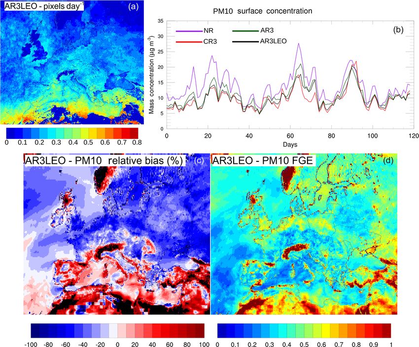
1256                                                                   M. Descheemaecker et al.: Monitoring aerosols over Europe

Figure 2. Mean PM10 (a) and PM2.5 (b) surface concentration (µg m−3 ) of the NR (shadings) and AQeR stations (colour circles) from
January to April 2014.

Table 1. Bias, RMSE, FGE, factor of 2, Pearson correlation (Rp ) and Spearman correlation (Rs ) of the NR simulation taking as reference
the AQeR observations for hourly PM10 and PM2.5 concentrations from January to April 2014.

                                     Bias (µg m−3 )         RMSE (µg m−3 )           FGE      FactOf2       Rp       Rs
                       NR PM10       −6.23                            16.2            0.56      64.7 %    0.452    0.537
                                     (∼ −35.1 %)
                       NR PM2.5                                       11.9           0.543      67.5 %    0.535    0.602
                                     −3.20 (∼ −24.7 %)

   Table 2 gives an evaluation of the NR against the daily                   Table 2. Bias, MNMB, RMSE, FGE and Pearson correlation (Rp )
mean of the AOD at 500 nm obtained from 84 AERONET                           between the NR simulation and AERONET station for daily 500 nm
stations in the regional domain from January to April 2014.                  AOD from January to April 2014.
The statistical indicators show good consistency between the
NR and AERONET observations. However, like the results                                        Bias   MNMB         RMSE     FGE      Rp
shown on a global scale (Sič et al., 2015), MOCAGE tends to                        NR       0.043       0.39      0.09    0.531   0.56
overestimate AOD: although small, the AOD bias is positive.
While PM concentrations at the surface are underestimated in
the NR, there may be different reasons for an overestimation
of AOD. The vertical distribution of aerosol concentrations                  derestimating PM at the surface. However, both the PM and
in the model is largely controlled by vertical transport, re-                AOD correlation errors of the NR remain in a realistic range.
moval processes and by the prior assumptions on the aerosol                     As a result, the NR simulation exhibits surface concentra-
emission profiles. However, these processes may have large                   tions and AODs in the same range compared to those from
variability and they are prone to large uncertainties (Sič et al.,          ground-based stations and shows similar spatial and temporal
2015). Another possible explanation is the uncertainty of the                variations, which makes the NR acceptable for the OSSE.
size distribution of aerosols that can significantly affect the
optical properties. More generally, the assumptions that un-
derly the computation of optical properties are largely uncer-               3   Generation of synthetic AOD observations
tain and they can affect the computation of AOD by a factor
of 50 % (Curci et al., 2015): the mixing state assumption, and               The study focuses on the added value of assimilating AODs
the uncertainty in refractive indices and in hygroscopicity                  at the central wavelength (444 nm) of the FCI/VIS04 spec-
growth. These uncertainties in aerosol vertical profiles, size               tral band. Since the assimilation of AODs from several wave-
distribution and optical properties may explain the decorrela-               lengths simultaneously is not possible (Sect. 2.3), the choice
tion between AOD and PM concentrations at the surface and                    of the single-channel VIS04 is mainly driven by the fact that
why the MOCAGE NR has a positive bias in AOD while un-                       it is the shortest wavelength of FCI, which is a priori the most
                                                                             favourable for the detection of fine particles.

Atmos. Meas. Tech., 12, 1251–1275, 2019                                                         www.atmos-meas-tech.net/12/1251/2019/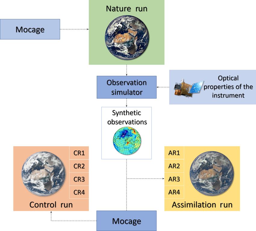
M. Descheemaecker et al.: Monitoring aerosols over Europe                                                                               1257

Figure 3. Median of the daily mean surface concentration in µg m−3 of the NR (in purple) and the AQeR station (in black). The NR
concentrations are calculated at the same locations as the AQeR stations from 1 January 2014 (Day 1) to 30 April 2014 (last day). The left
panel is for PM10 surface concentrations, while the right one is for PM2.5 .

   Thus, synthetic AOD observations at 444 nm are created
over the MOCAGE-simulated regional domain from the NR
simulation 3-D fields: all aerosol concentrations per type and
per size bins, and meteorological variables. At every grid
point of the NR regional domain where the solar zenith an-
gle is below 80◦ (daytime) and where clouds are absent, an
AOD value at 444 nm is computed using the MOCAGE ob-
servation operator described above (Sect. 2.3). In order to
take into account the error characteristics of the FCI VIS04
AOD, a random noise is then added to this NR AOD value.
   To estimate the variance of this random noise, the general
principle is to assess and quantify the respective sensitivity
of the FCI VIS04 top-of-the-atmosphere reflectance to AOD
and to the other variables. To do this, the FCI simulator de-
veloped by Aoun et al. (2016), based on the radiative trans-
fer model (RTM) libRadtran (Mayer and Killings, 2005), has             Figure 4. Classification of the NR profiles for the 7 March 2014
been used. This simulator computes the reflectance in the dif-         at 12:00 UTC. Deep blue is for dismissed profiles, blue is for mar-
ferent spectral bands of FCI as a function of different input          itime clean, light blue for maritime polluted, green is for continental
atmospheric parameters (AOD τ , total column water vapour,             clean, yellow is for continental 5 average, orange is for continental
ozone content), ground albedo ρg and solar zenith angle θS ,           polluted, deep orange is for urban, and red is for desert dust.
for different OPAC (optical properties of aerosols and clouds,
Hess et al., 1998) aerosol types: dust, maritime clean, mar-
itime polluted, continental clean, continental average, conti-
                                                                       and [DD] > [IWS]. An example of NR profiles (7 March 2014
nental polluted and urban. The FCI simulator takes into ac-
                                                                       at 12:00 UTC) decomposed in OPAC type is presented in
count the spectral response sensitivity and the measurement
                                                                       Fig. 4. A small number of the profiles are dismissed where
noise representative of the FCI VIS04 spectral band (415–
                                                                       MOCAGE profiles do not match one of the OPAC types, such
475 nm).
                                                                       as profiles over ocean where IWS (insoluble, water soluble
   By applying a global sensitivity analysis to this FCI sim-
                                                                       and soot; Table 3) is greater than DD (desert dust) and SS
ulator that was run on a large data set (see the Appendix
                                                                       (sea salt). A larger number of profiles are dismissed because
for the details of the method), a look-up table of the RMSE
                                                                       of night-time profiles and cloudy conditions. Figure 5 repre-
of AOD is derived. It depends on the OPAC type, the rela-
                                                                       sents the average number of NR AODs that are retained per
tive error of surface albedo, the solar zenith angle and the
                                                                       day for assimilation. After these filters apply, between 10 %
ground albedo value. The classification of each MOCAGE
                                                                       and 20 % of profiles are kept every hour. The density of these
profile into the OPAC types relies on three parameters (Ta-
                                                                       profiles is higher in the south of the domain, which is directly
ble 3): the surface concentration, the main surface species
                                                                       correlated to the quantity of direct sunlight available. Over
and the proportion in relation to the total aerosol concentra-
                                                                       the continent, between 1 and 4 profiles can be assimilated
tions. A species is described as a main species if its concen-
                                                                       per day at each grid-box location.
tration, [species], is above the concentration of all other types
                                                                          On every NR profiles that is kept, an AOD error is in-
of aerosol. For example DD is a main species if [DD] > [SS]
                                                                       troduced, by addition of a random value from an unbiased

www.atmos-meas-tech.net/12/1251/2019/                                                      Atmos. Meas. Tech., 12, 1251–1275, 2019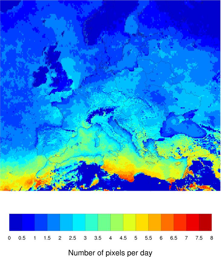
1258                                                                    M. Descheemaecker et al.: Monitoring aerosols over Europe

Table 3. Conditions for classifying the MOCAGE NR into the OPAC types. The first condition is the surface concentrations, the second is the
main specie at the surface between desert dust (DD), sea salt (SS) and IWS (insoluble, water soluble and soot) and the third is a condition of
the species over all the aerosol concentrations. A species is described as a main species if its concentrations is above all other concentrations;
for example DD is a main species if [DD] > [SS] and [DD] > [IWS].

                                Aerosol types            Surface      Main species            Surface proportion
                                                 concentration in     over the total PM10
                                                         µg m−3
                                DO. and DC.                      –    DD
                                MC.                              –    SS                      SS > 85 %
                                MPO.                             –    SS                      SS < 85 %
                                MPC.                             –    SS                      SS < 85 %
                                CC.                          0–17     IWS
                                CA.                         17–34     IWS
                                CP.                         34–75     IWS
                                U.                            > 75    IWS

                                                                            4   Controls runs (CRs) and their comparison to NR

                                                                            Section 2 showed an evaluation of the NR compared to real
                                                                            observations. Another requirement of the OSSE is the evalu-
                                                                            ation of differences between the NR and the CR. Various CR
                                                                            simulations have been performed to evaluate the behaviour of
                                                                            the OSSE in different CR configurations and prove its robust-
                                                                            ness. The NR and CRs use different set-ups of MOCAGE.
                                                                            The CRs use IFS meteorological forcings, while the NR uses
                                                                            ARPEGE meteorological forcings. The use of different mete-
                                                                            orological inputs is expected to yield differences in the trans-
                                                                            port of pollutant species, and changes in dynamic emissions
                                                                            of sea salt and desert dust. To introduce more differences be-
                                                                            tween the CRs and NR, changes in the emissions are also
                                                                            introduced.
                                                                               Table 4 indicates the changes made to the different model
                                                                            parameters to create four distinct CR simulations. The first
                                                                            control run, CR1, uses the same inputs as the NR except for
                                                                            the meteorological forcings. Other control runs (CR2, CR3,
                                                                            CR4) do not have the SOA formation process of the NR
Figure 5. Average (from January to April) number of selected pro-           (Sect. 2) and CR1 simulations. Finally, CR3 and CR4 change
files per day available for assimilation.                                   from other simulations by different vertical repartitions of
                                                                            emissions in the five lowest levels. In CR3, the pollutants are
                                                                            emitted with a slower decay with height than the NR (with
Gaussian with a standard deviation derived from the AOD                     repartition from 30 % at the surface and respectively 24 %;
RMSE look-up table, calculated as explained above. The sur-                 19 %; 15 %; 12 % for the four levels above), and in the CR4
face albedo fields are taken from MODIS using the radiative                 emissions are only injected in the lowest level. These changes
transfer model RTTOV (Vidot et al., 2014). A relative error                 aim to generate simulations that are more significantly differ-
of 10 % is assumed for ground albedo, which corresponds to                  ent from the NR than the first two control runs.
a realistic value (Vidot et al., 2014). An example of the syn-                 The four CRs are compared to the NR for PM10 and PM2.5
thetic observations is presented in Fig. 6. It represents the NR            surface concentration considering virtual observations at the
AOD, the synthetic observations and the noise applied to NR                 same locations as the AQeR stations. A time series of daily
AOD for the 7 March 2014 at 12:00 UTC.                                      means of surface concentrations at simulated stations is pre-
                                                                            sented in Fig. 7 for NR and CR simulations from 1 January to
                                                                            30 April 2014. The PM10 concentrations of the NR (in pur-
                                                                            ple) are mostly greater than the PM10 concentrations in the
                                                                            CRs. During the period of late March and early April (around

Atmos. Meas. Tech., 12, 1251–1275, 2019                                                         www.atmos-meas-tech.net/12/1251/2019/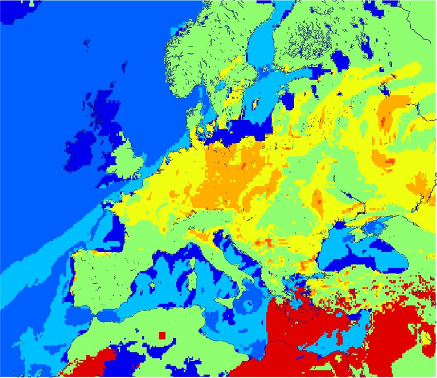
M. Descheemaecker et al.: Monitoring aerosols over Europe                                                                                 1259

Figure 6. Example of generation of synthetic observations on the 7 March 2014 at 12:00 UTC. From the NR AOD as 444 nm (a), noise
values representative of FCI (b) are applied to every clear-sky pixel to generate the synthetic observations (c). The grey colour represents the
dismissed profiles.

Table 4. Table of differences between the NR simulation and the           around −2.9 µg m−3 (−20.5 %) for PM10 and −1.8 µg m−3
CR simulations.                                                           (−15.1 %) for PM2.5 . The two other CRs highly under-
                                                                          estimate PM10 and PM2.5 concentrations with biases of
            Forecasts    SOA      Repartition of emissions                −4.5 µg m−3 (−35.2 %) and −3.9 µg m−3 (−37.4 %) respec-
                                  from level 1 (surface layer)            tively for CR2 and −4.8 µg m−3 (−38.1 %) and −4.4 µg m−3
                                  up to the fifth level
                                                                          (−42.6 %) for the CR3. These biases are in agreement with
   NR       ARPEGE       Yes      52 %; 26 %; 13 %; 6 %; 3 %              the literature. Prank et al. (2016) measure a bias around −5.8
   CR1      IFS          Yes      52 %; 26 %; 13 %; 6 %; 3 %              for PM10 and −4.4 µg m−3 for PM2.5 for the median of four
   CR2      IFS          No       52 %; 26 %; 13 %; 6 %; 3 %              CTMs against ground-based stations in winter. In Marécal
   CR3      IFS          No       30 %; 24 %; 19 %; 15 %; 12 %            et al. (2015), statistical indicators for an ensemble of seven
   CR4      IFS          No       100 %; 0 %; 0 %; 0 %; 0 %               models are presented for winter. A bias between −3 and
                                                                          −7 µg m−3 is observed for the median ensemble. The PM
                                                                          concentrations of our CRs compared to the NR are charac-
                                                                          teristic of models compared to observations.
the 90th day of simulation) the NR concentrations of PM10
                                                                             Prank et al. (2016) also show other indicators of the me-
are close to those of the CR2, CR3 and CR4, and less than
                                                                          dian of models, such as the temporal correlation and the fac-
those of the CR1 by about a few µg m−3 . In terms of PM2.5 ,
                                                                          tor of 2. Their correlations are around 0.7 for PM2.5 and
the CR concentrations also underestimate the NR concentra-
                                                                          0.6 for PM10 and are close to those for our CR simulations
tion. As for PM10 , around the 90th day of simulation, the
                                                                          that vary from 0.644 to 0.732 for PM2.5 and from 0.572 to
concentrations of CR1 are above the concentrations of the
                                                                          0.671 for PM10 . Their factor of 2 equals 65 % for PM10 and
NR.
                                                                          67 % for PM2.5 . The factor of 2 of the CRs ranges between
   These tendencies can also be observed in Fig. 8, which
                                                                          70 % and 90 % for both PM10 and PM2.5 concentrations. The
represents a scatter plot of CR concentrations as a function of
                                                                          RMSE of CR simulations ranges from 8 to 10 µg m−3 for
NR concentrations for the daily means of surface concentra-
                                                                          PM10 concentrations, which is slightly under the RMSE of
tion in PM10 and PM2.5 at the virtual stations. The CR1 con-
                                                                          the ensemble from the study of Marécal et al. (2015), which
centrations are fairly close to those of the NR concentrations
                                                                          ranges between 10 and 15 µg m−3 . The FGE of the study of
with a coefficient of regression about 0.801 and 0.835 for
                                                                          Marécal et al. is equal to 0.55, while the FGE of CRs varies
PM10 and PM2.5 . Other CRs underestimate the NR concen-
                                                                          from 0.33 to 0.51. Our CR simulations slightly underestimate
trations. This tendency is stronger for PM10 than for PM2.5 .
                                                                          the model relative error. Thus, compared to the literature, the
The regression coefficients of the CR2, CR3 and CR4 are re-
                                                                          CRs (especially the CR3) are different enough from the NR
spectively 0.596, 0.583 and 0.607 for PM10 and 0.570, 0.505
                                                                          to be representative of state-of-the-art simulations.
and 0.647 for PM2.5 . For both PM10 and PM2.5 concentra-
                                                                             Between the CRs and the NR there are important spatial
tions, the underestimation is more important for high values
                                                                          differences in the surface concentrations of PM, as demon-
of the NR concentrations than for low values.
                                                                          strated in Fig. 9, which shows the relative differences, Pear-
   The statistical indicators in Tables 5 and 6 are con-
                                                                          son correlation and the FGE for PM10 . Over the Atlantic
sistent with Figs. 7 and 8. The CR1 is close to the
                                                                          Ocean, the CR concentrations are relatively close to the NR,
NR with a bias of −1.3 µg m−3 (−8.2 %) for PM10
                                                                          except for the CR4 which overestimates the concentration of
and −0.8 µg m−3 (−6.2 %) for PM2.5 . The CR4 bias is

www.atmos-meas-tech.net/12/1251/2019/                                                         Atmos. Meas. Tech., 12, 1251–1275, 2019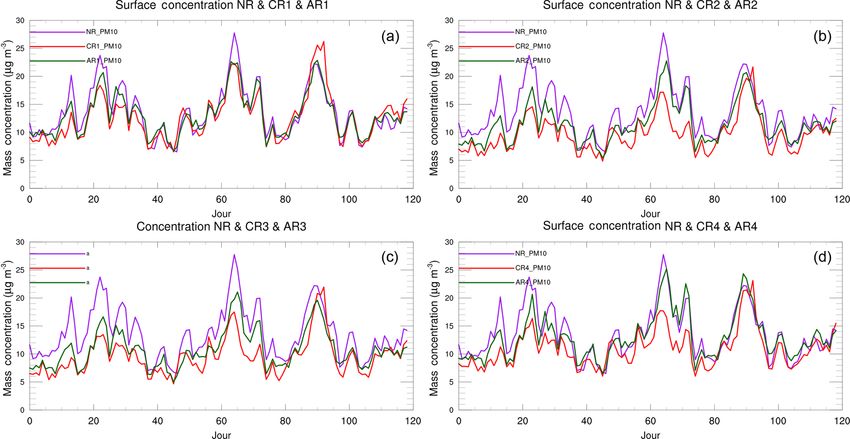
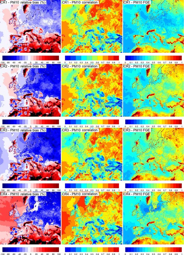
1260                                                               M. Descheemaecker et al.: Monitoring aerosols over Europe

Figure 7. Median of the daily mean surface concentration of the NR (in purple) and the different CRs (CR1 in green, CR2 in yellow, CR3 in
red and CR4 in blue) determined for the same location as for the AQeR stations. Panel (a) is the PM10 mass concentration (µg m−3 ), while
(b) represents the PM2.5 mass concentrations.

Figure 8. Scatter plot of the CR daily surface concentrations (µg m−3 ) as a function of NR daily surface concentrations for PM10 (a) and
PM2.5 (b), for virtual stations and from January to April 2014. rgCRX are the linear regressions of each data set.

PM10 . All CRs present high concentrations of PM10 all over            east axis. The correlations are slightly greater for CR1 than
northern Africa. This corresponds to high emissions of desert          for the other CRs. The FGE over the continent changes sig-
dust over this area, which cause an important overestimation           nificantly for CR1 and the other CRs, respectively around
of PM10 compared to the NR. This overestimation can be ob-             0.35 and 0.55. Similar conclusions can be obtained for the
served around all the Mediterranean Basin. The CRs tend to             PM2.5 comparison (see Supplement). A similar comparison
overestimate the PM10 concentrations over Spain, Italy, the            has been done for the AOD between the CR simulations and
Alps, Greece, Turkey, the north of the UK, Iceland and Nor-            the NR simulation (see complementary materials).
way. The overestimations over the Alps, Iceland and Norway                In summary, the control runs present spatial variability
are located at places of negligible concentrations. Over the           along with temporal variability. The closest CR to the NR
rest of the European continent, CRs underestimate the con-             is the CR1. In terms of surface concentrations in PM, the
centration of PM10 , slightly for CR1, but concentrations are          CR3 is the most distant, while in terms of AOD the CR4 is
very pronounced for CR2, CR3 and CR4. The area where the               the most distant. Those differences and the use of different
consistency between the CRs and the NR is better is the At-            CRs, coupled with the realism of the NR, demonstrate the
lantic Ocean, with a correlation ranging from 0.6 to 0.9 and           robustness of the OSSE to evaluate the added value provided
a low FGE around 0.3. Over the Mediterranean Basin the                 by AOD derived from the FCI.
correlation varies significantly between 0 and 1. Low cor-
relations correspond to high FGE around 1. Over the conti-
nent, the correlation varies from 0.4 to 0.9, following a west–

Atmos. Meas. Tech., 12, 1251–1275, 2019                                                   www.atmos-meas-tech.net/12/1251/2019/
M. Descheemaecker et al.: Monitoring aerosols over Europe                                                                          1261

Table 5. Bias, RMSE, FGE, factor of 2, Pearson correlation (Rp ) and Spearman correlation (Rs ) of the CR simulation taking as reference
the NR simulations for hourly PM10 concentrations from January to April 2014. The comparison is made at the same station location as for
AQeR stations.

                 Hourly PM10 CR stations      Bias (µg m−3 )     RMSE (µg m−3 )      FGE     FactOf2       Rp       Rs
                 vs. NR stations
                 CR1                          −1.3 (−8.2 %)             7.9          0.332     89.1 %    0.671   0.748
                 CR2                          −4.5 (−35.2 %)            9.3           0.47     75.6 %    0.609   0.709
                 CR3                          −4.8 (−38.1 %)            9.8          0.511     69.3 %    0.572   0.671
                 CR4                          −2.9 (−20.5 %)            8.7          0.412     81.9 %    0.623   0.712

Table 6. Bias, RMSE, FGE, factor of 2, Pearson correlation (Rp ) and Spearman correlation (Rs ) of the CR simulation taking as reference
the NR simulations for hourly PM2.5 concentrations from January to April 2014. The comparison is made at the same station location as for
AQeR stations.

                 Hourly PM2.5 CR stations      Bias (µg m−3 )    RMSE (µg m−3 )       FGE     FactOf2      Rp       Rs
                 vs. NR stations
                 CR1                          −0.8 (−6.24 %)            5.9          0.307     91.1 %    0.732    0.776
                 CR2                          −3.9 (−37.4 %)            7.1          0.452     78.4 %     0.69    0.731
                 CR3                          −4.4 (−42.6 %)            7.6          0.505     70.6 %    0.644    0.695
                 CR4                          −1.8 (−15.1 %)            6.6          0.374     85.5 %    0.665     0.73

5   Assimilation of FCI synthetic observations                         lation on the simulation while not having multiple coverage
                                                                       of assimilated observations over one profile. The result of
The purpose of this paper is to assess the potential contribu-         this thinning procedure changes the assimilated fields only
tion of the FCI VIS04 channel to the assimilation of aerosols          slightly but significantly saves computing time. Assimilation
on a continental scale. In our OSSE, MOCAGE represents                 simulations (ARs) are run for all CR simulations using the
the atmosphere with a horizontal resolution of 0.2◦ (around            same generated set of synthetic observations over the period
20 km at the equator). Synthetic observations are therefore            of 4 months, from 1 January to 30 April. The standard de-
computed at the model resolution, although FCI scans around            viation of errors used for B and R matrices are estimated
1 km resolution at the equator and 2 km over Europe. To                respectively at 24 % and 12 %, as in Sič et al. (2016).
fit with the time step of our assimilation cycle, synthetic               To assess the impact of the assimilation of FCI synthetic
observations are also created every hour, although the fu-             AOD observations, the CR forecasts and the AR analyses
ture FCI imager could retrieve radiance observations every             are compared to the assimilated synthetic observations. Fig-
10 min over the globe, and 2.5 min over Europe with the Eu-            ure 10 shows the histograms of the differences between the
ropean Regional-Rapid-Scan. This means that, for each pro-             synthetic observations and the forecast field (in blue) and
file of our simulation, only one synthetic observation is avail-       between synthetic observations and analysed fields (in pur-
able each hour, instead of 24 × 10 × 10 at best (FCI scans 24          ple) for the four ARs simulations. The histograms follow a
times an hour, with a spatial resolution 10 times higher than          Gaussian shape, and the distribution of the analysed values
the model over the Europe). The use of one observation for             are closer to the synthetic observations than the forecast val-
each profile in an assimilation window is due to the assim-            ues. The spread of the histograms is smaller for the anal-
ilation system design that does not allow multiple observa-            ysed fields than for the forecast fields. The assimilation of
tions for the same profile. In practice, future FCI observations       synthetic AODs hence improved the representation of AOD
could be averaged over each MOCAGE profile to reduce the               fields in the assimilation simulations. Besides, the spatial
impact of the instrument errors on assimilated observations.           comparisons between the simulations and the NR show im-
   The 3D-FGAT assimilation scheme integrates the syn-                 provements in the AOD fields of simulations by assimilation
thetic observations described in Sect. 3. Before assimilation,         of the synthetic observations (see Supplement Figs. S5, S6,
a thinning process is applied to the synthetic observations to         S7 and S8). As the increment is applied to all aerosol bins
spatially keep only 1 pixel out of 4. Such thinning is use-            and PM10 corresponds to 5 of the 6 bins while PM2.5 to only
ful for reducing the computation time, by accelerating the             4, we expect better corrections for PM10 concentrations than
convergence of the cost function (not shown). The spatial              for PM2.5 concentrations.
correlation length of the B background covariance matrix is               To validate the results of the OSSEs, the simulations are
set to 0.4◦ in order to have a spatial impact of the assimi-           compared to the reference simulation (NR) over the period.

www.atmos-meas-tech.net/12/1251/2019/                                                    Atmos. Meas. Tech., 12, 1251–1275, 2019
1262 M. Descheemaecker et al.: Monitoring aerosols over Europe
Table 7. Bias, RMSE, FGE, factor of 2, Pearson correlation and Spearman correlation of the ARs simulation taking as reference the NR
simulations for hourly PM10 concentrations from January to April 2014. The comparison is made at the same station location as for AQeR
stations.
Hourly PM10 CR stations Bias (µg m−3 ) RMSE (µg m−3 ) FGE FactOf2 Rp Rs
vs. NR stations
AR1 −1.17 (−7.21 %) 7.16 0.296 92.2 % 0.739 0.791
AR2 −2.91 (−21.3 %) 8.1 0.373 85.3 % 0.694 0.751
AR3 −3.53 (−26.2 %) 8.67 0.417 80.4 % 0.67 0.726
AR4 −0.756 (−5.31 %) 8.03 0.339 88.2 % 0.691 0.759
Figure 11 exhibits the spatial differences in the surface con- concentrations than for the PM2.5 concentrations, which was
centrations of PM10 between the ARs and the NR. It shows expected.
the mean relative bias, the correlation and the FGE for every In AR4, the PM10 bias over the Atlantic Ocean is posi-
simulation. Using Fig. 9 as a reference, the relative bias, the tive and larger than in CR4: the assimilation of FCI AODs
FGE and the correlation have been improved over most parts can be detrimental in some circumstances. A reason for such
of the domain after assimilation for all simulations. Over deficiencies is proposed. In CR4, the AOD bias is negative
the European continent, all simulations show a strong im- (see Supplement) but the PM10 bias is positive (Fig. 9) due
provement of the statistical indicators. For instance in CR3, to a vertical distribution of emissions limited to the lowest
along a line that goes from Spain to Poland, the FGE de- MOCAGE level. As a result of the assimilation, the aerosol
creases by about 0.1 after assimilation. In the eastern part increments associated with the synthetic AOD observations
of Europe (from Turkey to Finland), the decrease in FGE are positive and they are responsible for increasing the PM10
is even higher. Over northern Africa and the Mediterranean fields at the surface. In the other CRs, the AOD bias over the
Sea the improvement is intermediate. Nevertheless, the mean Atlantic is mostly negative, as the PM bias, and the ARs are
bias over the ocean tends to increase for the simulations, es- better than the corresponding CRs. In other words, where the
pecially for AR4. This can also be observed for the PM2.5 surface PM bias and the AOD bias do not have the same sign,
concentration comparison (see Figs. S1, S2, S3 and S4). the assimilation of AODs can be detrimental.
The assimilation of the synthetic observations has a pos- To evaluate the capability of the FCI 444 nm channel ob-
itive impact at each layer of the model. The mean vertical servations to improve aerosol forecast in an air quality sce-
concentrations of PM10 and PM2.5 of the different simula- nario, the AR simulations have been compared to the NR us-
tions are represented in Figs. 12 and 13, from the surface ing the synthetic AQeR stations as in Sect. 4. Tables 7 and 8
(level 47) up to 6 km (level 30). The positive impact along the show the statistics of the comparison between the ARs and
vertical of the assimilation of AODs in the CTM MOCAGE the NR for PM10 and PM2.5 concentrations. With regard to
is due to the use of the vertical representation of the model the comparison of the CRs against the NR in Tables 5 and 6,
to distribute the increment. Sič et al. (2016) showed that the the ARs are more consistent with the NR. The bias is reduced
assumption of using the vertical representation of the model for both PM10 and PM2.5 concentrations. The RMSE and the
gives good assimilation results with the regular MOCAGE FGE decrease, while the factor of 2 and the correlations in-
set-up, which distributes emissions over the five lowest verti- crease for all ARs compared to their respective CRs.
cal levels. However, the performance of the assimilation may The daily medians of PM10 and PM2.5 concentrations at all
depend on the realism of the representation of aerosols along stations are represented over time in Figs. 14 and 15 for the
the vertical in the CTM. The CR simulations, in red, overesti- four simulations. The assimilation reduces the gap between
mate the PM10 concentrations of the NR, in purple, due to the the simulations and the NR over the entire period. Around the
overestimation of desert dust concentrations in the CR simu- secondary inorganic aerosol episode, on the 65th day of sim-
lations. This overestimation is not present in the PM2.5 con- ulation, the improvements of PM10 and PM2.5 surface con-
centrations because this is the fraction of aerosols in which centrations are significant for simulations 2, 3 and 4.
there is little desert dust. For the first three simulations, the From an air quality monitoring perspective, the assimi-
vertical PM10 concentrations are corrected well by the as- lation of the FCI synthetic AOD at 444 nm in MOCAGE
similation, while for simulation 4, the correction is less rel- improves strongly the surface PM10 concentrations in the
evant for the levels near the surface. The assimilation tends four simulations over the European continent for the period
to decrease the PM2.5 concentrations above level 42 and to January–April 2014.
increase the concentrations under that level. Simulation 4 To quantify the improvement in simulations through the
presents a decay of the surface concentrations of PM2.5 . The assimilation of FCI synthetic observations during a severe-
correction of concentrations is more pertinent for the PM10 pollution episode for (7–15 March) over Europe, maps of rel-
Atmos. Meas. Tech., 12, 1251–1275, 2019 www.atmos-meas-tech.net/12/1251/2019/M. Descheemaecker et al.: Monitoring aerosols over Europe 1263 Figure 9. For each CR (CR1, CR2, CR3 and CR4), the figures represent a PM10 comparison between the NR and the CRs from January to April 2014: the relative bias (in %), the Pearson correlation and the fractional gross error. ative concentrations of PM10 and FGE are respectively rep- the continent in the simulations, but the simulations still un- resented for the CR comparison and for the AR comparison derestimate the PM10 concentrations by 30 %–20 %. Impor- in Figs. 16 and 17. The simulations CR2, CR3 and CR4 un- tant changes in the FGE are noticeable, with values dropping derestimate PM10 concentrations for 70 % over all Europe from 0.55–0.85 down to 0.2–0.4 for all simulations. Over the compared to the NR. The FGE presents high values from other areas, the assimilation significantly reduces the relative 0.55 to 0.85. The assimilation of synthetic AOD meaning- bias and the FGE. Thus, the assimilation of synthetic obser- fully improves the surface concentrations of aerosols over vations significantly improves the representation of the sur- www.atmos-meas-tech.net/12/1251/2019/ Atmos. Meas. Tech., 12, 1251–1275, 2019
1264                                                                   M. Descheemaecker et al.: Monitoring aerosols over Europe

Table 8. Bias, RMSE, FGE, factor of 2, Pearson correlation and Spearman correlation of the ARs simulation taking as reference the NR
simulations for hourly PM2.5 concentrations from January to April 2014. The comparison is made at the same station location as for AQeR
stations.

               Hourly PM2.5 ARs stations      Bias (µg m−3 )           RMSE (µg m−3 )       FGE    FactOf2      Rp        Rs
               vs. NR stations
               AR1                            −0.395 (−3.15 %)                5.61       0.284      92.7 %    0.755    0.806
               AR2                            −2.28 (−20.5 %)                 6.31       0.364      86.6 %    0.703    0.766
               AR3                            −2.94 (−27.1 %)                 6.86       0.416      80.9 %    0.669    0.732
               AR4                            0.109 (0.9 %)                   6.56       0.328      89.4 %    0.699    0.765

Table 9. Bias, RMSE, FGE, factor of 2, Pearson correlation and Spearman correlation of the AR3LEO simulation taking as reference the NR
simulations for hourly PM10 and PM2.5 concentrations from January to April 2014. The comparison is made at the same station location as
for AQeR stations.

                 Hourly AR3LEO stations       Bias (µg m−3 )          RMSE (µg m−3 )    FGE       FactOf2      RP       RS
                 vs. NR stations
                 PM10                         −4.47 (−35.1 %)              9.11         0.462      75.6 %    0.656    0.717
                 PM2.5                        −3.89 (−37 %)                7.14         0.457      76.5 %    0.681    0.731

                                                                          the European continent and the Mediterranean area. The im-
                                                                          provement of the vertical profile of aerosol concentrations is
                                                                          also noticeable, and it may be explained because different
                                                                          parts of the column can be transported by winds in differ-
                                                                          ent directions (Sič et al., 2016), although the synthetic AOD
                                                                          observations do not provide information along the vertical.
                                                                          The first two simulations give better results over the ocean
                                                                          than simulations 3 and 4 due to a closer representation of the
                                                                          vertical profile of the aerosol concentrations. This may show
                                                                          an overly optimistic aspect of the OSSE of the first two sim-
                                                                          ulations. The simulations lead to sufficiently reliable results
                                                                          since the shapes of their vertical profile of aerosol concentra-
                                                                          tions are different from those of the NR. These differences
                                                                          are caused by the way emissions are injected in the atmo-
                                                                          sphere (higher for simulation 3 and lower for simulation 4).
                                                                          The simulations 3 and 4 present robust results over the conti-
                                                                          nent, despite the differences in the vertical representation of
                                                                          aerosol concentrations.

                                                                          6    Discussion
Figure 10. Histograms of differences between synthetic observa-
tions and forecast fields (blue) and between synthetic observations
                                                                          Although the results have shown a general benefit of
and analysed fields (purple) for the four assimilation runs.
                                                                          FCI/VIS04 future measurements for assimilation in the CTM
                                                                          MOCAGE, some limitations must be addressed. The AOD
                                                                          does not introduce information on the vertical distribution of
face PM10 concentrations of simulations during the pollution              PM, nor on the size distribution and type of aerosols. So, the
episode.                                                                  performance of the assimilation will largely depend on the
   In summary, the use of synthetic observations at 444 nm                realism of the representation of aerosols in the CTM before
of the future sensor FCI through assimilation significantly               assimilation. If, for instance, the model has a positive bias
improves the aerosol fields of the simulations over the Eu-               in AOD and a negative bias in surface PM10 compared to
ropean domain from January to April 2014. These improve-                  observations, then the assimilation could lead to detrimental
ments are located all over the domain with best results over              results. So the AOD and PM biases should be assessed and

Atmos. Meas. Tech., 12, 1251–1275, 2019                                                      www.atmos-meas-tech.net/12/1251/2019/
You can also read