Romeo and Juliet in Brazil: Use of Metaphorical Models for Feedback Systems Thinking
←
→
Page content transcription
If your browser does not render page correctly, please read the page content below

Romeo and Juliet in Brazil:
Use of Metaphorical Models for
Feedback Systems Thinking

This paper is a contributing chapter to the book, Tracing Connections: Voices of
Systems Thinkers. In tribute to Barry Richmond, a leader and pioneer thinker
in system dynamics, the book shares stories about systems thinking and the
importance of its use in a world of growing interdependence.

reproduced in any form by any means without explicit permission in
writing from the publishers.

STELLA® and          ® are registered trademarks of isee systems, inc.

isee systems, inc.
31 Old Etna Rd Suite 7N                      27 Central Street
Lebanon NH 03766
603-448-4990 | www.iseesystems.com           978-635-9797 | www.clexchange.org
6
Romeo and Juliet in Brazil:
Use of Metaphorical Models for
Feedback Systems Thinking
John Morecroft
T
he attention and imagination of our
John Morecroft shares
his story of systems group of system dynamics doctoral
thinking consulting work students was captured during our
done with MBA students. years together by a working paper written
He discusses the spectrum by Nathaniel Mass and Peter Senge, “Under
of models—from fisheries standing Oscillations in Simple Systems.”
to “Romeo and Juliet” to I still recommend the paper today.1 The fol
global oil production—that
lowing excerpt reveals the authors’ intention
he used to illustrate some
of the conceptual skills of
to explain dynamics clearly and rigorously in
the modeler and feedback plain English by interpreting simulations:
systems thinker.
Acquiring a firm intuitive understanding of the
possible types of behavior produced by simple
first, second and third-order systems marks an important step in learning system
dynamics. Such simple systems frequently embody generic structures that recur in
a wide variety of complex systems. However, an intuitive grasp of simple oscillat-
ing systems often eludes both the beginning student and practitioner alike. Even
individuals familiar with the mathematics of dynamic feedback systems often
cannot provide a simple non-technical explanation of why a continuous first-order
system cannot possibly oscillate, or why a second-order system can. For example,
overshoot or oscillation in a system is often explained to result from “system
delays” or “inertia.” Vague explanations such as these impart little understanding of
how decisions being made in a system generate observed problems and behavior.
This paper presents some arguments we have used in past introductory courses
in system dynamics to successfully develop insight into simple oscillating systems.
9596 John Morecroft
The paper analyses a one-level model for
John Morecroft is Senior Fellow
in Management Science and the population growth of rabbits in a closed
Operations at London Business field to illustrate why a first-order negative
School where he teaches system feedback system exhibits a smooth transi-
dynamics, problem structuring tion to equilibrium instead of overshoot or
and strategy in MBA, Ph.D., and
oscillating behavior. The paper also analyzes
Executive Education programs.
He has served as Associate a simple inventory-workforce model to pro-
Dean of the School’s Executive vide an intuitive explanation of the causes
MBA programs and co-designed of convergent, divergent, and undamped
EMBA-Global, a dual degree oscillations.2
program with New York’s
Columbia Business School.
Morecroft is a leading expert in
strategic modeling and system
dynamics and has written more Communicating Feedback Systems
than fifty papers and journal
articles. Thinking in a Management
He has co-edited three books, Environment: The Braskem Course
written a system dynamics text
book, Strategic Modeling and
Business Dynamics (Wiley 2007), The dynamic insights we uncovered long ago in
and he is a recipient of the Jay MIT’s building E40 remain vivid and relevant
Wright Forrester Award of the today—as I discovered in October 2007. I lec
System Dynamics Society and a
past president of the society. tured in a management development course
His research interests that took place in the beautiful Atlantic resort
include the dynamics of firm of Guarajuba in the Bahia region of Brazil, 30
performance and the use of
models and simulation in strategymiles to the north of Salvador. I contributed
development. two days on “Modeling and Simulation for
Morecroft has led applied Strategic Development” during a special inter
research projects for international
organizations including Royal national unit in the final week of the MBA
Dutch/Shell, AT&T, BBC program for Braskem, a major Brazilian petro
World Service, Cummins Engine
Company, Harley-Davidson,
chemical company. There were 35 participants,
Ericsson, McKinsey & Co and talented young managers from corporate
Mars. Before joining London headquarters and from the main operating
Business School, he was on the
faculty of MIT’s Sloan School of
divisions including Basic Raw Materials, Vinyl,
Management, where he received and Polyolefins.
his Ph.D. He also holds degrees The international unit was designed for
from Imperial College London
and from Bristol University. Braskem by Carlos Da Costa, managing part
ner of Partnership and Learning (P&L), a
Brazilian management development firm.3 I
was particularly attracted by the fact that my two days on modeling were posi
tioned between modules on “Managing Across Cultures” and “International
Strategy and Management,” as shown in Figure 6-1. The culture module wasRomeo and Juliet in Brazil 97
tracing connections I
n autumn 1975, I left England to join the doctoral program at MIT. I remem-
ber vividly arriving in Cambridge under New England’s crystal blue skies
and searching out the headquarters of the System Dynamics Group in Build-
ing E40 across from the Sloan School. Here I first met Barry Richmond who,
like me, was embarking on a Ph.D. in system dynamics.
Building E40 was not quite what we had expected; it was spartan with
brightly painted yellow, red, and blue bare-brick walls. On the second floor,
Ph.D. students were dotted around an open-plan area along with researchers
and staff. Faculty and senior staff occupied offices around the edge. Grey-
metal desks were surrounded by bookshelves and filing cabinets set among
rows of sturdy concrete pillars—factory legacies painted bright colors and
looking like giant mushrooms sprouting from the floor with inverted mush-
room-caps at the ceiling. Now, E40 is much more elegant, but it had its own special
charm back then as shared space for newly arrived doctoral students. Our color-
ful office home was minimalist in décor but memorably spacious. We even found a
spare corner to play basketball, with Barry as coach for overseas students.
Our first year was intense. Among the required courses were Principles of
Systems 1 and 2, during which we began to acquire modeling skills—not only how
to build models but also how to understand their dynamics. Perhaps it was then, in
the crucible of problem sets, that Barry’s commitment to the clear communication
of system dynamics began.
delivered by Shalom Schwartz from the Hebrew University in Jerusalem and
the international strategy module was delivered by Walter Kuemmerle from the
Harvard Business School. This positioning of modules was Carlos’ choice and
reflected his desire for materials to reveal mindsets and interdependencies in
T
global business and their implications for management. he positioning of modules
It was an inspired fit with system dynamics and feedback
was Carlos’ choice
systems thinking.
In fact, Carlos originally asked me to run a business and reflected his desire for
game combining systems thinking, group decision-mak materials to reveal mindsets and
ing, and business acumen. The Oil Producers’ Microworld, interdependencies in global
a gaming simulator about the long-term dynamics of the business and their implications for
global oil industry, seemed appropriate. But we knew
management. It was an inspired
the game should be more than an entertaining black box.
Participants should learn enough about feedback sys fit with system dynamics and
tems thinking to appreciate the underlying model and its feedback systems thinking.
dynamics.98 John Morecroft
International module MBA Braskem
Managing Modelling and Simulation International Strategy
Across Cultures for Strategic Development and Management
Prof. Shalom Schwartz 15 October Prof. John Morecroft 16 October Prof. Walter Kuemmerle 18 October
Introduction & Overview of Topics Strategic Modelling, Simulation International Strategy and
and Dynamics Management
Cultural Heterogeneity, National
Culture, and Managers Behavior Strategic Modelling and Oil
’ Industry Simulation 19 October
Risks and Benefits of Cultural International Strategy and
Awareness: Stereotyping Management
17 October Multinational Firms from
Leadership in Managing Everyday Emerging Markets
Events Seeing the Big Picture: Feedback,
Systems Thinking, and Behavior 20 October
Over Time
Cultural Distance and the International Strategy and
International Flow of Investment Managing Metamorphosis and Management
Conclusion Multinational Firms from
Concluding Comments and
Discussion Emerging Markets
Business Strategy & Rapid
Internationalization
Figure 6-1. Overview of the Braskem course
A Spectrum of Model Fidelity:
From Analogue to Metaphorical
Models range in size from large and detailed to elegantly small and metaphori
cal. The spectrum is illustrated in Figure 6-2. On the left-hand side are analogue,
high-fidelity simulators with realistic detail and accurate scaling epitomized by
console games such as Formula 1 on PlayStation. They are so realistic that even
Formula 1 drivers use PlayStations before races to practice laps and to learn cir
cuit layouts. People tend to expect business models to be similarly realistic; the
more realistic the better. But very often smaller models are extremely useful. As
Figure 6-2 suggests, the spectrum of useful models can include illustrative mod
els (of limited detail yet plausible scaling) or even tiny metaphorical models (of
minimal detail yet transferable insight).
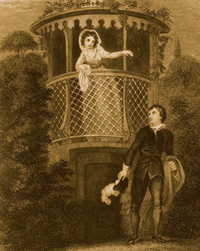
My favorite example of a metaphorical model is a simulator of “Romeo and
Juliet,” intended for high school students studying Shakespeare in English lit
erature classes. Clearly, a simulator cannot possibly replicate Shakespeare’s play,
but it can encourage students to study the play more closely than they otherwise
would. By simulating the waxing and waning of love between Romeo and Juliet,
students become curious about romantic relationships, both in the model and
in the play.4 A metaphorical model is small and can be explained quickly. As we
will see, the “Romeo and Juliet” simulator fits on a single page and involves just aRomeo and Juliet in Brazil 99
Analogue Illustrative Metaphorical
Realistic detail Limited detail Minimal detail
and accurate scaling yet plausible scaling yet transferable insight
High fidelity Simple Low fidelity
Oil
Fishery
Industry
Model Romeo and
Formula 1
Juliet
Figure 6-2. Modeling and realism—a spectrum of model fidelity
handful of concepts, a far cry from the large and detailed model that lies behind
a Formula 1 simulator.
It is important to realize that business models typically lie somewhere in the mid
dle of this spectrum of model fidelity. In the Braskem program, participants were
able to experience this middle range with two more simulators that formed the core
of the program. Closest to the metaphorical model is a simple fishery model (just
10 equations) to explain the syndrome of collapsing fish stocks observed in fisheries
around the world. Further to the left is the oil industry model (containing 100 equa
tions) used to investigate long-term scenarios for oil price and crude oil production
and to shed light on the industry’s volatility. Neither of these models are perfect rep
licas of the industries they represent. Instead they focus on selected dynamics (the
behavior over time of catch and ships in fisheries, and the behavior over time of oil
price, upstream capacity, and demand in the oil industry) and capture just enough
about the feedback structure of the business to explain the dynamics of interest.
Metaphorical Models and Thinking Skills:
Pacific Sardine Fisheries
People rarely think of problems in business and society in terms of dynamics and
behavior over time. Instead they are preoccupied with events and who to blame
when things go wrong. Their ability to express problem situations in dynamic
terms needs to be awakened. In the Braskem course, we began with a vivid exam
ple from the Pacific Coast sardine fishery. The events in the history of the fishery
are described by ecologist Robert Leo Smith.
The Pacific Coast sardine industry had its beginnings back in 1915 and reached its
peak in 1936–1937 when the fishing fleet netted 800,000 tons. It was first in the100 John Morecroft
800
700
Catch (thousands of tons)
600
500
400
300
200
100
0
1916
1924
1932
1940
1948
1956
1964
1972
1980
1988
1996
From Fish Banks, Ltd. Debriefing slides by Dennis L. Meadows et al., in D. L. Meadows, T. Fiddaman, and
D. Shannon (2001), Fish Banks, Ltd. A Micro-computer Assisted Group Simulation That Teaches Principles of
Sustainable Management of Renewable Natural Resources (3rd ed.). Durham, New Hampshire: Laboratory
for Interactive Learning, University of New Hampshire.
Figure 6-3. Puzzling dynamics in fisheries
nation in numbers of pounds of fish caught, and ranked third in the c ommercial
fishing industry, growing $10 million annually. The fish went into canned sar-
dines, fish bait, dog food, oil, and fertilizer. The prosperity of the industry was
supported by overexploitation. The declines in the catch per boat and success per
unit of fishing were compensated for by adding more boats to the fleet. The fishing
industry rejected all forms of regulation. In 1947–1948 the
T ime charts encourage
dynamic thinking, a vital
skill which Barry describes as
Washington-Oregon fishery failed. Then, in 1951, the San
Francisco fleet returned with only eighty tons. The fishery
closed down . . . [Oliver Owen, Natural Resource Conserva-
“the ability to see and deduce tion: An Ecological Approach. New York: MacMillan, 1985.]
behavior patterns rather than
focusing on, and seeking to
predict, events.” Time charts An important step in modeling is to construct time
help modelers to identify charts of selected variables in such problem situations.
feedback structures (or inter Time charts encourage dynamic thinking, a vital skill
dependencies) that explain the which Barry describes as “the ability to see and deduce
observed behavior patterns.
behavior patterns rather than focusing on, and seeking to
predict, events.” Time charts help modelers to identify
feedback structures (or interdependencies) that explain
the observed behavior patterns. For example, Figure 6-3 shows the annual Pacific
sardine catch in thousands of tons over the period 1916 to 1996. The highly
volatile trajectory encapsulates the unfolding catastrophe facing the fishing com
munity in its bid for growth and prosperity. The annual catch grew remarkablyRomeo and Juliet in Brazil 101
change in
Romeo’s love Romeo’s Love
for Juliet for Juliet
Juliet’s Love for Romeo Romeo’s Love for Juliet
Love
in units
of
Time
in months
change in
Juliet’s love Juliet’s Love
for Romeo for Romeo
Figure 6-4. Problem situation: Waxing and waning of love between Romeo and Juliet
between 1920 and 1940, starting around 50 thousand tons and peaking at 700
thousand tons—a fourteen fold increase. Over the next four years to 1944, the
catch fell to 500 thousand tons, stabilized for a few years and then collapsed dra
matically to almost zero in 1952. Since then it has never properly recovered.
Metaphorical Models and Thinking Skills: “Romeo and Juliet”
In the Braskem course, I reinforced dynamic thinking about the rise and fall of fish
eries with dynamic thinking about Romeo and Juliet. Admittedly, this is a fanciful
example in which a conjecture about varying love in a relationship substitutes for
the factual historical time series data found in fisheries; nevertheless, the exercise
enables students to consider the time dimension and scaling of love, despite its
emotional and intangible nature. I began by sketching on a flip chart the axes of the
time chart shown on the right of Figure 6-4. The horizontal axis is time in months
and the vertical axis is love in units of love. Not surprisingly, the vertical axis is
amusing, but it also provokes serious discussion about how, in reality, one might
gauge the strength of an emotional attachment between two people.
I then defined the problem situation as the waxing and waning of love between
Romeo and Juliet and sketched the trajectory of Juliet’s Love for Romeo as a quan
tity that rises and falls cyclically over time. I admit that the fit between this imag
ined trajectory and Shakespeare’s play is somewhat tenuous, but remember this102 John Morecroft
is a metaphorical model whose purpose (if used in literature classes) is to draw
one into the romantic substance of the play rather than to faithfully replicate the
full Shakespearian tragedy.5
Next, I sketched the trajectory of Romeo’s Love for Juliet, which, importantly,
is out-of-phase with the movement of Juliet’s Love for Romeo. The phasing in
Figure 6-4 is simulated and therefore strictly consistent with the model’s struc
ture and assumptions; however, a rough sketch (similar to the kind I drew in
class) need not achieve such consistency in order to show periods of harmony
and conflict within an evolving relationship. Differences in phasing add richness
to dynamic thinking and help to illustrate how events fit within a broader cyclic
pattern. Consider, for example, instances of conflict between Romeo and Juliet
when her rising love, near to the peaks, is reciprocated by a fall in Romeo’s love.
Operational Thinking in “Romeo and Juliet”
Another vital modeling skill is operational thinking, which, as Barry notes, brings
discipline to feedback systems thinking. “It’s here [in operational thinking] that
people must think in terms of units of measure, or dimen
I n operational thinking,
people must think in terms of
units of measure, or dimensions.
sions. Physical conservation laws are rigorously adhered
to in this domain. The distinction between a stock and
Physical conservation laws are flow is emphasized.” In the Braskem course, the fisheries
rigorously adhered to in this example provided an ideal practical situation in which to
domain. The distinction between introduce stocks and flows, and to question why it is so
a stock and flow is emphasized.
difficult for real fishing communities to achieve a sustain
able balance between fish population and fleet size. I omit
the detail of this example here, but invite readers to imag
ine for themselves the aggregate stocks and flows of fish and ships that would
form the basis of a simple-yet-plausible model of fisheries.
“Romeo and Juliet” served to amplify the operational thinking introduced
with fisheries. I began by sketching on a whiteboard just the two stock accumu
lations shown in Figure 6-4: Romeo’s Love for Juliet and Juliet’s Love for Romeo.
We discussed the need for units of love in order to quantify the waxing and
waning of love. We also discussed how these variations in love would be cap
tured in the gradual filling-up or depletion of the two love stocks. Naturally, that
led us to consider the rates of flow that impinge on love: the change in Romeo’s
love for Juliet and the change in Juliet’s love for Romeo. The important distinction
between a stock and a flow is apparent here. Love builds or withers and so a
time-dependent story of love can be told. Changes in love (whether Romeo’s
or Juliet’s) are naturally measured in units of love per month which accumulateRomeo and Juliet in Brazil 103
over time into units of love, thereby ensuring dimensional consistency in the
stock and flow networks. Love springs eternal from the heart, depicted as the
pool from which new love flows or to which spurned love returns.
By now the whiteboard diagram showed two stocks and two flows, as yet
unconnected. To complete the diagram there is a need to recognize the mutual
T
dependence of Romeo and Juliet. They are emotionally his hypothesis came as a big
entwined. Of course there are many ways to express this
surprise to many people
entwinement. But two particular and strikingly simple
connections are all that are needed to produce the cycli and is a powerful example of
cal pattern of love in the time chart. At least that is the a fundamental tenet in system
dynamic hypothesis. If the change in Romeo’s Love for Juliet dynamics—that feedback structure
depends on Juliet’s Love for Romeo, and vice-versa, then an gives rise to dynamic behavior.
endless cycle of waxing and waning love is possible. This
hypothesis came as a big surprise to many people and is
a powerful example of a fundamental tenet in system dynamics—that feedback
structure gives rise to dynamic behavior. In Figure 6-4 there is a closed feedback
loop that weaves its way between and among the stocks and flows of love. There
is no need for any external influence to drive the dynamics of love, not even the
stars and the moon. The tides of love are self-generating.
From this structural diagram, it is a further step to a full-blown simulator.
In my experience, this step is not easy, although it is undoubtedly made more
achievable by the self-imposed rigor of operational thinking and the resulting
diagram like the one shown on the left of Figure 6-4. In the Braskem program, I
asked participants to formulate equations. Initially, they wrote equations for the
two stock and flow networks (using as a template the stock and flow equations
for fish and ships from the simple fisheries model).
All stock and flow equations have exactly the same
syntax because they are accumulations. Like a bathtub, A ll stock and flow equations
have exactly the same
each stock accumulates its inflow (or, in more general syntax because they are
terms, the difference between the inflow and the out
accumulations. Like a bathtub,
flow). Modeling software exploits the syntax similarity by
automatically writing stock accumulation equations. But each stock accumulates its inflow
it is important for beginning modelers to write such equa (or, in more general terms, the
tions for themselves, so they better understand how the difference between the inflow
intuitive yet vital concept of accumulation is expressed and the outflow).
rigorously and mathematically.
After writing equations for the accumulation of love, participants then tackled
the tricky task of formulating equations for causal links between the two lovers.
I allowed participants the freedom to introduce auxiliary concepts in order to
operationally create the links. This exercise, conducted by pairing participants,104 John Morecroft
provoked a lot of thinking and discussion. Participants tried their best to capture
the imagined sensitivity of lovers and argued whether Romeo and Juliet respond
to being loved in exactly the same way or somehow mirror each other’s affec
tions. The model was small enough that everyone managed to formulate a full-
set of equations and run simulations. The result was a wide variety of time charts.
Some charts showed escalating growth of love while others showed a collapse of
love to a permanent state of cold lovelessness (zero units of love).
In the limited time available, nobody was able to reproduce a cyclical pattern
of love; nevertheless, the exercise of developing the model and equations pro
voked much fruitful thought about the relationship between Romeo and Juliet,
T he discipline of operational
just as a metaphorical model should. With a bit more time
after the course was completed, it was possible to formu
thinking about Romeo and
late equations that generate cyclicality. They are listed in
Juliet takes one deeply into the Appendix 1 and are not especially difficult to understand
problem situation and, with patience, (see also Appendix 2 for an equation description).6 But
can yield an insightful simulator. the difficulty of writing equations that mean what you
The same applies to business and intend (and of being absolutely clear about what you
really mean) underscores an enduring challenge of good
industry models, and that was the
modeling. It is not easy to build full-blown simulators
message I wished to convey. (even small ones), and there is always room to improve
formulation skills; however, the discipline of operational
thinking about Romeo and Juliet takes one deeply into the problem situation
and, with patience, can yield an insightful simulator. The same applies to busi
ness and industry models, and that was the message I wished to convey.
Structure and dynamic behavior in “Romeo and Juliet”
A causal loop diagram of the relationship between Romeo and Juliet is shown
in Figure 6-5. It was a good opportunity to practice basic diagramming rules
in preparation for the multi-loop oil producers’ model. Essentially, Romeo and
Juliet’s love for each other is mutually dependent, and it is this interdependence
that forms the closed feedback loop of their relationship. Our picture shows not
only love but also changes in love.
As Romeo’s Love for Juliet grows, it causes the change in Juliet’s love for Romeo
to increase (which is depicted as a positive link). Such increments of love make
Juliet’s Love for Romeo stronger, another positive link. In other words, her love
thrives on affection. Romeo is different and he spurns affection. So, as Juliet’s
Love for Romeo grows, it causes the change in Romeo’s love for Juliet to decrease,
(which is depicted as a negative link). Such deductions from (the stock of) love
make Romeo’s Love for Juliet weaker, a kind of positive link.7 In other words, his
love withers with affection and is nurtured by disdain.Romeo and Juliet in Brazil 105
4
Balancing loop Juliet’s Love for Romeo Romeo’s Love for Juliet
+ Romeo’s Love
for Juliet
0
Tides of +
change in Romeo’s change in Juliet’s
love for Juliet love for Romeo -4
0 12 24 36 48
B Months
–
2
change in Juliet’s Love for Romeo
Juliet’s Love
for Romeo +
0
change in Romeo’s Love for Juliet
-2
0 12 24 36 48
Months
Figure 6-5. Causal loop diagram and simulations of Romeo and Juliet
The four links make a closed loop, which is named “Tides of Love” and is
shown as a balancing loop B. This polarity says that the loop counteracts spon
taneous change. For example, if Romeo’s Love for Juliet were to increase (due to
an imagined exogenous event like the arrival of spring), then the strictures of
their closed loop relationship would bring about a counteracting decrease in his
love. In this thought experiment, Romeo’s springtime ardor induces an increase
in Juliet’s Love for Romeo, which accumulates. Her greater love in turn induces
a decrease in Romeo’s Love for Juliet, thereby closing the loop and counteract
ing the original increase. Of course, if Romeo’s love were to thrive on affection
rather than to wither, his relationship with Juliet would be transformed into a
reinforcing loop and their love would grow without bounds.
Behavior Analysis in “Romeo and Juliet”
(“Understanding Oscillations”)
Simulations of the “Romeo and Juliet” model are shown on the right of Figure
6-5. It turns out that the two are locked in an endless cycle of waxing and waning
love, as originally postulated. But the simulations help to explain this puzzling106
over time (which, as mentioned, surprises many people and alerts them to the
subtlety of dynamics, even in apparently simple systems).8 My interpretation
mimics the style of behavior analysis in “Understanding Oscillations” and takes
then, the oscillations of interest arose from a simple inventory-workforce model
of a factory. But remarkably, interdependencies in a factory
Interdependencies in a factory
bear an uncanny resemblance
to the closed-loop relationship
bear an uncanny resemblance to the closed-loop relation-
ship between Romeo and Juliet, as further illustrated in
between Romeo and Juliet.
two time charts (Figure 6-5), the top chart showing stocks
-
tion, Juliet’s Love for Romeo is two units of love while Romeo’s Love for Juliet is one
the change in Juliet’s Love for Romeo has fallen to zero, meaning that there is no
longer cause for her love to change. She is in a period of contented and stable
love. But this state does not and cannot last. By month 1, Romeo’s love has fallen
to zero and the rate of change of his love is at a minimum of minus one units of
love per month. He does not share Juliet’s stable contentment and his love for
Juliet continues to fall, reaching a low of slightly more than minus two units of
period of three months. Her love for Romeo gradually recedes and reaches zero
by month 5. By now she is quite upset with Romeo and the rate of change of her
love reaches a low of minus one units of love per month. Inevitably, this further
deterioration in their relationship causes her love to fall still further, becoming
negative in value and reaching a minimum of slightly more than minus two by
-
tion and his disdain for Juliet begins to lessen, so that,
T he metaphorical model,
“Romeo and Juliet,” when
developed and completed,
by month 9, his love returns to zero and is growing at
its fastest rate just as Juliet’s love reaches its nadir.
presents a good example of Romeo’s
closed-loop thinking , one of Love for Juliet continues to rise for four months, reach-
Barry’s eight types of systems ing a peak of slightly more than two units by month 13.
thinking.
in Juliet. Her love climbs from its negative depths to a
calm neutrality of zero by month 13. But this seeming
neutrality does not last as her love continues to grow, spurred on by Romeo’sRomeo and Juliet in Brazil 107
themselves back in exactly the same romantic state they were at the start of the
simulation. Juliet’s Love for Romeo is at two units of love and rising, while Romeo’s
Love for Juliet is at one unit and falling. The stage is set for another identical cycle
of love.9 The metaphorical model, “Romeo and Juliet,” when developed and
completed, presents a good example of closed-loop thinking, one of Barry’s
eight types of systems thinking.
Dynamic and Operational Thinking about Oil Production
Fisheries and Shakespeare occupied the first morning of the program and paved
the way for the Oil Producers’ Microworld in the afternoon. The Microworld is
a gaming simulator that captures the dynamic interplay of three groups of oil
producers whose combined production determines the world supply of crude
oil; however, their reasons for investing and producing are very different.
Commercially motivated, independent producers are represented by companies
like Shell, Exxon Mobil, and BP Amoco. Politically motivated OPEC producers
include the swing producer (Saudi Arabia), and opportunists are represented
by developing countries such as Nigeria. The contrast of world views among
these diverse stakeholders was well-suited to the international theme of the
Braskem program. These world views are bound together in multiple feedback
loops, which are coded as the Microworld’s diverse alternative futures for the oil
industry.
Participants were organized into competing teams who played the role of
independents. Teams make yearly upstream capacity investment decisions over
twenty-five simulated years, with an objective to make as much money as possible.
Success depends on developing investment strategies and policies suited to the
selected industry scenario. Scenarios, in turn, reflect the influence on the industry
of the other producer groups and their strategic goals, as well as global economic
pressures on demand. In the Braskem course, we used a topical scenario entitled
“Asian Boom and Bust.” The team with the highest cumulative net income in 2020
was to be the winner of the competition.
An important objective of the exercise was for participants to look inside the
Microworld to understand how the industry is modeled (rather than treating the
simulator as a mysterious black box). Therefore the pre-game briefing involved
dynamic and operational thinking about the industry.
We began with the turbulent history of oil price, as shown in Figure 6-6,
spanning a period of 130 years from 1869 to 2004. There are striking contrasts
between periods of price stability, mild price fluctuations, dramatic price surges,
and equally dramatic collapses. Between 1869 and 1880, there was extreme price108 John Morecroft
volatility corresponding to the early pioneering days of the oil industry in the
Pennsylvania oil regions of the United States. Following the early extreme price
fluctuations was an interval of mildly cyclical oil price in the decades between
1889 and 1929. This marked reduction of volatility was brought about by John D.
Rockefeller, founder of Standard Oil, who set about controlling supply through
ownership of refining and distribution.
In the pre-war and post-war era from 1930 to 1970, the reformed oil indus
try structure remained in place—almost unchallenged—even as the indus
try expanded internationally on the back of colossal reserves in the Arabian
Peninsula. Throughout this era, spanning four decades, supply and demand were
in almost perfect balance—an astonishing achievement when one considers the
complexity of the industry.
But new forces were at work, ushering in a new era of oil supply politics. As the
locus of production moved to the Middle East, the global political power of the
region was awakened, feeding on the appetite of western industrial countries for
Arabian oil to sustain their energy-intensive economies and lifestyles. Control
over Middle Eastern oil was seized by newly formed OPEC (the Organization of
Petroleum Exporting Countries). In 1974, and again in 1978, OPEC exercised
its power by decreasing production and forcing up the price of oil. As Figure 6-6
shows, the price doubled and continued to rise to a peak of almost 70 dollars
per barrel by 1979—a peak not seen since the early days of the Pennsylvania oil
boom in the nineteenth century. So, in the 1970s, after two decades of managed
calm and predictability, chaos returned to global oil markets.
After 1978, oil price fell sharply to only 20 dollars per barrel in the mid-1980s.
For more than twenty years there were no further upheavals to match the dra
matic variations of the 1970s. As the turn of the century approached, oil price
was stable and low at 15 dollars per barrel. In fact, many observers at the time
believed it would stay low for the foreseeable future. But the industry proved
them wrong. Instability reminiscent of the 1920s and early 1930s, triggered by
regional wars, power struggles within OPEC, fears of shortage, and extremes of
weather started to affect oil production. Price began to rise again in 2001, reach
ing more than 30 dollars per barrel by 2004. This upward trend continued to 60
dollars per barrel in 2006, and, as we all know, to more than 100 dollars per bar
rel in 2008 (expressed in constant 2006 dollars).
Clearly, there is a lot to explain in the detail of this fascinating chart covering
such a long span of time. It is troublesome that the price of such a vital commodity
as oil can vary so much. The implications are enormous for industrialized societies,
OPEC states, developing countries, oil companies, chemical companies, and con
sumers. Western economies are painfully affected when the price of gasoline rises
sharply. It is even more painful in OPEC economies when the national budgetRomeo and Juliet in Brazil 109
U.S. FIRST PURCHASE (Wellhead)
1869–August 2007
WTRG Economics ©1998-2007
World Price Avg U.S. $21.05 www.wtrg.com
(479) 293-4081
Avg World $21.66 Median U.S. & World $16.71
Figure 6-6. Historic crude oil price, 2006 dollars
shrinks in half or less during an oil price collapse. Yet, among the wild extremes of
price over 150 years, prolonged periods of stability have been experienced in the
1930s, 1950s, and 1960s. Perhaps such stability is even more remarkable than vola
tility. Operational thinking about the oil industry can help to explain these episodes.
Following is a sample of the operating structure from the Oil Producers’ Microworld
that explains industry stability (see Morecroft 2007, Chapter 8 for more details).
The same material was presented to Braskem and gives a feel for the amount of
model detail revealed to participants in preparation for the simulation competition.
Oil production capacity expansion by the independent producers
The independents expand production capacity when they judge it is profitable to
do so, as shown in Figure 6-7. Note that, in the Microworld, this judgment is left
entirely up to the discretion of players. The circular symbol is the capacity expan
sion policy, commonly called capex, that controls the flow of new capacity into the
stock of capacity controlled by independents. Figure 6-7 shows the main informa
tion sources that are available to calculate the profitability of investment projects.
Independents estimate the development costs of new fields and the expected
future oil price over the lifetime of the field. Knowing future cost, projected oil110
Tax
Hurdle change in
independent Independent
rate Producers’
producers’
capacity Capacity
Independents’
development
cost
Expected
future oil price
Market Capex
oil price optimism
Figure 6-7. Independents’ capacity expansion a commercial worldview
acceptable projects. In reality, each project undergoes a thorough and detailed
capacity, the bigger the independents become and the more projects are in their
portfolio of investment opportunities.
Executive control of recommended expansion is exercised through capex
investment optimism that captures collective investment bias among top man-
agement teams responsible for independents’ investment.
W e are not concerned with
the detail of individual
oil field projects; rather, we are
Optimism can be viewed on a scale from low to high. High
optimism means that oil company executives (game play-
ers) are bullish about the investment climate and approve
seeing the commercial pressures
for oil production capacity would suggest. Low optimism means executives are cau-
expansion in the aggregate.
tious and approve less expansion than recommended. It
is important to appreciate the distance from which we are
viewing investment appraisal and approval. We are not
the commercial pressures for oil production capacity expansion in the aggregate.Romeo and Juliet in Brazil 111
Strictly speaking, there is a two-stage stock accumulation process for upstream
Output of the “swing producer” of oil
For many years the swing producer in the oil industry has been Saudi Arabia.
to defend OPEC’s intended price, known in the industry as the “marker price.”
A producer taking on this role must have both the physical and economic capac-
ity to increase or decrease production quickly, by up to 3 million barrels per day
for example, to an unusually mild winter or hot summer) and/or to compensate
important assumption that the swing producer always has adequate capacity to
meet any call for oil it receives.
Production responds to pressure both from production quotas and from oil
Ministers change production in order to meet the swing producer’s allocated
quota. But they also take corrective action whenever the market oil price devi-
ates from OPEC’s intended price. When the price is too low, Saudi production
is reduced below quota thereby undersupplying the market and pushing up
the market price. Conversely, when the price is too high, Saudi production is
Market Swing Swing
oil price producer producer
change in production
production
Intended
price
Swing producer’s
allocated quota
Figure 6-8. Swing producer’s policy a political worldview112 John Morecroft
increased above quota to oversupply the market and reduce the oil price to the
level OPEC is trying to defend. Such ability and willingness to rapidly adjust
production is characteristic of any swing producer.
Sometimes the swing producer floods the market with oil in order to drive
down the price and gain market share. This punitive mode of production is part
of the full model, but is not included in the sample of structure presented here.
Feedback loops in global oil production
Figure 6-9 shows the main feedback loops formed by the independents and by
the swing producer. These loops play an important role in balancing supply and
demand in the global oil industry. Balancing loop B1 is the industry’s main com
mercial supply loop. A production shortfall stimulates a rise in Market Oil Price
and an increase in the price-to-cost ratio, which makes upstream investment more
B ecause it takes many years
attractive for commercial oil companies. As a result, there
is an increase in capacity approval and capacity in construc-
to develop new capacity,
tion, which eventually leads to expansion of Independents’
this feedback loop alone does Operating Capacity and actual independents’ production.
not ensure that supply always Extra production corrects the production shortfall and
matches demand. Market forces completes loop B1. Because it takes many years to develop
alone cannot stabilize oil price.
new capacity, this feedback loop alone does not ensure
that supply always matches demand. Market forces alone
cannot stabilize oil price.
In fact, price stability comes from the swing producer. OPEC production
in the lower half of the figure is the sum of Swing Producer Production and the
Opportunists’ Production. When the member states are in harmony, they pro
duce according to negotiated quota; however, the swing producer will depart
from negotiated quota when there is a difference between the intended marker
price and Market Oil Price. This connection to Market Oil Price closes a balanc
D espite OPEC’s reputation
ing feedback loop B2 that passes back through production
shortfall and OPEC production before reconnecting with
for aggressive price hikes,
Swing Producer Production. This fast-acting balancing loop
the swing producer is in fact a is capable of creating prolonged periods of price stabil
benign and calming influence in ity as seen in the 1960s. When market price falls below
the global oil market, boosting or the intended marker price due to a temporary supply glut,
curtailing production in order to the swing producer quickly cuts production below nego
tiated quota to bring price back in line with the target or
maintain stable prices.
marker. The loop acts quickly because the swing producer
is willing to make capacity idle—a process that takes only
a month or two. Similarly, when market price rises above the intended marker
price due to a temporary demand surge, the swing producer quickly re-activatesRomeo and Juliet in Brazil 113
+
Capacity in
Construction
+ capacity
approval
B1 +
+
– Independents’
capex hurdle commercial Operating Capacity
optimism rate supply
price-to-cost
ratio
+ + development and
operating cost per +
intended
Market barrel independents’
marker price
Oil Price production
+
– production
shortfall –
+ price
gap B2 demand + –
for oil
OPEC
price OPEC production
control
+ + Opportunists’
Production
Swing Producer
– Production +
+ swing producer opportunists’
negotiated negotiated quota
quota
Figure 6-9. Feedback loops involving independents and the swing producer
idle capacity to increase supply and bring price down. Despite OPEC’s reputa
tion for aggressive price hikes, the swing producer is, in fact, a benign and calm
ing influence in the global oil market, boosting or curtailing production in order
to maintain stable prices.
Similar discussion of the remaining operating policies, stock accumulations,
and feedback loops in the oil producers’ model completed the pre-game brief
ing given to the participants. At that point the chosen teams were ready to play
the Microworld. Like a bevy of earnest Juliets, they pitted their wits against
fickle OPEC and global consumers under a scenario of Asian boom and bust.
The sought-after prize was evening dinner for the winning team at an elegant114 John Morecroft
restaurant in the Guarajuba resort. The contest was fierce but nevertheless enjoy
able. Using an involved and interactive style to systems thinking created not only
a game situation but a fundamentally important approach to management situ
ations and problems.
In this paper, I have reviewed the models and simulators used in a two-day mod
ule on system dynamics for Braskem managers. Models are intended to help us
make sense of our complex and interconnected world, to foresee (amid complex
ity) the consequences of strategic change, and to avoid pitfalls. Doing so requires
much more than technical skills in the use of modeling software or a flair for
P eople need conceptual
gaming simulations. People also need conceptual skills
to appreciate interdependencies in business and society
skills to appreciate
(often hidden from everyday view) and how they lead to
interdependencies in business puzzling dynamics in the events we experience and in the
and society (often hidden from very problems we are trying to solve.
everyday view) and how they lead In the Braskem program, we used a spectrum of mod
to puzzling dynamics in the events
els, from “Romeo and Juliet” to fisheries and global oil, to
illustrate some of the conceptual skills of the modeler and
we experience and in the very
feedback systems thinker. These skills are important for
problems we are trying to solve. general managers as well. Time charts encourage dynamic
thinking to find, among the flux of events, patterns of
behavior over time (whether it be volatile oil price, the rise and fall of fish catch,
fluctuating love, or the expected outcome of a new strategy). From such pat
terns of behavior there is the imaginative and creative step of operational think
ing to find, among interlocking decisions and actions, the stock accumulations
and feedback loops from which dynamics arise. In “Romeo and Juliet,” there is
just one feedback loop which, to the surprise of many, can generate an endless
cycle of waxing and waning love. In global oil, the interplay of many feedback
S
loops connecting commercial producers, consumers, and
imulation reliably computes
OPEC creates both turmoil and stability in the oil indus
these outcomes, but it
try and in oil prices. Simulation reliably computes these
is the discipline of feedback outcomes, but it is the discipline of feedback systems
systems thinking that makes clear thinking that makes clear the structure that lies behind
the structure that lies behind simulated behavior. The mysteries of the simulator, and
simulated behavior.
its chosen slice of reality, are revealed so it is no longer a
black box.
It was the desire to illuminate the thinking behind the Oil Producers’ Microworld
that led to the content of the Braskem course with its blend of large and smallRomeo and Juliet in Brazil 115
models. And so the smallest model, “Romeo and Juliet,” became a metaphorical
model to awaken feedback systems thinking among one group of managers in a
single region of vast and beautiful Brazil. It was part of Barry’s quest to bring sys
tems thinking to the world.
References
Mass NJ and Senge PM 1975. Understanding Oscillations in Simple Systems,
MIT System Dynamics Group Working Paper, D-2045-2 (available from the
System Dynamics Society on a DVD containing the complete D-memo series of
the MIT System Dynamics Group).
Morecroft JDW 2007. Strategic Modeling and Business Dynamics, Wiley, Chichester.
Owen, Oliver. Natural Resource Conservation: An Ecological Approach. New York,
N.Y.: MacMillan, 1985.
Radzicki MJ 1993. “Dyadic Processes, Tempestuous Relationships, and System
Dynamics,” System Dynamics Review, 9 (1), 79–94.
Richmond BM 1985. A User’s Guide to STELLA, High Performance Systems Pub-
lications, New Hampshire. (High Performance Systems subsequently became
isee systems.)
Richmond BM 1977. Senior Executives System Dynamics Workshop Session II:
Inventory-Workforce Model, MIT System Dynamics Group Working Paper,
D-2661 (available from the System Dynamics Society on a DVD containing
the complete D-memo series of the MIT System Dynamics Group).
Strogatz SH 1988. Love Affairs and Differential Equations, Mathematics Magazine,
61 (1), 35. 10.
Notes
1. Oscillations continued to fascinate Barry and became an important part of his
repertoire for communicating systems thinking. Already, in 1977, he was conducting
workshops in the MIT Senior Executives program using the inventory-workforce
model to introduce system dynamics concepts. He begins his workshop notes
(Richmond 1977) by stating that the purpose of the session is:
To illustrate three major system dynamics concepts:
(1) Internal structure has inherent behavioral tendencies. Structure gives
rise to behavior. External factors precipitate response.
(2) Transferability of structure.
(3) Difficulty of performing an intuitive policy analysis even with a formal
(explicit) model (and a simple one at that!).
The notes include a structural diagram and equation listing for the inventory-work-
force model and simulations (hand-drawn trajectories to join-up character plots)
that show how different disturbances in demand (step-increase, ramp, and pulse) all
precipitate cyclical variations in inventory, production, and workforce.116 John Morecroft
Also, the first user guide to STELLA includes a section devoted to the oscillatory
dynamics of a predator-prey model, as the following excerpt shows:
Now here is a tough question for you. Why does this system oscillate? Think
about it for a minute. You might want to review the model structure, analyze a few
graphs and change some parameters before drawing any conclusions. The model
you just constructed is not only a simple model of predator-prey dynamics. It has
the generic structure of a pure oscillator. (The structure governing the motion
of a pendulum, an oscillator we are all familiar with, is almost identical to your
two-stock model.) The key to the oscillatory behavior is in the way the two stocks
are linked. When prey reaches a peak, the predator population is at its most rapid
rate of expansion. Similarly, when predators are at the low ebb of their cycle, prey
population is at its most rapid rate of expansion.”
2. The paper begins with a single stock model of the rabbit population in a field to rigor-
ously demonstrate (by simulation) that a model containing a single stock accumula-
tion cannot possibly generate overshoot or cyclical dynamics. A model requires at
least two stocks to generate oscillations. The authors develop an inventory-workforce
model containing two stocks and only four active equations (eleven equations includ-
ing constants and initial values) to rigorously demonstrate the origin of undamped
oscillations in a second-order system. Realistic extensions to this tiny model are then
used to explain both expanding and damped oscillations. These structural variations
on the base model are similar to the structural variations that Mike Radzicki adds to
his Romeo and Juliet model to investigate dynamics and romantic styles.
3. I would also like to acknowledge Isabella Schiavinato and Soraia Cardoso for their
enthusiastic and professional support during the Braskem course. Thanks, too, to Ana
Cristina Dias, Coordinator HR at Braskem, who kindly secured permission for details
of the course to be included in this paper.
4. The Romeo and Juliet simulator comes from a paper by WPI’s Mike Radzicki,
published in the System Dynamics Review which, in turn, was built on an article by
Harvard’s Steven Strogatz in Mathematics Magazine (see the annotated bibliography at
http://iseesystems.com/tracing for more details of both papers). The model’s original
purpose was to engage the interest of Steven Strogatz’s undergraduate students who
were studying differential equations. By translating the differential equation model
into stocks, flows, and feedback loops Mike Radzicki found it to be a useful model
for engaging the interest of students studying system dynamics. English literature
students may not understand differential equations, but they can appreciate romantic
relationships expressed in the visual language of stocks, flows, and feedback loops.
5. In the model of Romeo and Juliet, it is not their families that keep them apart; instead,
it is Romeo’s fickleness. Nevertheless, the model does touch on themes such as love,
time, fate, and chance that students of Shakespeare are often asked to consider. For
example, the Wikipedia entry about Romeo and Juliet mentions that “time plays an
important role in the language and plot of the play . . . For instance, when Romeo at-
tempts to swear his Love to Juliet by the moon, Juliet tells him not to, as it is known to
be inconstant over time, and she does not desire this of him.”
6. The appendices for this chapter as well as for the rest of the book are available at
http://iseesystems.com/tracing.
7. The assignment of polarity to this link is tricky because the link corresponds to a bi-flow
in a stock accumulation process. Here one could justify a positive link on the grounds of
a double negative effect—deductions from love make Romeo’s love for Juliet weaker.Romeo and Juliet in Brazil 117 8. Readers can recreate the simulated trajectories and study them more closely by run- ning the Romeo and Juliet simulator that accompanies this chapter and can be found at http://iseesystems.com/tracing. 9. By carefully analyzing the shape of the trajectories for change of love and the areas they enclose, it is possible to prove they are symmetrical around their peaks and, therefore, that a perfect undamped harmonic oscillation is unfolding. Such graphical proof is beyond the scope of this paper, but a similar proof for the inventory-workforce model can be found in the original article on “Understanding Oscillations.”
118   John Morecroft

        The Loops of Feedback
         A verse inspired by 30+ years of system dynamics and a famous song, called
        “The Streets of London,” by British folk singer Ralph McTell. Incidentally, I saw
         him perform the song live in 2006, at a festival in North Cornwall marking the
         centenary of the birth of English Poet Laureate John Betjeman.

        Have you seen the asset stocks in the multi-looped beer game?
        Amplifying orders when consumers drink more beer.
        The factory’s working overtime and still the stocks are in decline.
        Feast then turns to famine, but the reason is unclear.

         Refrain (to be sung after each verse):
         So how can you tell me that life’s optimal.
         Don’t say we’re rational all the time.
         Let me take you by the hand.
         I’ll lead you through the loops of feedback.
         I’ll show you something that will make you change your mind.

        In the Fish Banks model, at the fish rate formulations,
        There are non-linear functions confounding fishermen’s lives.
        Their ships return empty when once there was plenty.
        The sudden collapsed fishery is yesterday’s surprise.

         Have you glimpsed intangibles within the airline simulator
         Determining the destiny of People Express?
         Declining motivation and service degradation
         Feed back to undermine the firm’s growth and success.

        Have you seen the coiled-up slinky’s fascinating oscillations
        Showing that in structure dynamic patterns lie?
        There’s no need for forcing factors only nature’s spring-mass strictures
        Plus the covert force of gravity’s steady tie.

         Refrain.

                                                                                  (cont.)
Romeo and Juliet in Brazil 119
Have you heard of misperceptions, turning into paradoxes
In the way that systems behave over time?
Information overrun and localised rules of thumb
Cause not only cycles but stagnation and decline.
The original “The Streets of London” carried a positive message that life is
better than we think, especially when compared with homeless people who
roam the streets of London and face real hardship. I wanted to end this song on
a positive note too, so I added this extra verse:
In all problem situations, there are hidden feedback loops,
Shaping how events unfold within our times.
Despite complex society there’s no need for anxiety.
Just design better policies and we’ll all lead better lives.
Optional Ending Refrain (slightly modified):
So even though life is not optimal.
And we’re not truly rational in our minds.
Let me take you by the hand.
I’ll lead you through the loops of feedback.
Together we’ll find something that will lead to better times.
—Based on “The Streets of London”
John Morecroft, March 2007
extra slinky verse for Barry, June 2008
Academic note: The song and its refrain question the views of policy advisers
who believe that the rigorous rationality of free markets prevails and will solve
the problems faced by society. Instead, we need “loops of feedback” to make
sense of our complex and interdependent world.You can also read